|
Size: 14591
Comment:
|
Size: 14667
Comment:
|
| Deletions are marked like this. | Additions are marked like this. |
| Line 104: | Line 104: |
| * '''nAvg''': For averaged files, number of trials that were used to compute this file. | * '''Leff''': Effective number of averages. For averaged files, number of trials that were used to compute this file. |
| Line 111: | Line 111: |
| * '''select''': Not used anymore. | * '''select''': Indicates if the event group should be displayed in the viewer. |
Tutorial 15: Import epochs
Authors: Francois Tadel, Elizabeth Bock, Sylvain Baillet
We can consider that our datasets are clean from any major artifact. We will now proceed to the analysis of the brain signals we recorded in response to the auditory stimulation. There are two major types of processing workflows for MEG/EEG, depending on whether we are dealing with an event-related paradigm or a steady-state/resting-state study.
This tutorial will only focus on the event-related case: series of stimuli are sent to the subject and we have the corresponding triggers marked in the recordings. We will base our analysis on these triggers, import short epochs around each of them and average them. You will find in the advanced tutorials a scenario of MEG resting-state analysis.
Contents
Import in database
Until now, we've only been looking at data that was read from continuous files. The raw file viewer provides rapid access to the recordings, but many operations can only be applied to short segments of recordings that have been imported in the database. We will refer to these as "epochs" or "trials".
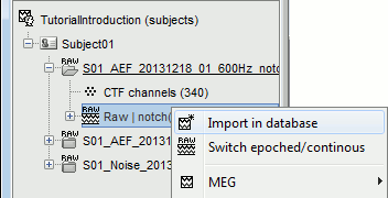
Right-click on Run#01 > Import in database.
Set the import options as described below:
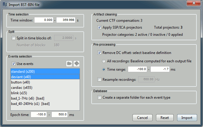
Time window: Time range of interest. We are interested by all the stimulations, so do not change this parameter. The default values always represent the entire file.
Split: Useful to import continuous recordings without events, to import successive chunks of the same duration. We do not need this here.
Events selection: Check the "Use events" option, and select both "standard" and "deviant".
The number between parenthesis represents the number of occurrences of each event in the selected time window (changes if you modify the time definition at the top of the window)Epoch time: Time segment that is extracted around each event marker. Set it to [-100,+500]ms.
Apply SSP/ICA projectors: Use the active projectors calculated during the previous pre-processing steps. Always check the summary of the projectors that are selected.
Here there are 2 categories ("cardiac" and "blink") with a total of 3 projectors selected (one in "cardiac" and two in "blink", the blink and the saccade). Keep this option selected.Remove DC Offset: Check this option, select Time range: [-100, -1.7]ms. For each epoch, it will:
- Compute the average of each channel over the baseline (pre-stimulus interval: [-100,-1.7]ms)
- Subtract it from the channel at every time instant (full epoch interval: [-100,+500]ms).
- This option removes the baseline value of each sensor. In MEG, the sensors record variations around a somewhat arbitrary level, therefore this operation is always needed, unless it was already applied during one of the pre-processing steps.
- Note that a high-pass filter with a very low frequency (for instance 0.3Hz) can efficiently replace this DC correction. If a high-pass filter has already been applied to the recordings, you may want to unselect this option.
Resample recordings: Keep this unchecked.
Create a separate folder for each epoch type: Do not check this option.
- If selected: a new folder is created for each event type ("standard" and "deviant")
- If not selected: all the epochs are saved in a new folder, the same one for all the events, that has the same name as the initial raw file. This is what we want because we have two acquisition runs with different channel files (different head positions and different SSP projectors) to import for the same subject. If we select this option, the "standard" epochs of both runs would be imported in the same folder and would end up sharing the same channel file, which is not correct.
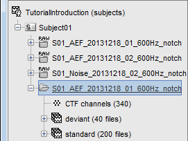
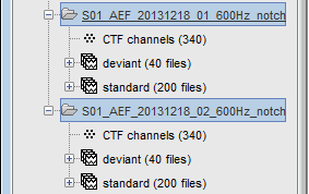
One new folder appears in Subject01. It contains a channel file and two trial groups.
- The channel file is copied from the continuous file.
- To expand a group of trials and show all the files: double-click on it or click on the "+" next to it.
- The SSP projectors calculated in the previous tutorial were applied on the fly while reading from the continuous file. These epochs are clean from eye blinks and power line contamination.
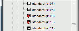
Note that the trials that are overlapping with a BAD segment are tagged as bad in the database explorer (marked with a red dot). All the bad trials are going to be ignored in the rest of the analysis, because they are ignored by the Process1 and Process2 tabs (see next tutorial).
Review the individual trials
After reviewing the continuous file with the "columns" view (channels one below the other) it can be useful to also review the imported trials with the "butterfly" view (all the channels superimposed).
- Double-click on the first trial for the "deviant" condition.
Switch to the "butterfly" display mode: in the Record tab, click on the first button in the toolbar.
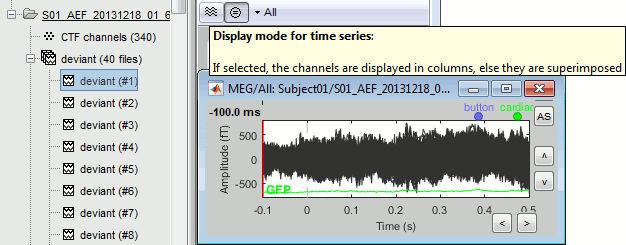
Right-click on the figure > Navigator > Next data file, or use the keyboard shortcut F3.
This way you can quickly review all the trials to make sure that there is no obvious problem.
Mac users: The keys "Fx" are obtained by holding the "Fn" key simultaneously.
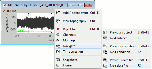
To manually tag a trial as bad, you have three options:
Right-click on the trial file in the database > Reject trial.
Right-click on the figure > Reject trial.
Use the keyboard shortcut Ctrl+B.
To set all the trials back as good in a group: right-click on the trials group > Accept bad trials.
Raster plot
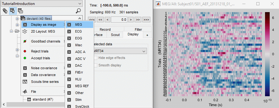
You can also get an overview of the values of one specific sensor over all the trials at once.
Right-click on the group of trials "deviant" > Display as image > MEG.
- You can change the selected sensor with drop-down menu in the Display tab, or use the up/down arrows on your keyboard after clicking on the figure.
The bad trials are already marked, but if they were not this view could help you identify them easily.
Run #02
Repeat the same operations for the second dataset:
Right-click on Run#02 > Import in database.
Import events "standard" and "deviant" with the same options.
Epoch length
We imported epochs of 600ms (100ms baseline + 500ms post-stimulus) but did not justify this choice.
The length of the epochs you import should be chosen very carefully. If you realize later your epochs are too short or too long, you would have to start over your analysis from this point.
The epoch length to consider depends on:
The experimental design
- The minimum duration between two stimuli defines the maximum length you can consider analyzing after the stimulus. You should design your experiment so that it always includes the entire evoked response, plus an additional segment that you can use as a baseline for the following epoch.
- In this study, the inter-stimulus interval (ISI) is random between 0.7s and 1.7s. The minimum ISI (700ms) is long enough to include the entire auditory evoked response, but not the button press that follows a deviant tone. In some cases (late subject response and short ISI), the following stimulation occurs while the brain is still processing the button press. The baseline of some epochs may contain motor and somatosensory components.
- For data processing, it is always better to have longer ISI, but it also means increasing the duration of the experiment or decreasing the number of repetitions, which leads to other problems. The trade-off between data quality and recording time in this experiment is acceptable, very few trials are actually contaminated by the motor response to the previous trial. We will ignore this problem in the following tutorials, but you could decide to reject these few trials in your own analysis.
Here we consider only a short baseline (100ms) to avoid including too much motor activity.
We will only study the auditory response, therefore 500ms post-stimulus is enough.
The processing pipeline
You may have to artificially extend the epochs of interest for technical reasons. Most filters cause edge effects, ie. unreliable segments of data at the beginning and the end of the signal. When applied on short epochs, they might destroy all the data of interest.
For avoiding this, you can add a few hundred milliseconds before and after your epoch of interest. It doesn't matter if it overlaps with the previous or the next epoch. After running the operations that required longer signals, you can cut your epochs back to the desired epoch length. Examples:
Time-frequency (Morlet wavelets):
When estimating the power at frequency f Hz, you get incorrect values for at least one period (T=1/f) at the beginning and the end of the signal. For example, at 2Hz you need to discard the first and last 500ms of your time-frequency maps (1/2Hz=0.5s).Low-pass filtering:
With any filtering operation there will always be a transient effect at the beginning of the filtered data. After filtering, you need to discard the time windows corresponding to these effects. Their duration depends on the order of the filter: this is documented in the tutorial Power spectrum and frequency filters.Hilbert transform:
Same considerations as for the low-pass filter. This process starts by filtering the signals in various frequency bands, using the same function as the band-pass and low-pass filters.Normalizations:
The normalization procedures that use a baseline from the same epoch (Z-score, ERS/ERD, baseline correction) usually work better with longer baselines. The longer the clean baseline, the better the estimation of the average and standard deviation over this baseline. If your baseline is too short, the quality of your normalization will be low.
If you normalize time-frequency maps or filtered source averages, you have to additionally exclude the edge effects from the baseline, and consider an even longer baseline.
In this tutorial, we decided to work with very short epochs (600ms only) so that all the analysis would run on most computers, including personal laptops. For any type of frequency analysis on the recordings, this will be too short. When processing your own recordings, you should increase the size of the epochs beyond the segment that you are actually planning to study.
On the hard drive
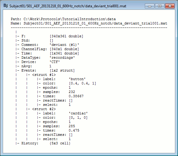
Right-click on any imported epoch > File > View file contents:
Structure of the imported epochs: data_*.mat
F: [Nchannels x Ntime] recordings time series, in Volts.
Std: [Nchannels x Ntime] Standard deviation or standard error, when available (see next tutorial).
Comment: String displayed in the database explorer to represent this file.
ChannelFlag: [Nchannels x 1] One value per channel, 1 means good, -1 means bad.
Time: [1 x Ntime] Time values for each sample recorded in F, in seconds.
DataType: Type of information saved in the F matrix.
Device: Name of the acquisition system used to record this file.
Leff: Effective number of averages. For averaged files, number of trials that were used to compute this file.
Events: Time markers available in the file (stimulus triggers or other events)
label: Name of the event group.
color: [r,g,b] Color used to represent the event group, in Matlab format.
epochs: [1 x Nevt] Only ones for imported epochs.
times: [1 x Nevt] Time in seconds of each marker in this group (times = samples / sfreq).
For extended events: [2 x Nevt], first row = start, second row = end.reactTimes: Not used anymore.
select: Indicates if the event group should be displayed in the viewer.
channels: {1 x Nevt} Cell array of cell-arrays of strings. Each event occurrence can be associated with one or more channels, by setting .channels{iEvt} to a cell-array of channel names.
notes: {1 x Nevt} Cell-array of strings: additional comments for each event occurrence
History: Operations performed on file since it was imported (menu "View file history").
File history
Right-click on any imported epoch > File > View file history:
List of bad trials
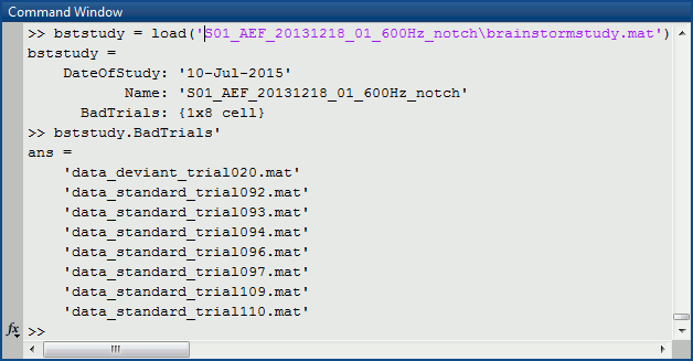
There is no field in the file structure that says if the trial is good or bad.
This information is saved at the level of the folder, in the brainstormstudy.mat file.Right-click on an imported folder > File > Show in file explorer.
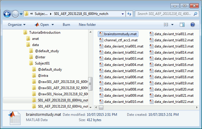
Load the brainstormstudy.mat file into Matlab, the bad trials are listed in the cell array "BadTrials":
Useful functions
in_bst_data(DataFile, FieldsList): Read an imported epoch.
in_bst(FileName, TimeWindow): Read any Brainstorm data file with the possibility to load only a specific part of the file. "TimeWindow" is a range of time values in seconds: [tStart, tStop].
bst_process('LoadInputFile', FileName, Target, TimeWindow): The most high-level function for reading data files. "Target" is a string with the list of sensor names or types to load.

