|
Size: 9245
Comment:
|
Size: 9305
Comment:
|
| Deletions are marked like this. | Additions are marked like this. |
| Line 11: | Line 11: |
| . {{attachment:HLUDisplay1.png||font-size="10pt"}} | . {{attachment:HLUDisplay1.png||height="314",width="389"}} |
| Line 14: | Line 14: |
| . {{attachment:HLUDisplay2.png}} | . {{attachment:HLUDisplay2.png||height="122",width="197"}} |
| Line 17: | Line 17: |
| . {{attachment:HLUTimeseries.png}} | . {{attachment:HLUTimeseries.png||height="280",width="637"}} |
Tutorial - Head Motion
All efforts should be made to avoid any movements and in particular head movements during a MEG recording, as it can cause various issues such as blurring of signals and loss of amplitude, mis-localization of source activity, and possibly motion artefacts. Yet it is important to evaluate and account for any head motion at the time of analysis. This is possible because the positions of the head tracking coils are saved in channels along the MEG data. It is important to note however that most analysis software, including Brainstorm, assume a single fixed position for the head for most computations. This "reference" position is the one that is measured just before the recording starts and that is saved separately from the continuous head localization channels.
This tutorial will explore different options on how to deal with head motion, using the sample_omega.zip dataset available on the download page. See MEG resting state & OMEGA database (CTF) for details on the BIDS specifications and how to load a MEG-BIDS dataset in Brainstorm. Note that importing all the subjects can take a while; for this tutorial, you can only import sub-0007.
Motion visualization
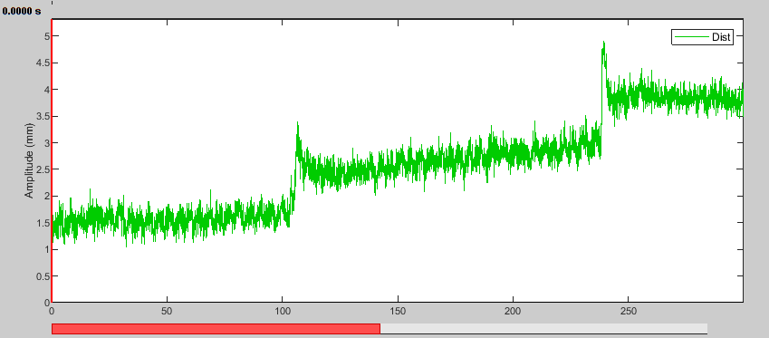
First, in order to evaluate the level of motion, we will display a special montage based on the head localization coils. This calculates the distance at each point in time with respect to the initial/reference head position. That distance is based on a sphere (approximating the head) attached to these head coils, thus accounting for all types of motion of all parts of the head equally.
After reviewing the raw data for subject sub-0007, right-click on the task-rest run > Switch epoched/continuous.
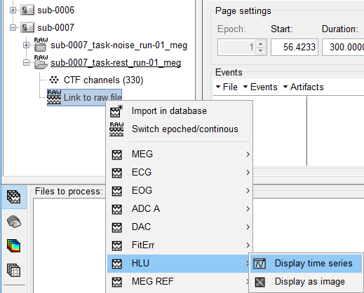
Right-click on the run again > HLU > Display time series.

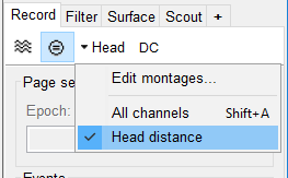
- On the Record tab, make sure DC is not selected (or you'll get a warning) and select the Head Distance montage.

- Set the Page settings duration to 300 seconds to see a good part of the recording at once. It may take a little time for the data to load.

Adjust the reference head position
Given that the default reference position is measured at the very beginning of the recording, we can improve co-registration by replacing it with one that better represents the position throughout.
Drag the raw recording to the Process1 tab and click Run. Select Process > Events > Adjust Head Position (CTF). Keep the default options, as below:
[screenshot]
Adjust head position to median location: This will adjust the co-registration between the MEG sensors and the digitized head coil positions. In Brainstorm terms, it is the "Dewar=>Native" transformation that is adjusted, but the adjustment is saved in the channel file as a separate "AdjustedNative" transformation properly placed right after "Dewar=>Native" and before any additional transformations such as the one created by "Refine using head points". The new reference head position is based on the geometric median of each localization coil positions throughout the recording. Note that it is safe to run this process multiple times. The correction will only be applied once.
Remove head position adjustment: This will undo the previous option. It will return the reference position to the default initial position.
Undo coregistration refinement using head points: While not exactly related to this process, this, similarly to the previous option, allows to undo "Refine using head points".
Display "before" and "after" alignment figures: This will open the same figure as "MRI registration > Check", both before and after the change selected above to visualize the adjustment.
- Run the process.
The figures don't show much difference for this recording, but we can notice a small drop looking at the LPA point and the head point near the back edge of the helmet. A message in the Matlab command window also tells us that the position changed by 3.7 mm.
[screenshot]
- Display the HLU time series again. The distance to the reference position is now reduced and closest in the middle of the recording.
[screenshot]
Mark head motion events
For long recordings, such as is typical for epilepsy, or when a large movement is present, a single head position may not be appropriate for the entire duration. In these cases, it may be preferable to split the recording in smaller segments where the head is stable and reject segments where too much motion is present. To do this, we first need to detect and mark these segments. Note that this process does not depend in any way on the reference position, so there is no need to adjust it first as we did.
There is not much motion in this dataset, so we will use extremely conservative thresholds to illustrate this process.
With the recording still in the Process1 tab, click Run. Select Process > Events > Detect head motion events (CTF). Use these settings:
[screenshot]
Movement threshold: For each segment, the head position distance from the first sample of the segment is measured. As soon as it exceeds this threshold, a new segment is created.
Minimum split length: If a segment is smaller than this length, it will be marked as BadHeadMotion. It represents segments where the displacement was too large and too fast.
Detect head coil fit errors: Along with their position, the head coil localization fit error is recorded. If this error is large, the position cannot be trusted. In practice, a bad fit often happens along with movement or a coil being too far from the helmet, i.e. a bad head position. However, it could also indicate that a head coil fell off of the subject, in which case the data might still be good.
Fit error tolerance: Segments where the error goes above this threshold will be marked as BadHeadFit.
- Run the process.
- Display the HLU time series one more time.
[screenshot]
In this first half of the dataset, we see one bad segment and three stable segments that correspond well with the jumps in the distance time series. We can also see these two new event groups in the Record tab. Note that it took a few tries with different thresholds and minimum durations to get the segments to fit that well.
Split the recording based on head motion events
We now can proceed to splitting our raw recording into segments with a stable head position.
Again, with the recording in the Process1 pane, click Run. Select Process > File > Split Raw File. Use the StableHead events we just created.
[screenshot]
Event name: Name of the extended event group to extract from the raw recording.
Keep segments outside of continuous event?: If this is selected, it will also produce files for any segment of the raw recording that is not included in one of the extended event selected. In our case, it would also extract the BadHeadMotion segments, which we don't need.
- Run the process.
A new condition appears in the database explorer for each extracted segment.
[screenshot]
We now should correct the reference position for each new raw file, otherwise the splitting would not achieve much.
- Clear the Process1 tab and add the 5 new raw conditions.
- Run the Adjust head position process.
Nothing seems to happen and the command window informs us that the head position was already adjusted. We must therefore undo the previous global adjustment (Remove head position adjustment) and apply it again to have an adjustment adapted to each segment. This can be done in one go by adding the Adjust head position process twice to our pipeline.
[screenshot]
- Select the recording of the first segment and display the HLU distance montage.
[screenshot]
We now see the head distance stays below half a mm until the end of the segment where it jumps to about 1.5 mm, close to our threshold. You can check that the other segments have similarly low remaining motion.
Head motion correction with SSS [TO DO]
Signal Space Separation (SSS) is a data cleaning technique that uses a spherical harmonic decomposition of the MEG signal to separate it into components originating from inside or outside the sensor shell. By reconstructing the signal with only the "inside" components, environmental interference is reduced.
The same spherical harmonic expansion can be used to correct for head motion by reconstructing the signal with new sensor locations adapted to the head position at each instant. (In the head coordinate system, head motion translates to motion of the sensor array.) In other words, we correct for head motion by interpolating the field at new sensor locations, using spherical harmonics for the interpolation.
The SSS process can therefore be used both for motion correction and signal cleaning, but here we will use it only for motion correction. In that case, the process takes care of selecting the expansion orders for inside and outside harmonics, using in total as many harmonics as sensors.
