MEG median nerve tutorial (CTF)

Authors: Francois Tadel, Elizabeth Bock, John C Mosher, Sylvain Baillet

The dataset presented in this tutorial was used in the previous generation of introduction tutorials. We kept it on the website as an additional illustration of data analysis, and as a comparison with median nerve experiments recorded with other MEG systems (Elekta-Neuromag, Yokogawa). No new concepts are presented in this tutorial. For in-depth explanations of the interface and theoretical foundations, please refer to the introduction tutorials.

Download and installation

• Requirements: You have already followed all the basic tutorials and you have a working copy of Brainstorm installed on your computer.

• Go to the Download page of this website, and download the file: sample_raw.zip

• Unzip it in a folder that is not in any of the Brainstorm folders (program folder or database folder).
• Start Brainstorm (Matlab scripts or stand-alone version).

• Select the menu File > Create new protocol. Name it "TutorialRaw" and select the options:

  • No, use individual anatomy,

  • No, use one channel file per run.

Import the anatomy

• Create a new subject Subject01.

• Right-click on the subject node > Import anatomy folder:

  • Set the file format: "FreeSurfer folder"

  • Select the folder: sample_raw/anatomy

  • Number of vertices of the cortex surface: 15000 (default value)

• Click on the link "Click here to compute MNI transformation".

• Set the 3 required fiducial points (indicated in MRI coordinates):
  • NAS: x=127, y=212, z=123
  • LPA: x=55, y=124, z=119
  • RPA: x=200, y=129, z=114

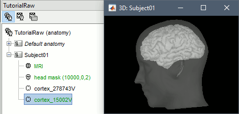
• At the end of the process, make sure that the file "cortex_15000V" is selected (downsampled pial surface, that will be used for the source estimation). If it is not, double-click on it to select it as the default cortex surface.
  
  

Link the recordings

• Switch to the "functional data" view (middle button in the toolbar above the database explorer).

• Right click on the Subject01 > Review raw file:

  • Select the file format: MEG/EEG: CTF

  • Select the folder: sample_raw/Data/subj001_somatosensory_20111109_01_AUX-f.ds

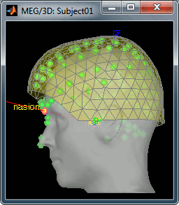
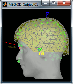
• Refine the registration with the head points: YES.
  
  

Pre-processing

Evaluate the recordings

• Drag and drop the "Link to raw file" into the Process1 list.

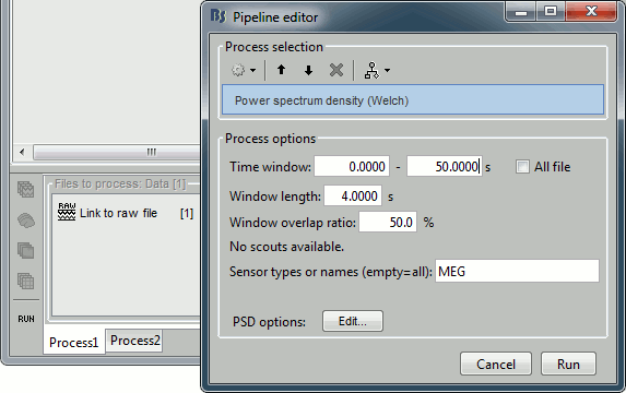
• Select the process "Frequency > Power spectrum density", configure it as follows:
  
  

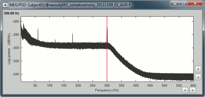
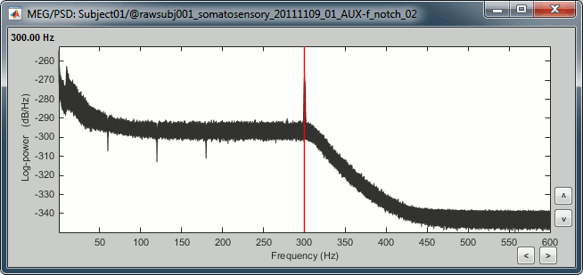
• Double-click on the PSD file to display it. It shows the estimate of the power spectrum for the first 50 seconds of the continuous file, for all the sensors, with a logarithmic scale. You can identify four peaks at the following frequencies: 60Hz, 120Hz, 180Hz and 300Hz. The first three are related with the power lines (acquisition in Canada, where the electricity is delivered at 60Hz, plus the harmonics). The last one is an artifact of the low-pass filter at 300Hz that was applied on the recordings at the acquisition time.
  
  

Remove: 60Hz and harmonics

• In Process1, keep the "Link to raw file" selected.

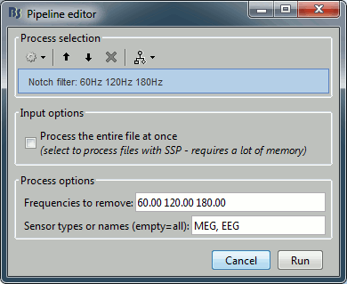
• Run Pre-process > Notch filter: Frequencies to remove = 60, 120, 180 Hz.
  
  

• To evaluate the results of this process, select the new filtered file ("Raw | notch") and run again the process "Frequency > Power spectrum density".
  
  

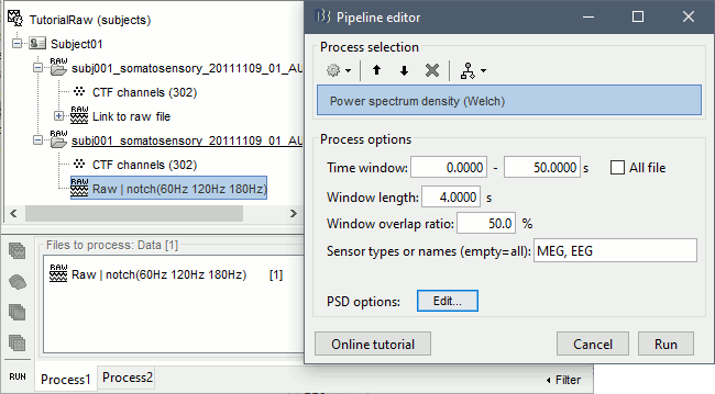
• You should observe a significant decrease of the contributions of the removed frequencies (60Hz, 120Hz, 180Hz) compared with the original spectrum.
  
  

Heartbeats and blinks

• Double-click on the filtered continuous file to display all the MEG recordings.

• Right-click on the link > ECG > Display time series, to look at the heartbeats.

• Right-click on the link > EOG > Display time series, to look at the eye movements.

• From the Artifacts menu in the Record tab, run the following detection processes:

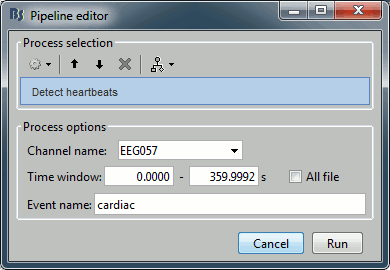
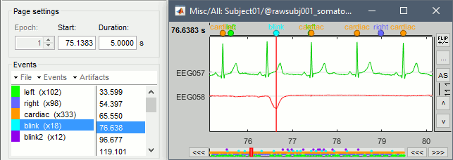
• Artifacts > Detect heartbeats: Select channel EEG057, event name "cardiac".
  
  

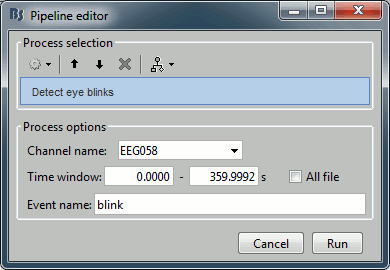
• Artifacts > Detect eye blinks: Select channel EEG058, event name "blink".
  
  

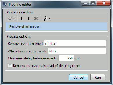
• Artifacts > Remove simultaneous: To avoid capturing ocular artifacts in the cardiac SSP.
  
  

• Review the traces of ECG/EOG channels and make sure the detected events make sense.
  
  

• Artifacts > SSP: Heartbeats: Event "cardiac", sensors="MEG".

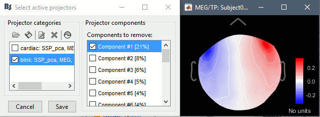
• Display the first three components: None of them are clearly related to a cardiac artifact. This can have two interpretations: the cardiac artifact is not very strong for this subject and the influence of the heart activity over the MEG sensors is completely buried in the noise or the brain signals, or the characterization of the artifact that we did was not so good and we should refine it by selecting for instance smaller time windows around the cardiac peaks. Here, it's probably due to the subject's morphology. Some people generate strong artifacts in the MEG, others don't.

• In this case, it is safer to unselect this "cardiac" category, rather than removing randomly spatial components that we are not sure to identify.
  
  

• Artifacts > SSP: Eyeblinks: Event "blink", sensors="MEG ", use existing SSP. (select component #1)
  
  

Epoching and averaging

Import the recordings

• Right-click on the filtered file "Raw | notch" > Import in dabase.
  
  

• The following figure appears, and asks how to import these recordings in the Brainstorm database.
  
  

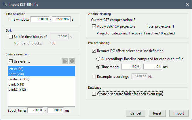
  • Time window: Time range of interest, keep all the time definition.

  • Split: Useful to import continuous recordings without events. We do not need this here.

  • Events selection: Check the "Use events" option, and select both Left and Right.

  • Epoch time: Time instants that will be extracted before an after each event, to create the epochs that will be saved in the database. Set it to [-100, +300] ms

  • Use Signal Space Projections: Use the active SSP projectors calculated during the previous pre-processing steps. Keep this option selected.

  • Remove DC Offset: Check this option, and select: Time range: [-100, 0] ms. For each epoch, this will: compute the average of each channel over the baseline (pre-stimulus interval: -100ms to 0ms), then subtract it from the channel at all the times in [-100,+300]ms.

  • Resample recordings: Keep this unchecked

  • Create a separate folder for each epoch type: If selected, a new folder is created for each event type (here, it would create two folders "left" and "right"). This option is mostly for EEG studies with channel files shared across runs. In a MEG study, we usually recommend to use one channel file per run, and to import all the epochs from one run in the same folder.

• Click on Import and wait. At the end, you are asked whether you want to ignore one epoch that is shorter than the others. This happens because the acquisition of the MEG signals was stopped less than 300ms after the last stimulus trigger was sent. Therefore, the last epoch cannot have the full [-100,300]ms time definition. This shorter epoch would prevent us from averaging all the trials easily. As we already have enough repetitions in this experiment, we can just ignore it. Answer Yes to this question to discard the last epoch.
  
  

• At this stage, you should review all the trials (press F3 to jump to the next file) to make sure that you don't have any bad trial that have been imported. If you find a bad trial: right-click on the file or on the figure > Reject trial.
  
  

Averaging

• Drag and drop all the left and right trials to the Process1 tab.

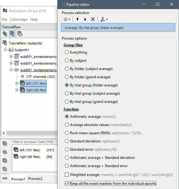
• Run the process Average > Average files > By trial group (folder average):
  
  

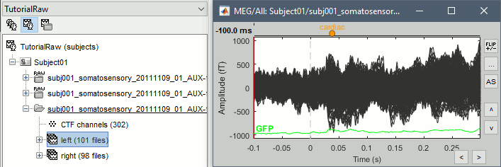
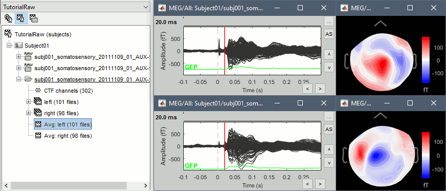
• Double-click on the Left and Right averages to display all the MEG sensors:
  
  

Stimulation artifact

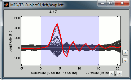
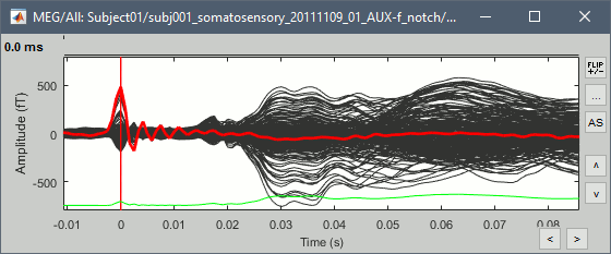
Zoom around 4ms. This sharp peak followed by fast oscillations is an artifact due to the electric stimulation device. In the stimulation setup: the stimulus trigger is initiated by the stimulation computer and sent to the electric stimulator. This stimulator generates an electric pulse that is sent to electrodes on the subject's wrists. This electric current flows in the wires and the in the body, so it also generates a small magnetic field that is captured by the MEG sensors. This is what we observe here at 4ms.

There is a 4ms delay before the stimulus is actually received by the subject, due to all the electronics in between, therefore everything is shifted by 4ms in the recordings. These hardware delays are unavoidable and should be quantified precisely before starting scanning subjects or patients. You have two options: either you remember it and subtract the delays when you publish your results, or you fix the files now by changing the time reference in all the files. Let's illustrate this second method now.

• Close all the figures, clear the Process1 list and drag and drop all the trials and all the averages (or simply the two left and right condition folders).

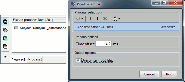
• Select the process "Pre-process > Add time offset". Set the time offset to -4.2 ms, to bring back this stimulation peak at 0ms. Select also the "Overwrite input files" option.
  
  

• This fixes the individual trials and the averages. Double-click on the "Avg: left" file again to observe that the stimulation artifact is now occurring at 0ms exactly, which means that t=0s represents the time when the electric pulse is received by the subject.

Explore the average

Open the time series for the "Avg: left". Then press Control+T, to see on the side a spatial topography at the current time point. Then observe what is happening between 0ms and 100ms. Start at 0ms and play it like a movie using the arrow keys left and right, to follow the brain activity millisecond by millisecond:

• 16 ms: First response, the sensory information reaches the right somatosensory cortex (S1)

• 30 ms: Stronger and more focal activity in the same region, but with a source oriented in the opposite direction (S1)

• 60 ms: Activity appearing progressively in a more lateral region (S1 + S2)

• 70 ms: Activity in the same area in the left hemisphere (S2 left + S2 right)
  
  

Source analysis

We need now to calculate a source model for these recordings, using a noise covariance matrix calculated from the pre-stimulation baselines. This process is not detailed a lot here because it is very similar to what is shown in the CTF-based introduction tutorials.

Head model

We need now to calculate a source model for these recordings, using a noise covariance matrix calculated from the pre-stimulation baselines. This process is not detailed a lot here because it is very similar to what is shown in the CTF-based introduction tutorials.

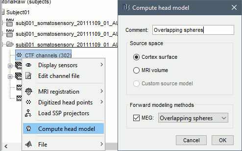
• Right-click on the channel file > Compute head model. Keep the default options.

• For more information: Head model tutorial.

Noise covariance matrix

• Select all the Left and Right trials, right-click > Noise covariance > Compute from recordings. Baseline = [-104, -5]ms
  
  

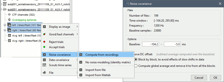
• Leave all the default options and click [OK].

• For more information: Noise covariance tutorial.

Inverse model

• Right-click on the headmodel > Compute sources. Select dSPM and all the default options. This will run a source reconstruction grouping the information from the magnetometers and the gradiometers into the same model. This is the recommended procedure, but you can also estimate sources for the two types of sensors separately if needed.
  
  

• A shared inversion kernel is created in the (Common files) folder, and a link node is now visible for each recording file, single trials and averages.

• For more information: Source estimation tutorial.

Scouts

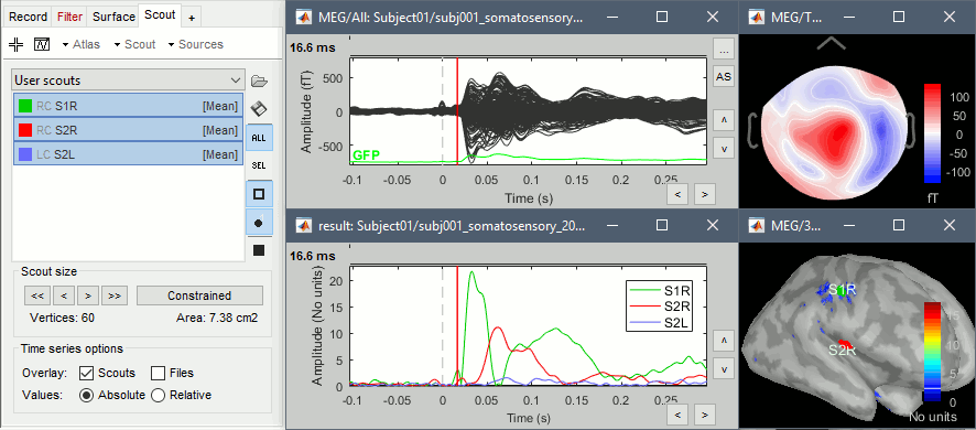
Place scouts to capture the activity in the primary and secondary somatosensory areas to track the processing of the electric stimulations in time, at the surface surface of the brain. When reviewing the average for the left condition, you can use the following times and thresholds:

• S1R: t=16ms, threshold=20%

• S2R: t=60ms, threshold=80%

• S2L: t=60ms, threshold=60%
  
  

Scripting

The following script from the Brainstorm distribution reproduces the analysis presented in this tutorial page: brainstorm3/toolbox/script/tutorial_raw.m