|
Size: 22551
Comment:
|
Size: 22774
Comment:
|
| Deletions are marked like this. | Additions are marked like this. |
| Line 142: | Line 142: |
| === Types of correlation === In general brain annotations consist of only-one time sample. So it does not change with time. However, this is necessarily the case of the brain activity maps (source maps) that we want to compare. As such the bst-neuromaps plugin allows comparisons between map A and maps B that can have different number of time samples as follows: * A: 1-sample source estimation × B: 1-sample source estimation (or brain annotation) This gives as result one value that is the correlation between the maps * A: N-sample source estimation × B: 1-sample source estimation (or brain annotation) This gives as result one correlation value for each time point in the sic * A: N-sample source estimation × B: N-sample source estimation This gives as result one correlation value for each time point, thus it is possible to visualize the evolution of the similarities between source maps. While spatial autocorrelation is handled for each time point, temporal autocorrelation is corrected. |
=== Spatial correlation === Spatial correlation is performed between two brain maps, A and B, which can be time-defined, i.e., comprise more than one time sample. In the case of brain annotations, they consist of only-one time sample. However, this is necessarily the case of the brain activity maps (source maps). Thus, when performing spatial correlations, depending on the number of time samples in maps A and B there are three possible scenarios: * '''Map A''': 1 time sample × '''Map B''': 1 time sample (e.g., brain annotation) This gives as result '''one''' value that is the correlation between the maps * '''Map A''': N time samples × '''Map B''': 1 time sample (e.g., brain annotation) This gives as result N correlation values, one for each correlation between the N time samples in map A and the 1 time sample in map B. * '''Map A''': N time samples × '''Map B''': N time samples This gives as result N correlation values, one for each correlation between the `i` time sample in map A and the `i` time sample in map B. Thus, it is possible to visualize the evolution of the similarities between source maps. While spatial autocorrelation is handled for each time point, temporal autocorrelation is corrected. |
Neuromaps plugin
Authors: Le Thuy Duong Nguyen, Raymundo Cassani
Please note that this tutorial page is currently under construction.
The neuromaps plugin for Brainstorm (bst-neuromaps) integrates curated brain annotations (also referred to as brain maps) and tools to further expand the accessibility and inclusivity of brain-mapping tools, as part of an Open Science initiative. We extend these pioneering tools to the Brainstorm environment for users without any prior computer programming experience, providing an intuitive graphic user interface. This approach eliminates barriers of entry for researchers, fostering a more inclusive research community.
The present tutorial will demonstrate the plugin’s functionality within the Brainstorm interface; for a detailed breakdown of the algorithm, please refer to the neuromaps plugin GitHub.
Contents
Introduction
Neuromaps is a Python toolbox designed for assessing, transforming, and analyzing structural and functional brain annotations (Markello, Hansen et al., 2022). It marks a significant stride towards integrative analytics in multimodal, multiscale neuroscience by bridging the gap between various neuroimaging modalities and proposing analytical tools to establish connections among different brain features. The toolbox comprises a curated repository of brain annotations in their native space, methods for generating transformations across multiple coordinate systems, and offers a systematic workflow for comprehensive structural and functional annotation enrichment analysis of the human brain.
With the bst-neuromaps plugin we aim to bring annotations from the neuromaps toolbox in to Brainstorm, and provide additional methods for their analysis. The plugin takes advantage of the Brainstorm GUI to enhance accessibility, especially for researchers who may not be familiar with command-line interfaces or programming languages such as Python.
For the first iteration of the implementation of the bst-neuromaps plugin, we focused on the neurotransmitter receptors and transporters. Twenty-six different annotations from the neuromaps toolbox were selected, covering nine different neurotransmitter systems: acetylcholine, cannabinoid, dopamine, GABA, glutamate, histamine, norepinephrine, opioid, and serotonin. These brain annotations are sourced from open-access repositories, addressing the need for a comprehensive tool that integrates standardized analytic workflows for neuroimaging data.
Key features
Flexible framework designed to accommodate future expansions and updates.
Repository of precomputed annotations sourced from the published literature, ensuring accessibility and ease of use.
All the information for these maps, including the appropriate citations to use can be found in this spreadsheet.
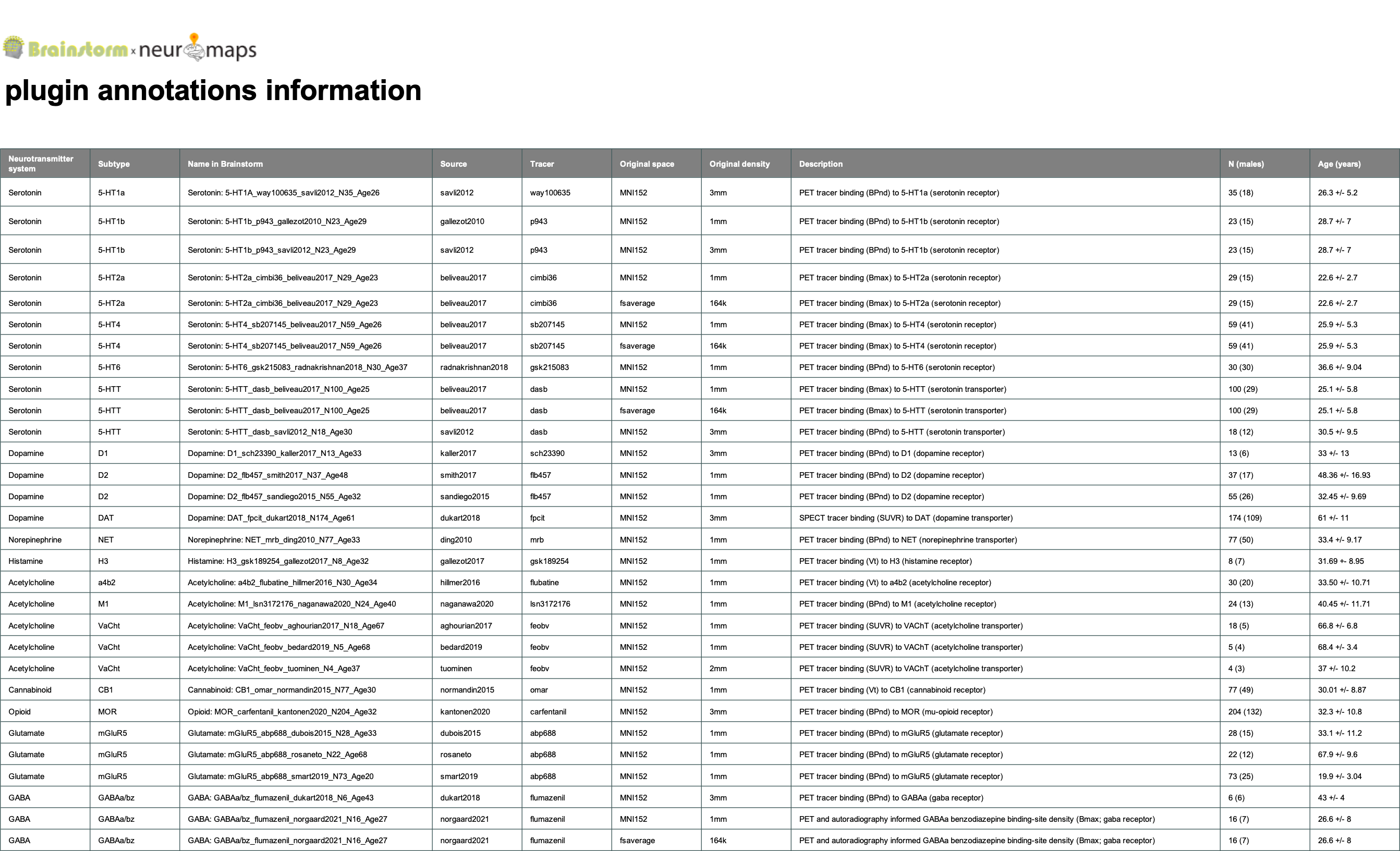
To obtain the surface annotations, the original (volume) annotations offered in MNI152 space were transformed to FsAverage using the registration fusion framework proposed in neuromaps (Buckner et al., 2011; Wu et al., 2018).
Correlation processes featuring spatially informed null models that account for spatial autocorrelation.
Install
Being a Brainstorm plugin, the bst-neuromaps plugin can be installed, updated and removed directly from the Brainstorm GUI. For further information, see the plugins tutorial.
From the main window go to Plugins > Anatomy > neuromaps > Install.
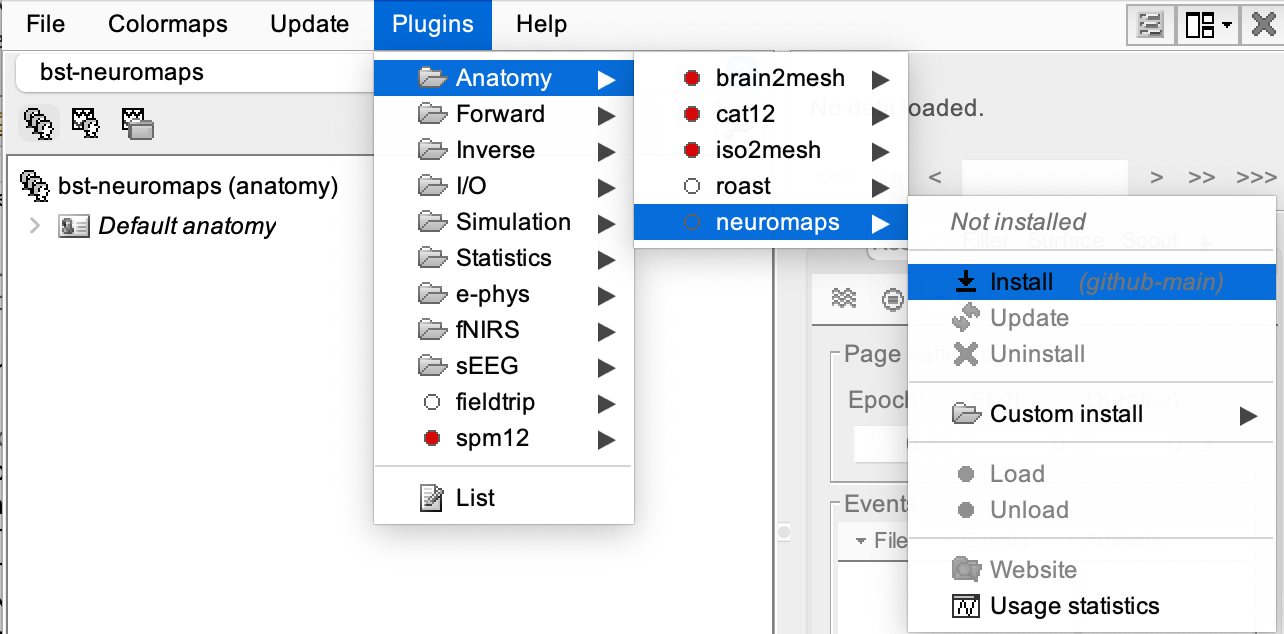
A message will appear saying, "Plugin neuromaps is not installed on your computer. Download the latest version of Neuromaps now?" click 'Yes'.
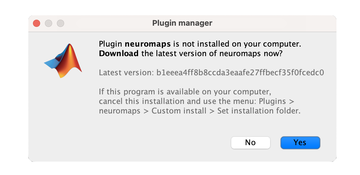
- The plugin will be downloaded and installed automatically. Once installed, you will see a confirmation message.
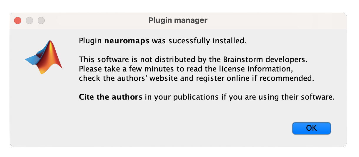
The README file will appear; after thoroughly reviewing it, click on the "I agree" button to confirm your acceptance of the plugin's terms and conditions.
By following these steps, you will successfully install the bst-neuromaps plugin.
Importing brain annotations
Click on the [Run] button at the bottom-left corner of the Process1 tab.
When the Pipeline editor window appears, click on the first button in the toolbar under 'Process selection' (the one with a gear icon). It will show you a list of processes.
Go to Sources > Fetch brain annotations from neuromaps.
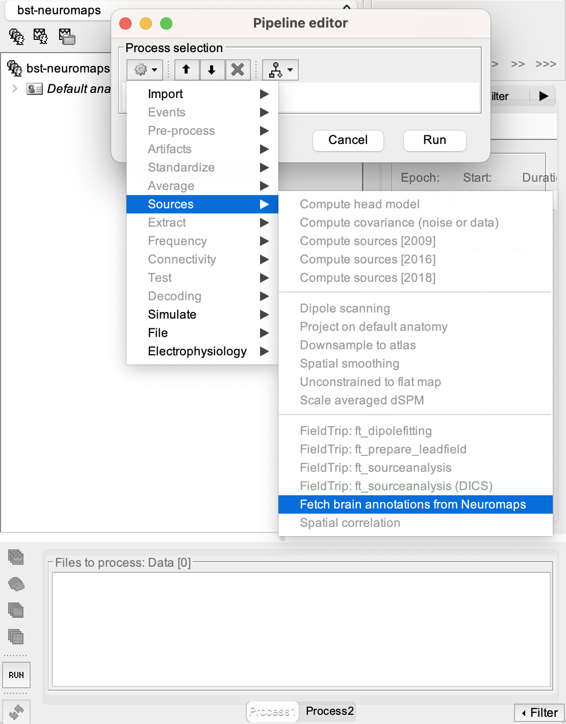
The brain annotations will be listed right under, in the name format
[neurotransmitter]:[subtype]_[tracer]_[source]_[size]_[age]
for example:
Dopamine: D1_sch23390_kaller2017_N13_Age33'Select all the maps you want to import and click Run.
Visualizing brain annotations
Once you have fetched the brain annotations, a new subject Neuromaps which uses the default FsAverage anatomy will appear in the Brainstorm database.
All the imported brain annotations will be visible in the Functional data in the Neuromaps subject. Brain annotation are grouped in folders according to the neurotransmitter.
To visualize the surface annotations, you can either double-click on the file or right-click > Cortical activations > Display on cortex.
- You can double-click the color bar at the bottom right of the resulting window to better visualize the annotations (this resets the values to default).
Visualization capabilities
Implementing neuromaps directly into Brainstorm further enhances the overall user experience by providing greater flexibility and control over the visualization and analysis of brain annotations. Brainstorm's advanced functionalities allow users to effortlessly rotate the brain annotations, zoom in and out, reposition them, obtain the coordinates for any point, take snapshots, adjust the transparency, and more.
The ‘Surface’ tab of the Brainstorm window contains buttons and sliders to control the display of these surfaces. Additional relevant functionalities, as outlined in Tutorial 3: Display the Anatomy, include:
Smooth: Inflates the surface to make all the parts of the cortex envelope visible.This is just a display option, it does not actually modify the surface.
Resect: The sliders and the buttons Left/Right/Struct at the bottom of the panel allow you to cut the surface or reorganize the anatomical structures in various ways.
Edge: Display the faces of the surface tesselation.
Colormap
The default colormap upon opening the brain annotation is royal_gramma, but you have the option to set it to other sequential, diverging, or rainbow colormaps. Simply right-click on the brain annotation window, navigate to Colormap: Sources > Colormap.
If you modify a colormap, the changes will be applied to all the figures, saved in your user preferences and available the next time you start Brainstorm. If you wish to undo the changes and reset the colormap to its default values, click on Restore defaults or double-click on the color bar.
You also have the opportunity to customize the brightness, contrast, and decide the color mapping, among other settings. For a comprehensive list of available options with detailed instructions, please refer to Tutorial 18: Colormaps.
Creating weighted-averaged brain annotations
Neurotransmitter annotations that have the same tracer (e.g., Serotonin: 5-HT1b_p943_gallezot2010_N23_Age29 and Serotonin: 5-HT1b_p943_savli2012_N23_Age29 have the same p943 tracer) can be combined to obtain a larger sample size for your analysis. To accomplish this, you can perform a weighted average. In the same way you selected the fetching process:
- Drag-and-drop all the relevant brain annotation files into the processing pipeline (Process1). In this example, we will select the two 5-HT1b files mentioned.
Click on the [Run] button at the bottom-left corner of the Process1 tab.
Once the Pipeline editor window appears, click on the first button in the toolbar under 'Process selection' (the one with a gear icon).
Select the process Average > Average files.
Under 'Group files,' select Everything and for 'Function,' Arithmetic average: mean(x).
- Check the 'Weighted average' box, as shown below.
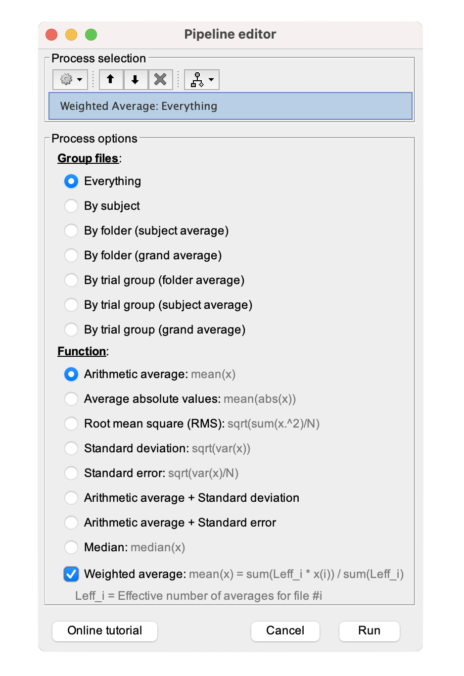
Click Run. A new file WAvg: 2 files will be added under the same neurotransmitter folder.
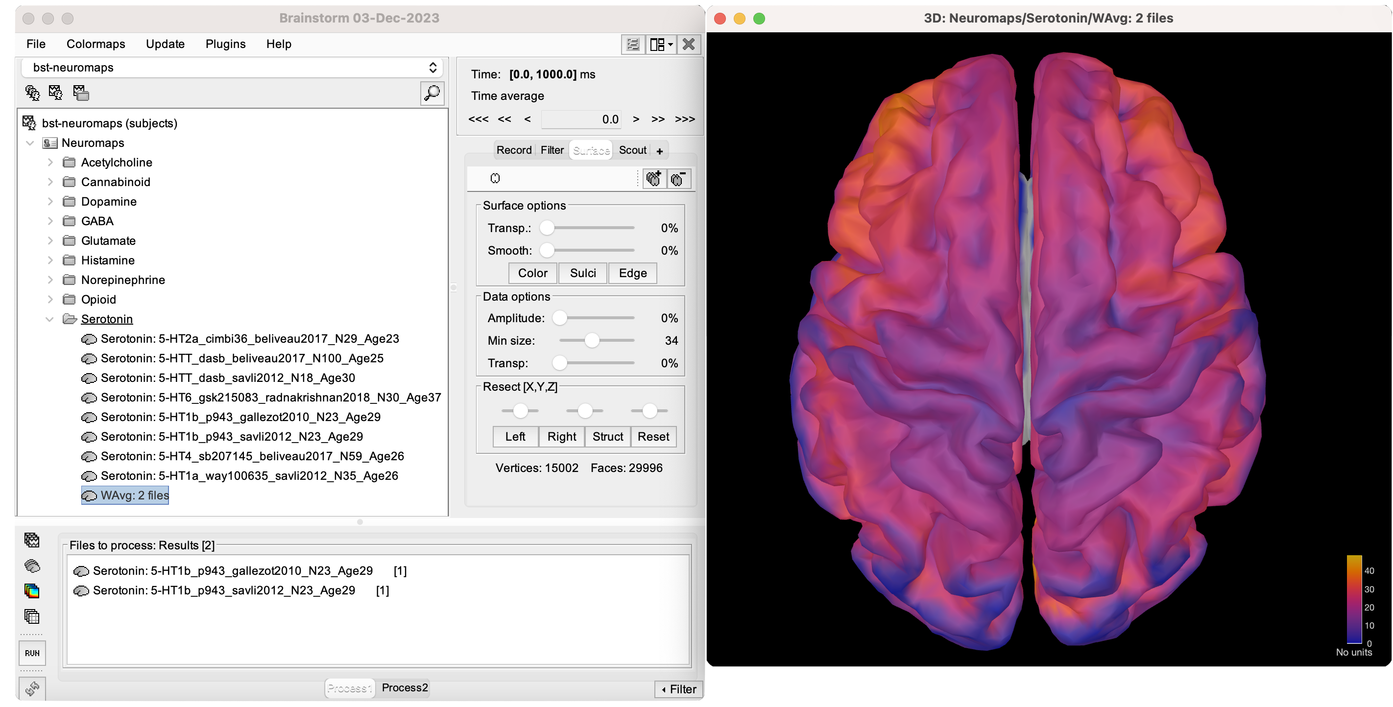
To visualize this new weighted-averaged annotation, follow the same steps as with any brain annotation. Either double-click on the file or right-click > Cortical activations > Display on cortex.
By default, the new weighted-averaged file is named WAvg: followed by the number of files averaged. If you wish to rename this or any other file to provide more informative labels for your analysis, follow these steps:
- Click once on the file to select it.
- With a right-click (or pressing F2), you will enter renaming mode and the file name will become editable.
- Type in the new desired name for the file.
- Press the "Enter" key on your keyboard or click outside the file name to save the new name.
Alternatively, you can right-click > File > Rename.
Parcellations
Parcellations are know as Scouts in the Brainstorm jargon. Please refer to Tutorial 23: Scouts for a more in-depth guide in creating, manipulating, and analyzing scouts for effective exploration and comparison of brain activity across different experimental conditions and regions of interest. The figure below shows the left and top views of the brain annotation Dopamine: D1_sch23390_kaller2017_N13_Age33 without and with different cortical parcellations. Only the borders of the Scouts are shown to avoid distorting the underlying color.
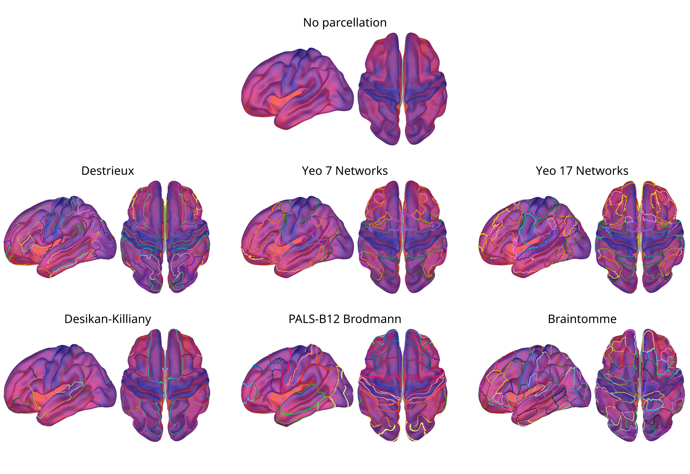
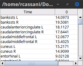
So far our annotations have a value for each vertex on the cortical surface. However, it is common to summarize the these values using Scouts. To do so it is possible to use the Extract > Scout time series as
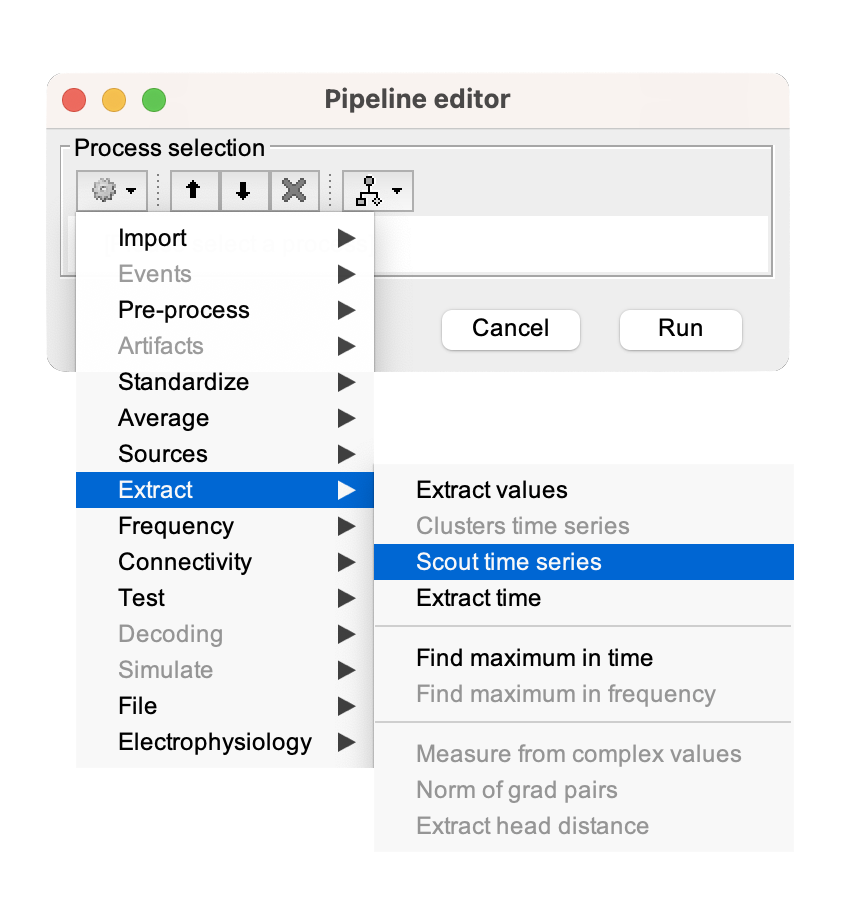
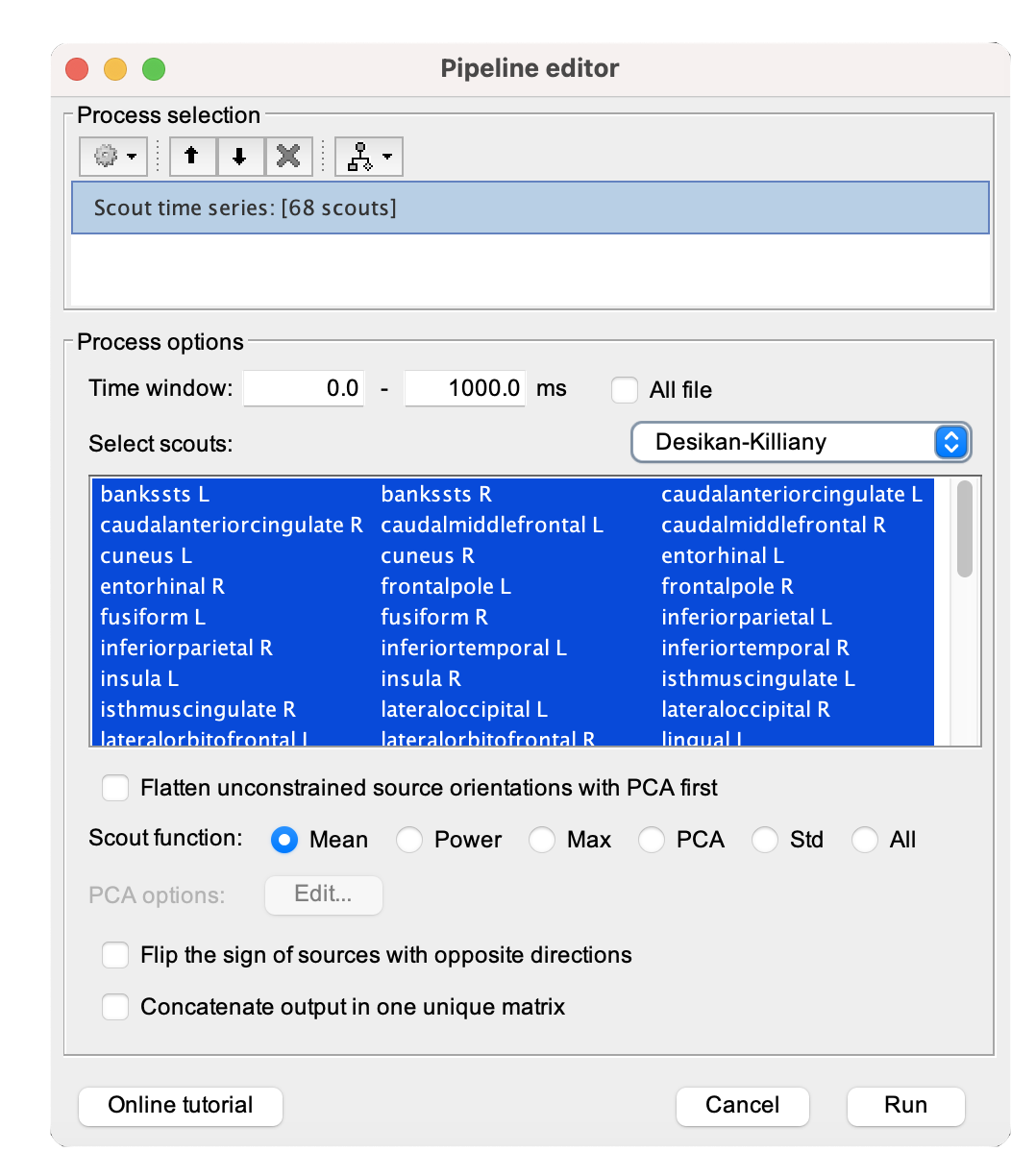
The result is a matrix file (ICON) with one value for Scout.
Statistical analysis
One of the main advantages of having these brain annotations in a common coordinate system is that we can statistically compare (spatial correlation) their spatial topographies. However, most statistical analyses (e.g., Pearson correlation) assume that the values of observations in each sample are independent of one another. Spatial autocorrelation violates this assumption because samples taken from nearby areas are related to each other and are not independent. Spatially-naive null models, both parametric and non-parametric, yield inflated p-values and are inappropriate for significance testing of neuroimaging brain maps. When applied to spatially-autocorrelated brain maps typical of most neuroimaging data, these models approach a false positive rate higher than 75% and their usage in the field is discouraged (Markello, R. D., & Misic, B., 2021). We therefore use spatially informed null models to benchmark the statistical unexpectedness of specific features of interest.
Spin test
Building on previous studies that assess the accuracy and computational efficiency of these models, we have selected the non-parametric method as the default for surface data and implemented the most widely adopted of these approaches, which involves randomizing the anatomical alignment between two cortical surface maps through spherical rotation by a random angle. This method is also know as spin-test, where each "spin" is a randomized rotation between the cortical maps (Alexander-Bloch et al., 2018).
According to the literature, null models converge quickly, reaching stable statistical estimates after approximately 100–500 nulls (Markello, R. D., & Misic, B. 2021). Researchers can use this information to balance accuracy and computational feasibility when determining the number of nulls for their analysis. Our recommendation is to generate 1000 nulls to establish a reliable null distribution of correlation coefficients and to estimate the two-tailed p-value for the original correlation between the pair of maps.
A spatial null model is enabled by default to encourage their broader adoption but users can easily revert to an uncorrected correlation by setting the number of spins (nulls) to zero.
[TODO] image to example of spin test.
Spatial correlation
Spatial correlation is performed between two brain maps, A and B, which can be time-defined, i.e., comprise more than one time sample. In the case of brain annotations, they consist of only-one time sample. However, this is necessarily the case of the brain activity maps (source maps). Thus, when performing spatial correlations, depending on the number of time samples in maps A and B there are three possible scenarios:
Map A: 1 time sample × Map B: 1 time sample (e.g., brain annotation)
This gives as result one value that is the correlation between the maps
Map A: N time samples × Map B: 1 time sample (e.g., brain annotation)
- This gives as result N correlation values, one for each correlation between the N time samples in map A and the 1 time sample in map B.
Map A: N time samples × Map B: N time samples
This gives as result N correlation values, one for each correlation between the i time sample in map A and the i time sample in map B. Thus, it is possible to visualize the evolution of the similarities between source maps. While spatial autocorrelation is handled for each time point, temporal autocorrelation is corrected.
Example
This are based on the results of the introduction tutoprial. Please follow it, at least until tutorial XX.
We will exemplify the use of the process in the bst-neuromaps plugin.
Spatial correlation with brain annotations
- [TODO] Using tutorial data. [TODO] Describe process GUI
The result is an statistical file, see the options in here.
Spatial correlation with any files
- [TODO] Using tutorial data, correlation of activity between diff stimulus. Show that activations are common around X ms. [TODO] Describe process GUI
The result is an statistical file, see the options in here.
On the hard drive
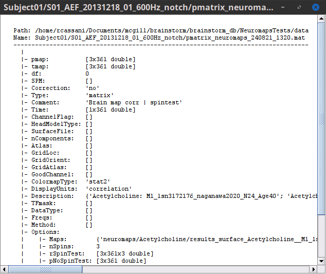
The resulting file is an matrix statistic file (), as such follows the same organization as described in here.
Right click on the stat matrix file that results from running spatial correlations > File > View file contents.
Description of the fields
pmap: [Nsignals x Ntime]: p-values for all the time points. If a spin test was performed these are the spin-test corrected p-values.
tmap: [Nsignals x Ntime]: values for correlation.
Correction: Correction for multiple comparison already applied ('no', 'cluster', 'fdr', ...)
Type: Type of the data ('matrix').
Comment: String displayed in the database explorer to represent the file.
Time: Time vector associated with the results.
Description: Each of the Comments for the files what where correlated.
History: Indicates the process and input file that gave origin to this stat matrix file.
Options: Specific fields for spatial correlation:
Maps: File names for the brain annotations
nSpins: Number of spins for the spin test. If 0 there was not spin test.
rSpinTest: [Nmaps x Ntime x Nspin] Correlation values for each of the spins for the spin test.
pNoSpinTest: [Nmaps x Ntime] p-values for no spin test.
Useful functions
process_np_fetch_maps*: Imports brain annotations into a "Neuromaps" Subject
process_np_source_corr1*: Spatial correlation between surface source maps and brain annotations
process_np_source_corr2*: Computes the spatial correlation between two sets of surface source maps
process_extract_pthresh: Mask the correlation values according to a significance level. It also applies correction for multiple comparisons.
* These processes are part of the bst-neuromaps plugin.
Applications for integrative research
The bst-neuromaps plugin opens up new and exciting avenues for research and can help address questions that depend crucially on anatomical localization. Below, we explore some potential uses of the plugin in advancing integrative research, supported by examples from the literature.
Annotating structural connectomes
Hansen, J. Y., Shafiei, G., Voigt, K., Liang, E. X., Cox, S. M., Leyton, M., ... & Misic, B. (2023). Integrating multimodal and multiscale connectivity blueprints of the human cerebral cortex in health and disease. Plos Biology, 21(9), e3002314.
- With the advancements in neuroimaging techniques, which enables the simultaneous exploration of diverse interregional relationships across spatial and temporal scales, neuromaps emerge as an invaluable tool for advancing integrative research in connectomics. The researchers noted a consistent primacy of molecular connectivity modes, demonstrating the mapping of correlated receptor similarity onto multiple phenomena. The use of neuromaps revealed both the similar and complementary ways in which connectivity modes reflect cortical geometry, structure, and disease and assisted in constructing a multimodal wiring map.
Identification of specific neurochemical targets for potential future clinical treatments
da Silva Castanheira, J., Wiesman, A. I., Hansen, J. Y., Misic, B., Baillet, S., Network Quebec Parkinson, & PREVENT-AD Research Group. (2023). Neurophysiological brain-fingerprints of motor and cognitive decline in Parkinson’s disease. medRxiv.
- Subject-level data can be contextualized against the brain annotations contained in the plugin to produce a subject-specific ‘fingerprint’ of how individuals express different structural and functional brain phenotypes. The authors were able to show the topographical alignment between spectral brain-fingerprints, the functional hierarchy of cortex, and neurotransmitter systems.
Wiesman, A. I., da Silva Castanheira, J., Degroot, C., Fon, E. A., Baillet, S., Network, Q. P., & Prevent-Ad Research Group. (2023). Adverse and compensatory neurophysiological slowing in Parkinson’s disease. Progress in Neurobiology, 231, 102538.
- Neuromaps has the potential to enhance the integration of neurophysiological and neurochemical data for a more comprehensive understanding of brain function, and assist in the identification of specific neurochemical targets for potential future clinical treatments. The authors demonstrated, for instance, that the clinical relationships of neurophysiological slowing in patients with Parkinson's disease are aligned topographically with the densities of selective neurotransmitter systems and the organization of sensory-association areas—namely, dopamine, serotonin, GABA, and norepinephrine systems.
Acknowledgements
The conception of the original neuromaps algorithm is due to Ross D. Markello, Justine Y. Hansen, Zhen-Qi Liu, Vincent Bazinet, Golia Shafiei, Laura E. Suárez, Nadia Blostein, Jakob Seidlitz, Sylvain Baillet, Theodore D. Satterthwaite, M. Mallar Chakravarty, Armin Raznahan & Bratislav Misic. The appropriate citation for neuromaps is as follows:
Markello, R.D., Hansen, J.Y., Liu, ZQ. et al. neuromaps: structural and functional interpretation of brain maps. Nat Methods 19, 1472–1479 (2022).
If you used any of the included maps, please also cite the original papers that publish the data. References for each map can be found in this spreadsheet.
- If you used the surface maps which were transformed using the registration fusion framework, please also cite:
Wu, J. et al. Accurate nonlinear mapping between MNI volumetric and FreeSurfer surface coordinate systems. Hum. Brain Mapp. 39, 3793–3808 (2018).
Contributing
We welcome contributions from the community to help improve and expand the functionality of the Neuromaps plugin. Feel free to submit pull requests on the GitHub repository, report issues, or provide suggestions below! Your feedback is invaluable in ensuring a user-friendly experience for researchers worldwide. We believe that open science is most impactful when the countless everyone is provided with equal access to the newest and greatest resources in the field.

