|
Size: 11623
Comment:
|
Size: 11225
Comment:
|
| Deletions are marked like this. | Additions are marked like this. |
| Line 4: | Line 4: |
| The Brainstorm window includes a graphical batching interface. With the two tabs Process1 and Process2 in the lower part of the window, you can easily select files from the database explorer and assemble a processing pipeline. Most of the operations available in the interface can also be executed this way, including everything we've been doing with Brainstorm so far. | The Brainstorm window includes a graphical batching interface. With the two tabs Process1 and Process2 in the lower part of the window, you can select files from the database explorer and assemble a processing pipeline. Most of the operations available in the interface can also be executed this way, including everything we've been doing with Brainstorm so far. |
| Line 6: | Line 6: |
| On the other hand, some features are only available this way. It is the case for the frequency filters we will need for the pre-processing of our auditory recordings. This tutorial is a parenthesis to explain how to select files and run processes on them, the cleaning of the recordings will resume in the next tutorial. | On the other hand, some features are only available this way. It is the case for the frequency filters we will need for the pre-processing of our auditory recordings. This tutorial is a parenthesis to explain how to select files and run processes, we will resume with the cleaning of the recordings in the next tutorial. |
| Line 14: | Line 14: |
| * You will see that it accepts all the folders and all the recordings, but not the channel file. * When you add a new node, the interface evaluates the number of files of the selected type that each of them contain. The number in the brackets next to each node represents the number of data files that where found in of them. * On top of the box, a comment shows the total number of files that are currently selected. <<BR>><<BR>> {{attachment:process1_example.gif}} * The buttons on the left side allow you to select what type of file you want to process: Recordings, sources, time-frequency, other. When you select another button, all the counts are updated to reflect the number of files the selected type that are found for each node. * Right now, if you select another file type, it would show only "0" everywhere because there are no sources or time-frequency decompositions available in the database yet. <<BR>><<BR>> {{attachment:process1_sources.gif}} |
* You will see that it accepts all the folders and all the recordings, but not the channel files. * When you add a new node, the interface evaluates the number of files of the selected type that each of them contain. The number in the brackets next to each node represents the number of data files that where found in them. * On top of the list, a comment shows the total number of files that are currently selected. <<BR>><<BR>> {{attachment:process1_example.gif}} * The buttons on the left side allow you to select what type of file you want to process: Recordings, sources, time-frequency, other. When you select another button, all the counts are updated to reflect the number of files of the selected type that are found for each node. * Right now, if you select another file type, it would show only "0" everywhere because there are no sources or time-frequency decompositions available in the database yet. <<BR>><<BR>> {{attachment:process1_sources.gif||height="159",width="464"}} |
| Line 21: | Line 21: |
| * Select the nodes to remove (holding Shift or Ctrl key) and press the '''Delete''' key. | |
| Line 23: | Line 24: |
| * Select the nodes to remove (holding Shift or Ctrl key) and press the '''Delete''' key. | == Filter by name or comment == When you have lots of files in a folder, like multiple source reconstructions or time-frequency files for each trial, it is difficult to grab just the ones you are interested in. After selecting your folders in the Process1 box, you can refine the selection with the '''Filter search box''' at the bottom-right corner of the window. |
| Line 25: | Line 27: |
| == Filter the files by name or comment == When you have lots of files in a folder, like multiple source reconstructions of time-frequency files for each trial, it is difficult to grab just the ones you are interested in. After selecting your files in the Process1 box, you can refine the selection by entering something in the '''Filter search box''' at the bottom-right of the Brainstorm window. |
* The example below shows how select the data file corresponding to the noise recordings: by typing "Noise" in the search box and selecting the option "Search file names". We cannot perform the search "by comment" because all the data files have the same comment "Link to raw file".<<BR>><<BR>> {{attachment:process1_search.gif||height="148",width="436"}} |
| Line 28: | Line 29: |
| The example below shows how select the data file corresponding to the noise recordings: by typing "Noise" in the search box and selecting the option "Search file names". We cannot perform the search "by comment" because all the data files have the same comment "Link to raw file". {{attachment:process1_search.gif}} Reminder: To see the file name corresponding to a node in the database, leave your mouse over it for a few seconds. You can do this both in the database explorer and the Process1 list. {{attachment:process_filename.gif}} |
* Reminder: To see the file name corresponding to a node in the database, leave your mouse over it for a few seconds. You can do this both in the database explorer and the Process1 list.<<BR>><<BR>> {{attachment:process_filename.gif||height="148",width="490"}} |
| Line 45: | Line 40: |
| == Running a process == 1. Click on Run. The Process selection window appears, with which you can create an analysis pipeline (ie. a list of process that are applied on the selected files one after the other). The first button in the toolbar shows the list of processed that are currently available. If you click on a menu, it's added to the list. . {{http://neuroimage.usc.edu/brainstorm/Tutorials/TutProcesses?action=AttachFile&do=get&target=pipeline1.gif|pipeline1.gif|class="attachment"}} 1. Some menus appear in grey (example: Sources > Spatial smoothing). This means that they are not meant to be applied to the type of data that you have in input, or at the end of the current pipeline. The "spatial smoothing" process may only be run on source files. 1. When you select a process, a list of options specific to this process is shown in the window. * To delete a process: Select it and press the ''Delete'' key, or the big cross in the toolbar. * With the "up arrow" and "down arrow" buttons in the toolbar, you can move up/down a process in the pipeline. 1. Now add the following processes, and set their options: * '''Pre-process > Band-pass filter''': 2Hz - 30Hz * In some processes, you can specify the type(s) of sensors on which you want to apply the process. This way you can for instance apply different filters on the EEG and the MEG, if you have both in the same files. * '''Extract > Extract time''': 40.00ms - 49.60ms, overwrite initial file * This will extract from each file a small time window around the main response peak. * Selecting the overwrite option will replace the previous file (bandpass), with the output of this process (bandpass+extract). This option is usually unselected for the first process in the list, then selected automatically. * '''Average > Average over time''': Overwrite initial file * Compute the average over this small time window. {{http://neuroimage.usc.edu/brainstorm/Tutorials/TutProcesses?action=AttachFile&do=get&target=pipeline2.gif|pipeline2.gif|class="attachment"}} 1. Save your pipeline: Click on the last button in the toolbar > Save > New... > Type "process_avg45". |
== Selecting processes == * Clear the file list and the search filters. * Select all the three datasets we have linked to our protocol. You can select the three "link to raw file" nodes, the three folders or the entire subject node. * Click on the '''[Run]''' button at the bottom-left corner of the Process1 tab. * The '''Pipeline editor''' window appears. You can use it to create an analysis pipeline, ie. a list of process that are applied on the selected files one after the other. The first button in the toolbar shows the list of processes that are currently available. If you click on a menu, it's added to the list. * Some menus appear in grey. This means that they are not meant to be applied to the type of data that you have in input, or at the end of the current pipeline. * In the current example, we have a file with the type "continuous raw recordings", so we have access mostly to menus to manipulate event markers, run cleaning procedures and import data blocks. You can recognize a few operations that we execturd in the previous tutorials: "Event > Read from channel" and "Event > Detect analog triggers". <<BR>><<BR>> {{attachment:process1_addprocess.gif||height="480",width="473"}} * When you select a process, a list of options specific to this process is shown in the window. * To delete a process: Select it and press the '''Delete''' key, or use the '''[X]''' button in the toolbar. * After selecting a first process, you add another one. The output of the first process will be passed to the second process without giving back the control to the user. This is how you can build a full analysis pipeline with the interface. |
| Line 63: | Line 51: |
| == Creating a pipeline == === Saving/exporting a pipeline === The last button in the the toolbar offers a list of menus to save, load and export the pipelines. |
* After adding a few processes, you can move up/down a process in the pipeline with the [up arrow] and [down arrow] buttons in the toolbar. Click on a process in the pipeline to edit its options. |
| Line 67: | Line 53: |
| . {{http://neuroimage.usc.edu/brainstorm/Tutorials/TutProcesses?action=AttachFile&do=get&target=pipeline3.gif|pipeline3.gif|class="attachment"}} | * Select and delete a few processes to understand how this interface works. Just do not click on RUN. == Saving a pipeline == After preparing your analysis pipeline by listing all the operations to run on your input files, you can either click on the [Run] button, or save/export your pipeline. The last button in the the toolbar offers a list of menus to save, load and export the pipelines. {{attachment:pipeline_example.gif}} |
| Line 79: | Line 71: |
| . {{http://neuroimage.usc.edu/brainstorm/Tutorials/TutProcesses?action=AttachFile&do=get&target=script.gif|script.gif|class="attachment"}} . Click on Ok, in the pipeline window. After a few seconds, you will see two new files in the database, and the "Report viewer" window. |
{{attachment:pipeline_script.gif}} |
| Line 102: | Line 91: |
Tutorial 9: Select files and run processes
Authors: Francois Tadel, Elizabeth Bock, Sylvain Baillet
The Brainstorm window includes a graphical batching interface. With the two tabs Process1 and Process2 in the lower part of the window, you can select files from the database explorer and assemble a processing pipeline. Most of the operations available in the interface can also be executed this way, including everything we've been doing with Brainstorm so far.
On the other hand, some features are only available this way. It is the case for the frequency filters we will need for the pre-processing of our auditory recordings. This tutorial is a parenthesis to explain how to select files and run processes, we will resume with the cleaning of the recordings in the next tutorial.
Contents
Selecting files to process
The tab Process1 contains a empty box in which you can drag and drop any number of files or folders from the database explorer. The easier way to understand how it works is to try it.
- Try to drag and drop in Process1 all the nodes you currently have in your database explorer.
- You will see that it accepts all the folders and all the recordings, but not the channel files.
- When you add a new node, the interface evaluates the number of files of the selected type that each of them contain. The number in the brackets next to each node represents the number of data files that where found in them.
On top of the list, a comment shows the total number of files that are currently selected.
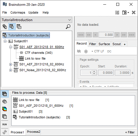
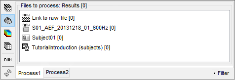
- The buttons on the left side allow you to select what type of file you want to process: Recordings, sources, time-frequency, other. When you select another button, all the counts are updated to reflect the number of files of the selected type that are found for each node.
Right now, if you select another file type, it would show only "0" everywhere because there are no sources or time-frequency decompositions available in the database yet.
- To remove files from the Process1 list:
Select the nodes to remove (holding Shift or Ctrl key) and press the Delete key.
Right-click on the list > Clear list
Filter by name or comment
When you have lots of files in a folder, like multiple source reconstructions or time-frequency files for each trial, it is difficult to grab just the ones you are interested in. After selecting your folders in the Process1 box, you can refine the selection with the Filter search box at the bottom-right corner of the window.
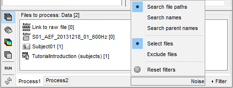
The example below shows how select the data file corresponding to the noise recordings: by typing "Noise" in the search box and selecting the option "Search file names". We cannot perform the search "by comment" because all the data files have the same comment "Link to raw file".
Reminder: To see the file name corresponding to a node in the database, leave your mouse over it for a few seconds. You can do this both in the database explorer and the Process1 list.

The options offered in the Filter menu are:
Search comments: Look for the string in the comments of the files, ie. what is displayed in the database explorer to represent them (the .Comment field).
Search file names: Look for the string in the full file names (including their relative path).
Select files: Only the files that contain the string are selected.
Exclude files: Only the files that DO NOT contain the string are selected.
Reset filters: Removes the current file filters applied on Process1 and Process2.
Case insensitive: Note that the search is not sensitive to case.
Selecting processes
- Clear the file list and the search filters.
- Select all the three datasets we have linked to our protocol. You can select the three "link to raw file" nodes, the three folders or the entire subject node.
Click on the [Run] button at the bottom-left corner of the Process1 tab.
The Pipeline editor window appears. You can use it to create an analysis pipeline, ie. a list of process that are applied on the selected files one after the other. The first button in the toolbar shows the list of processes that are currently available. If you click on a menu, it's added to the list.
- Some menus appear in grey. This means that they are not meant to be applied to the type of data that you have in input, or at the end of the current pipeline.
In the current example, we have a file with the type "continuous raw recordings", so we have access mostly to menus to manipulate event markers, run cleaning procedures and import data blocks. You can recognize a few operations that we execturd in the previous tutorials: "Event > Read from channel" and "Event > Detect analog triggers".
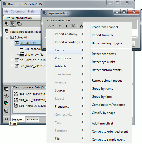
- When you select a process, a list of options specific to this process is shown in the window.
To delete a process: Select it and press the Delete key, or use the [X] button in the toolbar.
- After selecting a first process, you add another one. The output of the first process will be passed to the second process without giving back the control to the user. This is how you can build a full analysis pipeline with the interface.
- After adding a few processes, you can move up/down a process in the pipeline with the [up arrow] and [down arrow] buttons in the toolbar. Click on a process in the pipeline to edit its options.
- Select and delete a few processes to understand how this interface works. Just do not click on RUN.
Saving a pipeline
After preparing your analysis pipeline by listing all the operations to run on your input files, you can either click on the [Run] button, or save/export your pipeline. The last button in the the toolbar offers a list of menus to save, load and export the pipelines.
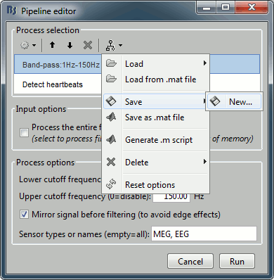
Load: List of processes that are saved in the user preferences
Load from file: Import a pipeline from a pipeline_...mat file (previously saved with the menu "Save as Matlab matrix")
Save: Save the pipeline in the user preferences, to be able to access it really fast after
Save as Matlab matrix: Exports the pipeline for a Matlab structure in a .mat file. Allows different users to exchange their analysis pipelines (or a single user between different computers).
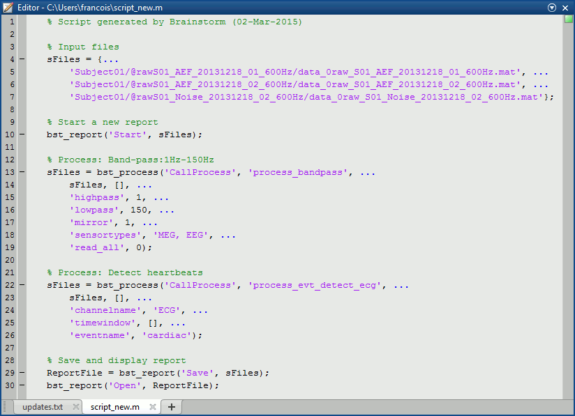
Generate .m script: This option generates a human-readable Matlab script that can be re-used for other purposes or modified.
Delete: Remove a pipeline that is saved in the user preferences.
Reset options: Brainstorm saves automatically for each user the options of all the processes. This menu removes all the saved options, and set them back to the default values.
Here is the Matlab script that is generated automatically for this pipeline.
Process: Select files with tag
You can get to the exact same result by adding the process "File > Select files with tag" before the process you want to execute, to keep only a subset of the files that were placed in the Process1 list. It is less convenient in interactive mode because you don't see immediately the effect of your file filter, but it can be very useful when writing scripts.
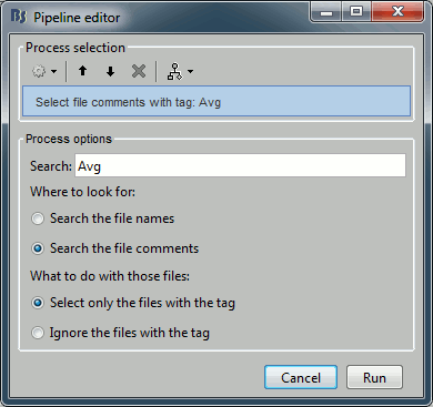
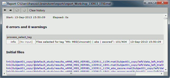
To see the list of files that was selected by the process, you can open the report viewer (File > Report viewer). This lists the input files (all the files) and the final files (the selected files), with a summary of how many files where selected on the top.
After
This process is useless if it is not followed immediately by another process that would do something with the selected files. An application can be the deletion of some files, by adding the process "File > Delete files".
How to control the output file names
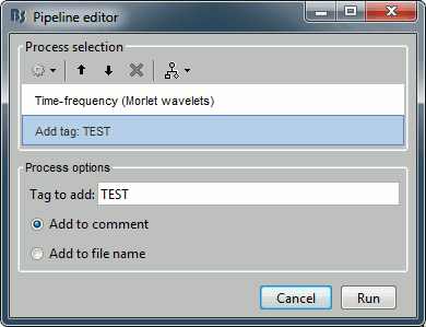
If you are running two processes with different parameters but that produce exactly the same file names and file comments, you wouldn't be able to select them with this process. But immediately after calling any process, you can add the process "File > Add tag" to tag one specific set of files, so that you can re-select them easily later.
Example: you run twice the time-frequency decomposition with different options on the same files, tag the files after calculating them with different tags.
Report viewer
Each time the pipeline editor is used to executed to run a list of processes, a report is generated and saved in the user home folder (/home/username/reports/). The report viewer shows as an HTML page some of the information saved in this report structure: the date and duration of execution, the list of processes, the input and output files. It reports all the warning and errors that happen during the execution.
The report viewer does not necessarily appear automatically at the end of the last process: it is shown only when more than one processes were executed, or when any of the processes returned an error or a warning.
When running processes manually from a script, the calls bst_report(Start, Save, Open) explicitly indicate when the logging of the events should start and stop.
You can add images to the reports for quality control using the process "File > Save snapshot".
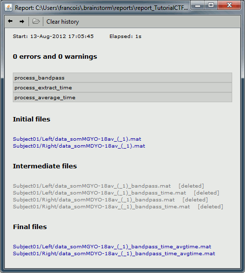
After you close the report window, you can re-open the last report with the main menu of the Brainstorm window: File > Report viewer.
With the buttons in the toolbar, you can go back to the previous reports saved from the same protocol.
PROCESSES AND PLUG-INS
The available processes are organized in a plug-in structure. Any Matlab script that is added to the plug-in folder (brainstorm3/toolbox/process/functions/) and has the right format will be automatically detected and made available in the GUI. This mechanism makes the contribution from other developers to Brainstorm very easy.
REPORT: OTHER TUTORIALS

