|
Size: 16533
Comment:
|
Size: 16534
Comment:
|
| Deletions are marked like this. | Additions are marked like this. |
| Line 84: | Line 84: |
| * Another faster solution, if you have access to digitized head shapes for all the subjects in the MEG files: skip the marking of the fiducials, use default positions estimated from MNI coordinates, and use the head shape for refining the registration. To force the BIDS importer to work this way, use the process "'''Import> Import anatomy > Import BIDS dataset'''" instead of the interactive menu, with the option "Align sensors using head points" selected. | * Another faster solution, if you have access to digitized head shapes for all the subjects in the MEG files: skip the marking of the fiducials, use default positions estimated from MNI coordinates, and use the head shape for refining the registration. To force the BIDS importer to work this way, use the process "'''Import > Import anatomy > Import BIDS dataset'''" instead of the interactive menu, with the option "Align sensors using head points" selected. |
Resting state recordings from the OMEGA database (2016)
Authors: Francois Tadel, Guiomar Niso, Elizabeth Bock, Sylvain Baillet
This tutorial introduces how to download resting state recordings from the OMEGA database and process them into Brainstorm. The goal is to evaluate where in the brain is distributed the power in specific frequency bands at rest. This example includes only 5 healthy subjects, but the same pipeline can be applied over larger populations.
Note that the operations used here are not detailed, the goal of this tutorial is not to introduce Brainstorm to new users. For in-depth explanations of the interface and theoretical foundations, please refer to the introduction tutorials.
Contents
OMEGA database
The Open MEG Archive (OMEGA) is the fruit of a collaborative effort by the McConnell Brain Imaging Centre and the Université de Montréal to build a centralized repository in which to regroup MEG data for open dissemination. This continuously expanding repository also contains anatomical MRI volumes, demographic and questionnaire information, and eventually will feature other forms of electrophysiological data (e.g. EEG, field, and cell recordings). OMEGA features the technological framework for multi-centric data aggregation, and is amongst the largest freely available resting-state MEG datasets presently available. Website: https://www.mcgill.ca/bic/resources/omega
You are free to use all data in OMEGA for research purposes; however, we ask that you please cite the following reference in your publications if you have used data from OMEGA:
Niso G, Rogers C, Moreau JT, Chen LY, Madjar C, Das S, Bock E, Tadel F, Evans A, Jolicoeur P, Baillet S
OMEGA: The Open MEG Archive, Neuroimage, 2015.
Presentation of the experiment
Experiment
- 5 subjects x 5 minute resting sessions, eyes open
MEG acquisition
Acquisition at 2400Hz, with a CTF 275 MEG system,
- Recorded at the Montreal Neurological Institute in 2015-2016.
- Anti-aliasing low-pass filter at 600Hz
- Files may be saved with or without the CTF 3rd order gradient compensation applied.
- Recorded channels (at least 297):
- 26 MEG reference sensors (#2-#27)
- 270 MEG axial gradiometers (#28-#297)
- 1 ECG bipolar (EEG057/#298) - Not available in the empty room recordings
- 1 vertical EOG bipolar (EEG058/#299) - Not available in the empty room recordings
- 1 horizontal EOG bipolar (EEG059/#300) - Not available in the empty room recordings
The data in this dataset has been organized according to the BIDS specifications
(Brain Imaging Data Structure, http://bids.neuroimaging.io)
Head shape and fiducial points
3D digitization using a Polhemus Fastrak device driven by Brainstorm. The .pos files contain:
- The center of the CTF coils,
The anatomical references we use in Brainstorm: nasion and ears as illustrated here,
- Around 100 head points distributed on the hard parts of the head (no soft tissues).
Subject anatomy
- Structural T1 image (defaced for anonymization purposes)
Processed with FreeSurfer 5.3
- The anatomical fiducials (NAS, LPA, RPA) have already been marked and saved in the files fiducials.m
Download and installation
First, make sure you have at least 40Gb of free space on your hard drive (raw files: 12Gb).
- The OMEGA database is not in it its final release stage, so we temporarily distribute the 5 subjects used in this tutorial from the Brainstorm website.
Go to the Download page, and download the file: sample_omega.zip
- Unzip it in a folder that is not in any of the Brainstorm folders (program folder or database folder).
Start Brainstorm (Matlab scripts or stand-alone version). For help, see the Installation page.
Select the menu File > Create new protocol. Name it "TutorialOmega" and select the options:
"No, use individual anatomy",
"No, use one channel file per condition".
BIDS specifications
The Brain Imaging Data Structure (BIDS) standard for neuroimaging data organization was first established for MRI and fMRI (Gorgolewski, 2016). It is based on simple file formats and folder structures that can readily expand to additional data modalities.
An extension of the BIDS for MEG datasets is currently under review. The data distributed with this tutorial is organized following this prototype (which may change in the future). One objective is that analysis pipelines designed with major analysis tools (such as Brainstorm, FieldTrip, MNE, SPM and others) can be readily applied without requiring software or pipeline redevelopments.
We have already implemented a set of functions that can load automatically into a Brainstorm database any dataset following the BIDS specification. The files that are read by this function are the following:
sample_omega/
derivatives/: Everything that cannot be considered as raw data
freesurfer/: Result of the FreeSurfer segmentation for all the subjects
sub-000X_ses-0001/: Output of FreeSurfer for subject 000X (session 0001)
sub-000X/: Raw data for subject 000X
ses-0001/: Only one session per subject (the subject visited the center only once)
anat/: Anatomical MRI scans for subject 000X (not used if FreeSurfer output available)
sub-000X_T1w.nii.gz: T1 scan
meg/: Unprocessed MEG recordings
sub-000X_task-rest_run-01_meg.ds: Resting MEG recordings (subject data)
sub-000X_task-noise_run-01_meg.ds: Empty room recordings (noise measure)
Import the dataset
Select the menu File > Load protocol > Import BIDS dataset > Select the folder sample_omega.
Keep the default values for all the questions that may be asked during the import process (eg. number of vertices in the cortex surfaces). Once done, you should be able to access the data for the 5 subjects in your database explorer: anatomy, and subject and noise recordings.
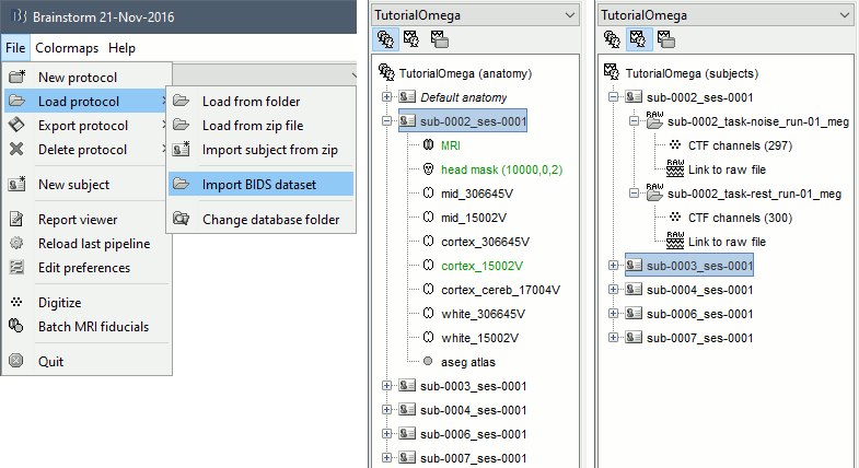
For this example dataset, the fiducials NAS/LPA/RPA were previously marked using the menu File > Batch MRI fiducials, which creates a file fiducials.m in the FreeSurfer folder. When importing the FreeSurfer folders, these fiducials are used by default.
- If you want to use this feature on your own BIDS-formatted dataset, using the menu Import BIDS dataset may ask you to select for each subject the position of the fiducials NAS/LPA/RPA. You can mark them in advance using the menu Batch MRI fiducials as we did.
Another faster solution, if you have access to digitized head shapes for all the subjects in the MEG files: skip the marking of the fiducials, use default positions estimated from MNI coordinates, and use the head shape for refining the registration. To force the BIDS importer to work this way, use the process "Import > Import anatomy > Import BIDS dataset" instead of the interactive menu, with the option "Align sensors using head points" selected.
Pre-processing
- Switch to the functional view of the protocol (second button above the database explorer).
- Drag and drop all the subjects into the Process1 box, and click on [Run].
Select process: Import > Import recordings > Convert to continuous: Continuous
Add process: Frequency > Power spectrum density (Welch): All file, 4s, 50% overlap, Individual
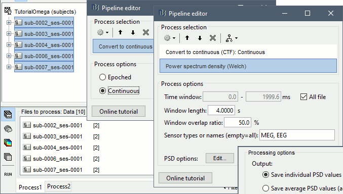
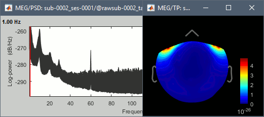
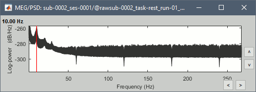
Run, then check the quality of the PSD for all the files, as documented in this tutorial.
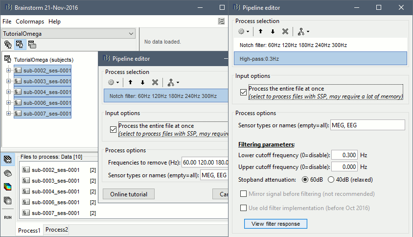
- In Process1, keep the same files selected and click on [Run].
Select process: Pre-process > Notch filter: 60 120 180 240 300 Hz, Process the entire file at once
Add process: Pre-process > Band-pass filter: High-pass filter at 0.3Hz, 60dB, Process entire file.
Add process: Frequency > Power spectrum density (Welch): Same options
Run, then check the PSD after filtering.
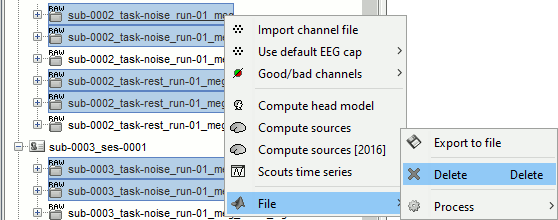
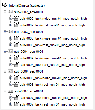
Delete all the folders corresponding to the original recordings (_meg) and the notch filtered data (_meg_notch). Only keep the fully processed files (_meg_notch_high).
Artifact cleaning
We will now run the automatic procedure for cleaning the heartbeats, as described in the introduction tutorials (detection, SSP). The results we want to illustrate here are robust enough, the recordings do not need to be processed any further. If you want to improve the quality of the data with more manual cleaning (blinks, saccades, movements, bad segments), please refer to the introduction tutorials.
In Process1, select all the subject rest recordings (task-rest).
Select process: Events > Detect heartbeats: ECG, All file, cardiac
Add process: Artifacts > SSP: Heartbeats: cardiac, MEG, Use existing SSP
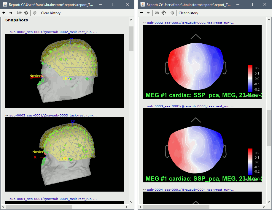
Add process: File > Snapshot: Sensor/MRI registration
Add process: File > Snapshot: SSP projectors
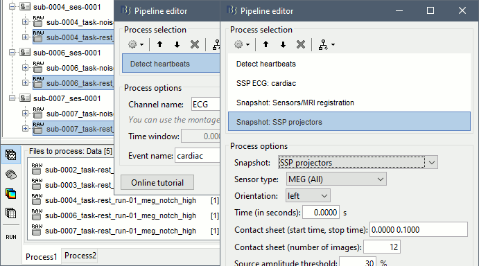
Run, then review the registration and the SSP topographies for all the subjects. Make sure that the subjects' heads are well aligned in the MEG, and that the spatial components that are removed are really representative of the cardiac artifact.
Source estimation
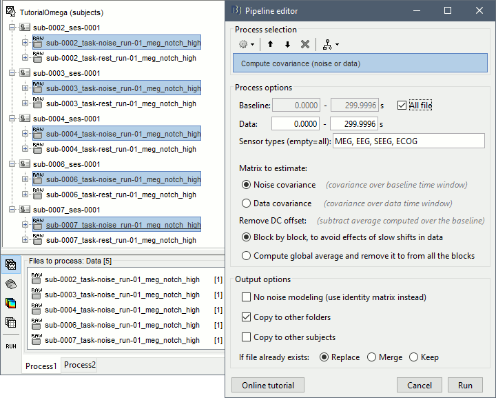
In Process1, select all the noise recordings (task-noise).
Run process: Sources > Compute covariance: All file, Noise covariance, Copy to other folders.
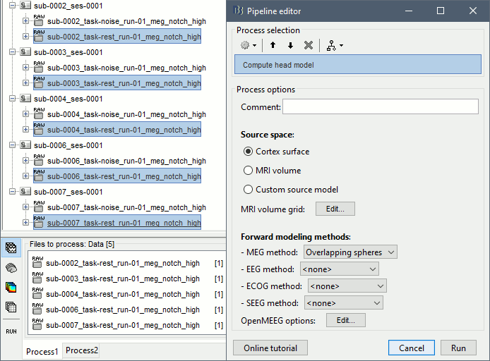
In Process1, select all the subject rest recordings (task-rest).
Run process: Sources > Compute head model: Cortex surface, MEG=Overlapping spheres.
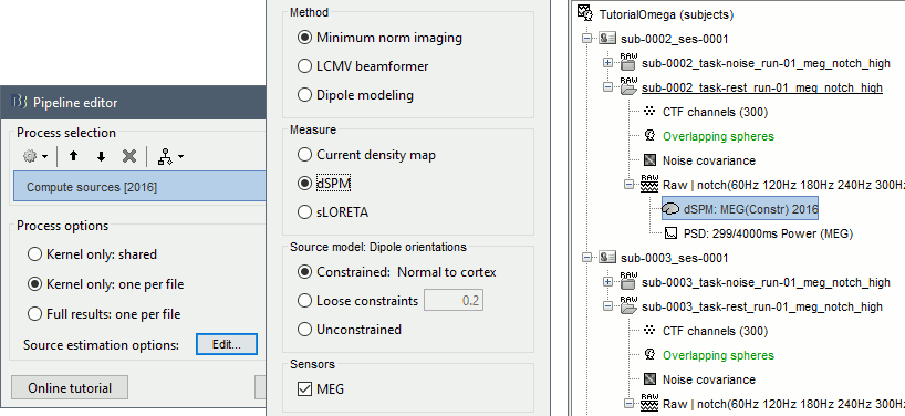
Run process: Sources > Compute sources [2016]: Kernel only, one per file, dSPM, constrained.
Power maps
We have now access to continuous recordings in source space, we can estimate the average power over this resting period, for various frequency bands. We propose here to compute the PSD from the first 100s instead of the full 600s rest recordings, it is faster and leads to very similar results. For more stable estimates, you can compute the the PSD over all the data available instead.
In Process1, select all the subject rest recordings (task-rest), click the [Process sources] button.
Select process: Frequency > Power spectrum density (Welch): [0,100s], Window=4s, 50% overlap, Group in frequency bands (use the default frequency bands), Save individual PSD values.
Add process: Standardize > Spectrum normalization: Relative power (divide by total power). This normalization is done independently for each source, the output for each frequency band is a percentage of how much this frequency band contributes to the total power of the source signal.
Add process: Sources > Project on default anatomy: Cortex.
Add process: Sources > Spatial smoothing: FWHM=3mm, Overwrite.
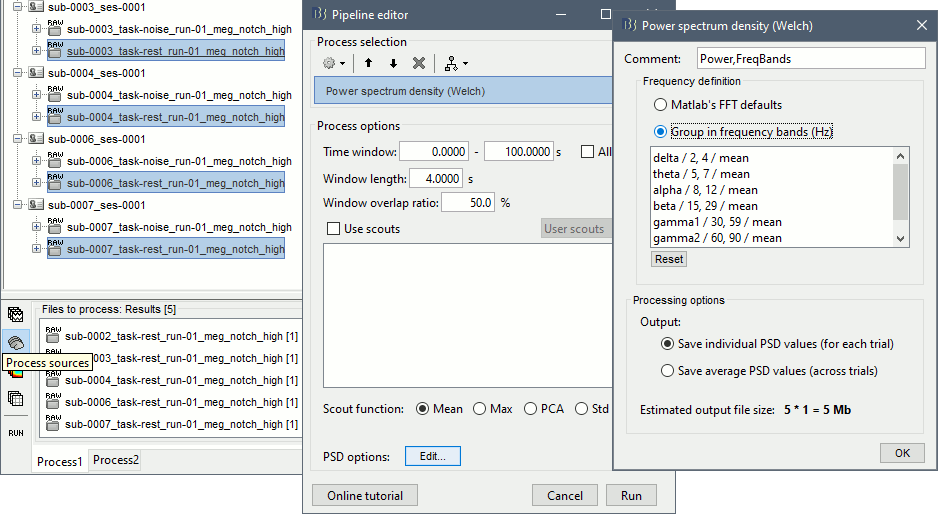
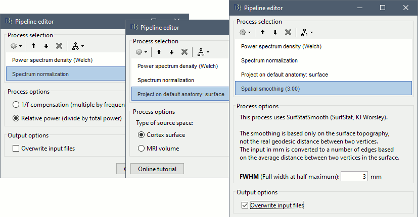
- Execute this pipeline, then open the results for the different subjects and visualize the different frequency bands. They should look similar across subjects. This measure of relative power is very robust and usually do not vary much between subjects or duration of the input signals.
The values in this figure represent the relative power of each source. At each vertex of the cortex surface, the value between 0 and 1 indicates what is the contribution of the current frequency band to the total power in the signal. To obtain comparable colormaps across multiple figures, you can set a fixed maximum (right-click on a figure > Colormap: Timefreq > Maximum: Custom).
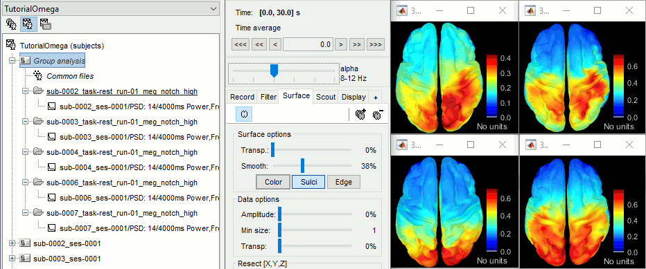
We will now average these files across subjects. In Process1, select all the projected subject averages in the Group analysis folder, and click on the button [Process time-freq].
Run process: Average > Average files: Everything, Arithmetic average, Do not match signals
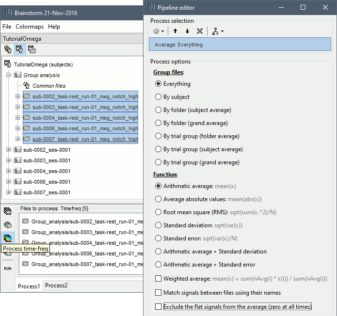
Double-click on the average to display it. To create the figures below, right-click on the figure > Snapshot > Frequency contact sheet.
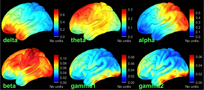
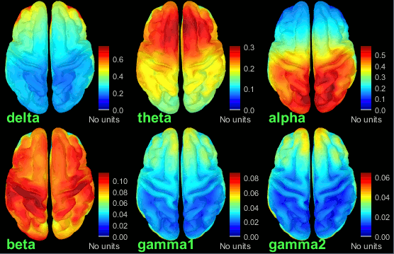
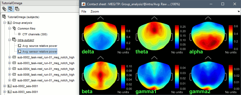
- We can relate these figures with associations commonly reported in the literature:
Theta: Mostly frontal.
Alpha: Parieto-occipital.
Beta: Central regions (motor cortex).
Gamma: Pre-frontal and occipital. However, the occipital sources could be related with muscle activity in the neck. We haven't cleaned the recordings much, we should go back to the recordings and mark as bad all the segments in which we observe a lot of muscle activity.
Delta: Questionable - these source maps showing high values at the poles of the frontal and temporal lobes are typical of eye movements. We should try doing some cleaning of the ocular artifacts (blinks and saccades) and compute these maps again.
You can compute the same results in the head volume. You just have to use a volume head model on a group grid instead of the one we used here. This is explained in the tutorial Group analysis. This seems to confirm that the power in the delta and gamma bands is mostly coming from non-brain regions (eyes and neck muscles).
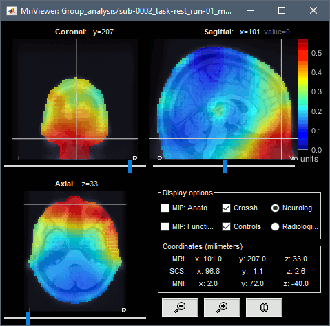
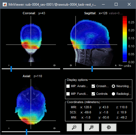
You can produce similar plots at the sensor level: Compute the PSD by frequency band of the rest recordings for each subject, then compute the average across subjects (not as reliable as averaging in source space, as explained here).
Resting state metrics [TODO]
Discuss what other measures can be used in resting state MEG.
Add references to a few recent publications.
Scripting
The following script from the Brainstorm distribution reproduces the analysis presented in this tutorial page: brainstorm3/toolbox/script/tutorial_omega.m
