|
Size: 13533
Comment:
|
Size: 12239
Comment:
|
| Deletions are marked like this. | Additions are marked like this. |
| Line 7: | Line 7: |
| * Let's look at the first file in the list: AEF#01 * Right-click on the Link to raw file. Below the first to menus, you have the list of channel types: * '''MEG''': 274 axial gradiometers * '''ECG''': 1 electrocadiogram, bipolar electrode across the chest * '''EOG''': 2 electrooculograms (vertical and horizontal) * '''Misc''': EEG electrodes Cz and Pz * '''ADC A''': Unused * '''ADC V''': Auditory signal sent to the subject * '''DAC''': Unused * '''FitErr''': Fitting error when trying to localize the three head localization coils (NAS, LPA, RPA) * '''HLU''': Head Localizing Unit, displacements in the three directions (x,y,z) for the three coils * '''MEG REF''': 26 reference sensors used for removing the environmental noise * '''Other''': Unused * '''Stim''': Stimulation channel, records the stim triggers generated by the Psychophysics toolbox * '''SysClock''': System clock, unused * Select > MEG > Display time series (or double-click on the file).<<BR>><<BR>> {{attachment:link_menu.gif||height="322",width="324"}} * It will open a new figure and enable many controls in the Brainstorm window.<<BR>><<BR>> {{attachment:review_epoch.gif}} |
Let's look at the first file in the list: AEF#01.<<BR>>Right-click on the Link to raw file. Below the first to menus, you have the list of channel types: * '''MEG''': 274 axial gradiometers * '''ECG''': 1 electrocadiogram, bipolar electrode across the chest * '''EOG''': 2 electrooculograms (vertical and horizontal) * '''Misc''': EEG electrodes Cz and Pz * '''ADC A''': Unused * '''ADC V''': Auditory signal sent to the subject * '''DAC''': Unused * '''FitErr''': Fitting error when trying to localize the three head localization coils (NAS, LPA, RPA) * '''HLU''': Head Localizing Unit, displacements in the three directions (x,y,z) for the three coils * '''MEG REF''': 26 reference sensors used for removing the environmental noise * '''Other''': Unused * '''Stim''': Stimulation channel, records the stim triggers generated by the Psychophysics toolbox * '''SysClock''': System clock, unused Select > MEG > Display time series (or double-click on the file). . {{attachment:link_menu.gif||height="322",width="324"}} It will open a new figure and enable many controls in the Brainstorm window. . {{attachment:review_epoch.gif}} |
| Line 29: | Line 35: |
| * '''Click''': Click on the white parts of figure to move the time cursor (red vertical line).<<BR>>If you click on the signals, it will select the corresponding channels, click again to unselect. | * '''Click''': Click on the white or grey parts of figure to move the time cursor (red vertical line).<<BR>>If you click on the signals, it selects the corresponding channels. Click again to unselect. |
| Line 32: | Line 38: |
| * '''Zoom''': Scroll to zoom horizontally around the time cursor (mouse wheel or two-finger up/down). | |
| Line 47: | Line 54: |
| '''Time selection''' |
==== Time selection ==== |
| Line 61: | Line 67: |
| * Increase the duration of the displayed window to '''3 seconds''' (Page settings > Duration). <<BR>><<BR>> {{attachment:review_continuous.gif}} | * Increase the duration of the displayed window to '''3 seconds''' (Page settings > Duration). <<BR>><<BR>> {{attachment:review_continuous.gif||height="191",width="561"}} |
| Line 64: | Line 70: |
| * '''AEF#02''' > Switch epoched/continuous * '''Noise''' > Switch epoched/continuous |
* '''AEF#02 > Switch epoched/continuous ''' * '''Noise''' '''> Switch epoched/continuous ''' == Display mode: Butterfly/Column == * Close all the figures. * Double-click on the AEF#01 Link to raw file to open the MEG recordings. * What we see are all the traces of the 274 sensors overlaid on top of each other. * Click on the "Display mode" button in the toolbar of the Record tab. <<BR>><<BR>> {{attachment:review_switch.gif}} * All the signals are now displayed one below the other, but because we have 274 MEG channels, the figure is still unreadable. We need to select only a subset of those sensors. <<BR>><<BR>> {{attachment:review_column.jpg||height="186",width="381"}} == Montage selection == * You can use the montage menu to select a group of sensors. This menu is accessible in two ways: * Record toolbar > Drop-down menu. * Figure popup menu > Right-click on the figure > Montage * Pre-defined groups of channels are available for some common MEG and EEG systems.<<BR>>Notice the keyboard shortcuts on the right (Shift+A, B, C...). * You can also use this menu to create your own sensor selections or more complex montages.<<BR>>A separate tutorial is dedicated to the montage editor. * Select the group: '''CTF LT''' (Left Temporal, Shift+D). <<BR>><<BR>> {{attachment:review_montage.gif||height="190",width="527"}} |
| Line 68: | Line 89: |
| If you click on the lines instead of the white area: select channels. | If you click on the white or grey areas of the figure, it changes the current time. <<BR>>If you click on the lines representing the recorded signals instead, it selects the corresponding channels. |
| Line 70: | Line 91: |
| == Montage selection == Let's switch to a nicer representation of the recordings time series: click on the "Display mode" button in the toolbar of the Record tab. {{http://neuroimage.usc.edu/brainstorm/Tutorials/TutRawViewer?action=AttachFile&do=get&target=tsColumn.gif|tsColumn.gif|class="attachment"}} Now the traces are displayed in columns, but all the channels are displayed in the same figure, which makes it unreadable. Select a subset of channels by right-clicking on the figure > '''Montages''', with the drop-down menu in the Record tab or with a keyboard shortcut ('''Shift+A, B, C'''...). Default groups of sensors are available for some MEG systems, but you can also create your own groups of sensors with the menu "Edit montages". The montage editor is described in the next tutorial. {{http://neuroimage.usc.edu/brainstorm/Tutorials/TutRawViewer?action=AttachFile&do=get&target=tsChannelSelection.gif|tsChannelSelection.gif|class="attachment"}} |
* When some channels are selected, an additional menu "Channels" is visible in the figure popup. * Select "View selected" or press [Enter] to open the selected channels in a separate window. * If you select channels in one figure, this selection will always be applied to all the other figures. * The management of the bad channels will be introduced in a separate tutorial.<<BR>><<BR>> {{attachment:channel_select.gif||height="246",width="615"}} |
| Line 80: | Line 97: |
| In this display mode, the amplitude scale is represented on the right of the figure. You can adjust this vertical scale: | A variety of display options allows you to adjust the amplitude scale for the recordings (vertical axis). |
| Line 82: | Line 99: |
| * Use the buttons "'''^'''" and "'''v'''" on the right side of the figure. The shortcuts for those buttons are indicated in the tooltips (leave the mouse for a short while over a button) * Hold the '''Shift key''' and move the mouse wheel, or use the keys "'''+'''" and "'''-'''". * Use the button "'''...'''" on the right side of the figure ("Set scale manually") to set the scale to a precise level. |
. {{attachment:review_scale.gif}} |
| Line 86: | Line 101: |
| When scrolling in time to a different page, the amplitude scale is by default kept. You can change this behavior to re-evaluate automatically an optimal scale each time you change the current time window. This option is called "Auto-scale amplitude" and is disabled by default. To activate it: click on the "'''AS'''" button on the right of the figure, or check the menu "'''Display > Auto-scale amplitude'''" in the Record tab. | * '''Increase/decrease gain''': Buttons '''[^]''' and '''[v]''' on the right side of the figure. The shortcuts for those buttons are indicated in the tooltips (leave the mouse for a short while over a button).<<BR>>Hold the '''Shift key''' and scroll, or use the keys '''[+]''' and '''[-]'''. * '''Flip +/-''': Button in the right part of the time series figure. Exchange the direction of the Y axis, to have the peaks of negative values pointing up. Useful mostly for clinical EEG. * '''Set scale manually''': Button '''[...]''' in the figure. Forces a defined amplitude scaling. * '''Auto-scale amplitude''': Button '''[AS]''' in the figure. <<BR>>Selected: the vertical scale is adapted to the new maximum amplitude when you scroll in the file. <<BR>>Not selected: The vertical scale is fixed, scrolling in the file does not affect the display. |
| Line 88: | Line 106: |
| == Display options == . {{http://neuroimage.usc.edu/brainstorm/Tutorials/TutRawViewer?action=AttachFile&do=get&target=displayOptions.gif|displayOptions.gif|class="attachment"}} |
* '''Remove DC offset''': Button '''[DC]''' in the Record tab. When selected, the average value over the entire current time window is subtracted from each channel. This means that if you change the length of the time window, the value that is removed from each channel may change. Always keep this option selected for unprocessed MEG recordings, unless you use a high-pass filter. |
| Line 91: | Line 108: |
| * '''Remove DC offset''': Button [DC] in the Record tab. When selected, for each channel, the average value over the entire current time window is subtracted from the channel values. This means that if you change the length of the time window, the value that is removed from each channel may change. It doesn't make much sense to disable this option for unprocessed MEG recordings. * '''Apply CTF compensation''': Button [CTF] in the Record tab. Enable/disable the CTF noise correction based on the reference sensors, when it is not already applied in the file. In the current file, the CTF 3rd order gradient compensation is already applied, therefore this option is not available. * '''Flip +/-''': Button in the right part of the time series figure. Exchange the direction of the Y axis, useful mostly for clinical EEG. * '''Set scale manually''': Button [...] in the figure. Forces a defined amplitude scaling. * '''Auto-scale amplitude''': Button [AS] in the figure. When selected, the vertical scale is adapted to the maximum value over the time window when the time window changes. When not selected: the vertical scales keeps its last value when you jump to another part of the file. |
* '''Apply CTF compensation''': Button [CTF] in the Record tab. Enable/disable the CTF noise correction based on the reference sensors, when it is not already applied in the file. In the current file, the CTF 3rd order gradient compensation is already applied, therefore this option is not available. |
| Line 99: | Line 111: |
| With the Filter tab, you can apply a band-pass filter to the recordings, or remove a set of specific frequencies (example: the 50Hz or 60Hz power lines contamination and their harmonics). The filters are applied only to the time window that is currently loaded; hence if the segment is too short for the required filters, the results could be inaccurate. | With the Filter tab, you can apply a band-pass filter to the recordings, or remove a set of specific frequencies (example: the 50Hz or 60Hz power lines contamination and their harmonics). The filters are applied only to the time window that is currently loaded. If the segment is too short for the required filters, the results might be inaccurate. |
| Line 105: | Line 117: |
| {{http://neuroimage.usc.edu/brainstorm/Tutorials/TutRawViewer?action=AttachFile&do=get&target=onlineFilter.gif|onlineFilter.gif|class="attachment"}} | {{attachment:review_filter.gif}} |
| Line 140: | Line 152: |
| = From CTF = == Time selection == Go back to the previous view mode ("butterfly view") and in the Record tab, select the menu "All channels" again. Keep this selection for the rest of the tutorial. * Left-click somewhere on the white part of the time series figure, hold the mouse button, and drag your mouse left or right: A transparent blue rectangle appears to represent the time selection. * Now right-click on the figure to see the functions you can apply on this time window. The selected time window and its duration are shown at the bottom of the figure. . {{http://neuroimage.usc.edu/brainstorm/Tutorials/TutExploreRecodings?action=AttachFile&do=get&target=timeSelection.gif|timeSelection.gif|class="attachment"}} * '''Set current time''': Just sets the time cursor when the right-click occurred. The shortcut Shift+Click can be useful when trying to move in time on dense displays in columns view. * '''Set selection manually''': Select a time window by giving the bounds in ms. * '''Average over time''': Average over the selected time window, saved as a new file in the database. * '''Export to database''': Extract the recordings and save them in a new file in database. * If some sensors are selected, only their values are extracted, all the others are set to zero. * '''Export to file''': Same, but in a user-defined file (not in the database) * '''Export to Matlab''': Same, but export as a Matlab variable in the current workspace. |
Tutorial 5: Review continuous recordings
Authors: Francois Tadel, Elizabeth Bock, John C Mosher, Sylvain Baillet
Contents
Open the recordings
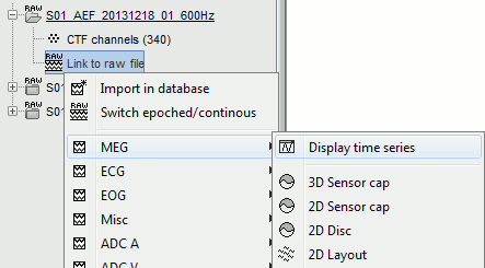
Let's look at the first file in the list: AEF#01.
Right-click on the Link to raw file. Below the first to menus, you have the list of channel types:
MEG: 274 axial gradiometers
ECG: 1 electrocadiogram, bipolar electrode across the chest
EOG: 2 electrooculograms (vertical and horizontal)
Misc: EEG electrodes Cz and Pz
ADC A: Unused
ADC V: Auditory signal sent to the subject
DAC: Unused
FitErr: Fitting error when trying to localize the three head localization coils (NAS, LPA, RPA)
HLU: Head Localizing Unit, displacements in the three directions (x,y,z) for the three coils
MEG REF: 26 reference sensors used for removing the environmental noise
Other: Unused
Stim: Stimulation channel, records the stim triggers generated by the Psychophysics toolbox
SysClock: System clock, unused
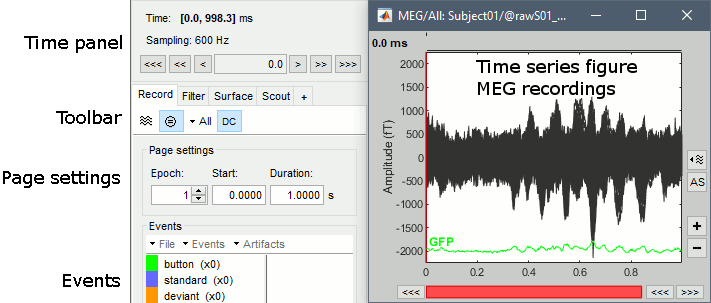
Select > MEG > Display time series (or double-click on the file).
It will open a new figure and enable many controls in the Brainstorm window.
Navigate in time
The files we have imported here are shown the way they have been saved by the CTF MEG system: as contiguous epochs of 1 second each. Those epochs are not related with the stimulus triggers or the subject's responses, they are just a way of saving the files. We will first explore the recordings in this epoched mode before switching to the continuous mode.
From the time series figure
Click: Click on the white or grey parts of figure to move the time cursor (red vertical line).
If you click on the signals, it selects the corresponding channels. Click again to unselect.Shortcuts: See the tooltips in the time panel for important keyboard shortcuts:
Left arrow, right arrow, page up, page down, F3, Shift+F3, etc...Bottom bar: The red square in the bottom bar represents the portion of the file that is currently displayed from the current file or epoch. Right now we show all the epoch #1. This will be more useful in the continuous more.
Zoom: Scroll to zoom horizontally around the time cursor (mouse wheel or two-finger up/down).
[<<<] and [>>>]: Previous/next epoch or page
From the time panel
Time: [0, 998]ms is the time segment over which the first epoch is defined.
Sampling: We downsampled these files to 600Hz for easier processing in the tutorials.
Text box: Current time, can be edited manually.
[<] and [>]: Previous/next time sample - Read the tooltip for details and shortcuts
[<<] and [>>]: Previous/next time sample (x10) - Read the tooltip for details and shortcuts
[<<<] and [>>>]: Previous/next epoch or page - Read the tooltip for details and shortcuts
From the page settings
Epoch: Selects the current time block that is displayed in the time series figure.
Start: Starting point of the time segment displayed in the figure. Useful is continuous mode only.
Duration: Length of this time segment. Useful is continuous mode only.
Time selection
- In the time series figure, click and drag your mouse for selecting a time segment.
- At the bottom of the figure, you will see the duration of the selected block.
- Useful for quickly estimating the latencies between two events, or the period of an oscillation.
Click anywhere on the figure to cancel this time selection.

Epoched vs. continuous
- The CTF MEG system can save two types of files: epoched (.ds) or continuous (_AUX.ds).
- Here we have an intermediate storage type: continuous recordings saved in "epoched" files. The files are saved as small blocks of recordings of a constant time length (1 second in this case). All those time blocks are contiguous, there is no gap between them.
- Brainstorm can consider this file either as a continuous or an epoched file. By default it imports the regular .ds folders as epoched, but we can change this manually, to process it as a continuous file.
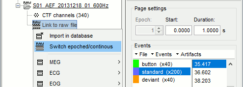
Right-click on the "Link to raw file" for AEF#01 > Switch epoched/continuous
You should get a message: "File converted to: continuous".- Double-click on the "Link to raw file" again. Now you can navigate in the file without interruptions. The box "Epoch" is disabled and all the events in the file are displayed at once.
Increase the duration of the displayed window to 3 seconds (Page settings > Duration).
- Close the figure.
- Repeat this operation with the other files to convert them all to a continuous mode.
AEF#02 > Switch epoched/continuous
Noise > Switch epoched/continuous
Display mode: Butterfly/Column
- Close all the figures.
- Double-click on the AEF#01 Link to raw file to open the MEG recordings.
- What we see are all the traces of the 274 sensors overlaid on top of each other.
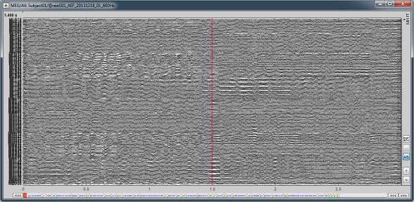
Click on the "Display mode" button in the toolbar of the Record tab.

All the signals are now displayed one below the other, but because we have 274 MEG channels, the figure is still unreadable. We need to select only a subset of those sensors.
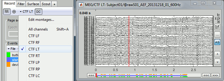
Montage selection
- You can use the montage menu to select a group of sensors. This menu is accessible in two ways:
Record toolbar > Drop-down menu.
Figure popup menu > Right-click on the figure > Montage
Pre-defined groups of channels are available for some common MEG and EEG systems.
Notice the keyboard shortcuts on the right (Shift+A, B, C...).You can also use this menu to create your own sensor selections or more complex montages.
A separate tutorial is dedicated to the montage editor.Select the group: CTF LT (Left Temporal, Shift+D).
Channel selection
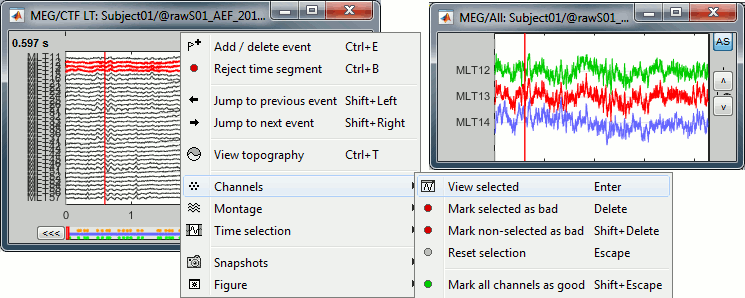
If you click on the white or grey areas of the figure, it changes the current time.
If you click on the lines representing the recorded signals instead, it selects the corresponding channels.
- When some channels are selected, an additional menu "Channels" is visible in the figure popup.
- Select "View selected" or press [Enter] to open the selected channels in a separate window.
- If you select channels in one figure, this selection will always be applied to all the other figures.
The management of the bad channels will be introduced in a separate tutorial.
Amplitude scale
A variety of display options allows you to adjust the amplitude scale for the recordings (vertical axis).
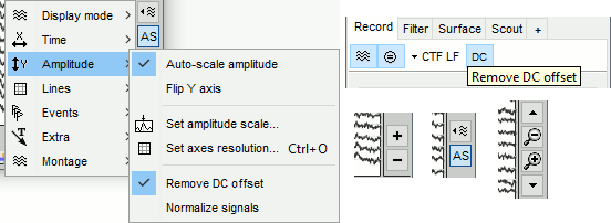
Increase/decrease gain: Buttons [^] and [v] on the right side of the figure. The shortcuts for those buttons are indicated in the tooltips (leave the mouse for a short while over a button).
Hold the Shift key and scroll, or use the keys [+] and [-].Flip +/-: Button in the right part of the time series figure. Exchange the direction of the Y axis, to have the peaks of negative values pointing up. Useful mostly for clinical EEG.
Set scale manually: Button [...] in the figure. Forces a defined amplitude scaling.
Auto-scale amplitude: Button [AS] in the figure.
Selected: the vertical scale is adapted to the new maximum amplitude when you scroll in the file.
Not selected: The vertical scale is fixed, scrolling in the file does not affect the display.Remove DC offset: Button [DC] in the Record tab. When selected, the average value over the entire current time window is subtracted from each channel. This means that if you change the length of the time window, the value that is removed from each channel may change. Always keep this option selected for unprocessed MEG recordings, unless you use a high-pass filter.
Apply CTF compensation: Button [CTF] in the Record tab. Enable/disable the CTF noise correction based on the reference sensors, when it is not already applied in the file. In the current file, the CTF 3rd order gradient compensation is already applied, therefore this option is not available.
Online filter
With the Filter tab, you can apply a band-pass filter to the recordings, or remove a set of specific frequencies (example: the 50Hz or 60Hz power lines contamination and their harmonics). The filters are applied only to the time window that is currently loaded. If the segment is too short for the required filters, the results might be inaccurate.
The option "Mirror signal before filtering" triples artificially the length of the signal with a mirror symmetry on each side, to avoid the strong edge effects that those filters can generate. Those online filters are not very accurate, they just provide a quick estimate for visualization only, the results are not saved anywhere. To filter properly the continuous files, please use the Process1 tab.
After testing the high-pass, low-pass and notch filters, uncheck them. If not you will probably forget about them, and they will stay on until you restart Brainstorm.

Shortcut summary
Keyboard shortcuts
Left / right arrows:
- No other key: Change current time, sample by sample
With Control key: Jump to previous/next time segment (same as the "<<<" and ">>>" buttons)
With Shift key: Jump to next event of the selected group
On MacOS, these shortcuts are different: please read the tooltips from the buttons ">", ">>", and ">>>" in the time panel to get the appropriate shortcuts.
Page-up / page-down:
- Same as left/right arrows, but faster (10 samples at a time)
If epochs are defined in the file: Control + page-up/page-down jumps to the next/previous epoch.
F3/Shift+F3: Jump to the next/previous epoch or page
F4/Shift+F4: Jump to the next/previous half-page
Plus / minus: Adjust the vertical scale of the time series
Control + E: Add / delete event occurrence
Control + T: Open a 2D topography window at the current time
Shift + Letter: Changes the set of electrodes currently displayed in the figure (list available by right-clicking on the figure > Display setup > ...)
Enter: Display the selected channels in a separate figure (selected channels = lines on which you clicked, that are shown in red)
Escape: Unselect all the selected channels
Delete: Mark the selected channels as bad
Mouse shortcuts
Mouse click on a channel: Select the channel
Mouse click: Change current time
Mouse click + Shift: For the selection of the current time (do not select any sensor, even when clicking on a line)
Mouse click + move: Select time range
Mouse wheel: Zoom around current time
Control + mouse wheel: Zoom vertically
Shift + mouse wheel: Adjust the vertical scale of the time series
Right-click: Display popup menu
Right-click + move: Move in a zoomed figure
Double click: Restore initial zoom settings (but do not restore the vertical scale of the time series)

