Spectral Parameterization Resolved in Time (SPRiNT)
Author: Luc Wilson
This tutorial introduces the features developed in Brainstorm to compute and view SPRiNT models, or time-resolved parameterized spectral density maps.
Contents
Introduction
The Spectral Parameterization Resolved in Time (SPRiNT) algorithm is designed to identify and model spectral features of the neural activity across time. Beginning with the time-series, it performs a short-time Fourier transform (STFT) and averages windows locally in time to generate local-mean power spectra, before decomposing these spectra into aperiodic and periodic components using specparam. The present tutorial will demonstrate the algorithm’s functionality within the Brainstorm interface.

This demonstration uses sample data from the introduction dataset, and can be followed by completing all steps of the Brainstorm tutorial up to and including tutorial 10.
Note: SPRiNT uses the MATLAB implementation of specparam.
Preparing the data for SPRiNT
SPRiNT is performed on time series, so we will first prepare some data from our notch-filtered dataset.
- Right-click "Link to raw file" in the folder "S01_AEF_20131218_01_600Hz_notch"
Select Import to database. In this tutorial, we will use the data from 60-120 s.
If you haven't already, now is a good time to remove DC offset. This will not affect our analyses, but it makes it easier to visualize our data as a time-series.- Click on [Import] to import the dataset into the database. The imported data will be placed in a new folder at the bottom of the list.
Initializing and running SPRiNT
- Clear the list of files in the Process1 tab.
- Select "Raw (60.00s,120.00s)" from the newly created folder and add it to Process1.
- Click on [Run] to open the pipeline editor window.
Select the process "Frequency > SPRiNT: Spectral Parameterization Resolved in Time".
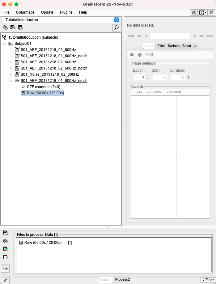
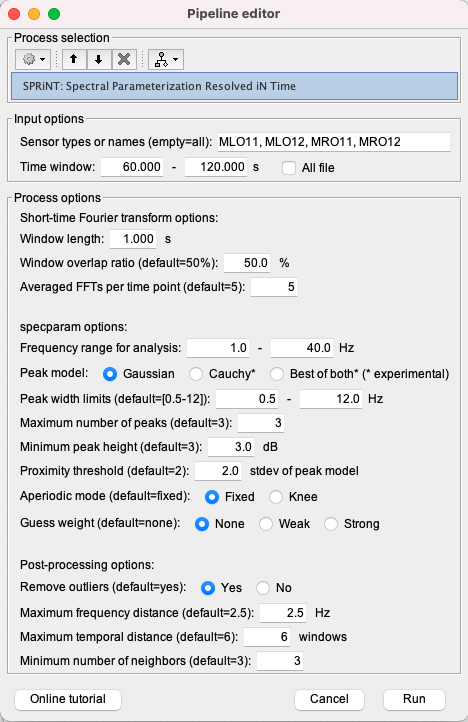
Select the following input options:
Sensor types or names (empty=all): MLO11, MLO12, MRO11, MRO12
This option allows you to choose which sensors you would like to run the process on. These four sensors were chosen for demonstration purposes, but any sensor will suffice.Time window: 60.00-120.00s
This option allows you to choose the time region you would like to run the process on.
Select the following process options:
Short-time Fourier transform options relate to how the STFT process is performed over the time-series.
Window length: 1.0 s.
This option changes the length of each window used in the short-time Fourier transform. Longer windows yield higher frequency resolutions (Frequency resolution = 1/window length).Window overlap ratio: 50% [default: 50%]
This option changes the degree to which each window used in the short-time Fourier transform overlaps.Averaged FFTs per time point: 5 [default: 5]
This option determines the number of short-time Fourier transform windows averaged locally at each time point. More windows tend to produce smoother spectra at the cost of temporal specificity. We recommend using odd numbers of windows, as this ensures the middle window in the center of the timepoint it represents.
Spectral parameterization options relate to how specparam parameterizes the resulting time-resolved spectra.
Frequency range for analysis: 1.0 - 40.0 Hz [default: 1.0 - 40.0 Hz].
specparam is best performed on a subset of the frequencies from the original PSD. In this range, it is important to avoid frequencies which have previously been filtered, as their adjusted powers can alter model results adversely.Peak model: Gaussian [default: Gaussian].
specparam fits spectral peaks using a gaussian distribution; Brainstorm also allows the algorithm to fit peaks using a Cauchy distribution (if desired) because SPRiNT uses the MATLAB implementation of specparam. The final option ("Best of Both") allows for individual timepoints to be fit using the function which minimizes model mean squared error (MSE).Peak width limits: 0.5 - 12.0 Hz [default: 0.5 - 12.0 Hz].
The bounds for putative peaks to be included in the SPRiNT maps. Putative peaks with widths estimated outside these bounds are discarded.Maximum number of peaks: 3 [default: 3].
The maximum number of attempts the model will make to identify peaks; it is best to allow for at least the number of clearly visible peaks in non-modelled time-frequency space plus one, in the event that the model does not remove a larger peak entirely in the peak-identification process.Minimum peak height: 3.0 dB [default: 3 dB].
The minimum peak height (in log[Power]) necessary for putative peaks to be included in the final SPRiNT maps. Putative peaks with heights estimated to be smaller than this threshold will be discarded.Proximity threshold: 2 standard deviations of the (comparatively) largest peak [default: 2].
Occasionally, the algorithm can mistake components of a single peak as two smaller peaks. This option forces the smaller of two peaks which are too close to one-another (i.e. If the center frequency of the smaller peak is within this value of standard deviations of the larger peak’s center frequency), the smaller of the two peaks is discarded. This option also removes peaks within this value of their standard deviation from the edge of the frequency window.Aperiodic mode: Fixed [default: Fixed].
The aperiodic component of the neural power spectrum occasionally presents with a knee, as seen below in log-log space. When selecting this option, you should first consult your data to determine whether it has a knee or not (Note: a knee component is present when the aperiodic features of the spectrum plotted in log-log space are not linear).Guess weight: Weak [default: None].
By design, peak parameter estimates are close to the actual fit. However, fitting a distribution that does not match the spectrum precisely (i.e. fitting a gaussian distribution to an imperfect gaussian-shaped peak) can occasionally lead to semantically worse-fit models; square error is reduced, but the model does not look as much like the data. Selecting this option allows for additional model error to be placed on parameter values which lie further from initial estimates. “Weak” represents a small penalty, while “Strong” represents a larger penalty (essentially keeping the pre-optimization estimates). When this option is set to “None”, the algorithm reduces square error most similarly to the Python version of specparam.Note: Guess weight selections are ignored when Brainstorm detects that the user has the optimization toolbox, as it will use constrained optimization to best-match the Python version of specparam. It is recommended that users have the optimization toolbox.
Post-processing options relate to if and how outlier peaks are removed following spectral parameterization.
Remove outliers: yes [default: yes]
This option toggles post-process outlier peak removal. When selected, options below become available. Post-processing is recommended, but optional, as it can remove transient peaks which are often erroneously modelled noise.Maximum frequency distance: 2.5 Hz [default: 2.5 Hz]
This option determines the maximum distance a nearby peak can be located in frequency from a given putative peak to be counted as a neighbour.Maximum temporal distance: 6 windows [default: 6 windows]
This option determines the maximum distance a nearby peak can be located in time from a given putative peak to be counted as a neighbour. Given our STFT settings, 6 windows * 50% overlap = 3 s maximum.Minimum number of neighbors: 3 [default: 3 neighboring peaks]
This option determines the minimum number of peaks that must be located within the space (prescribed above) around every given peak (in addition to the given peak itself) for the given peak to be included in the final model. This function, when tuned correctly, has been shown to reduce outlier peak detection rate with high specificity (removes very few real peaks).
Viewing SPRiNT maps
A new file titled "SPRiNT (MLO11, MLO12, MRO11, MRO12), 1-40Hz" should now be visible, located just underneath the raw file we just processed.
- Double-click on the file to open the figure in STFT view.
Within the various "Display" options, you will see options specific to SPRiNT, including Spectrum (the unmodelled STFT map, shown automatically), specparam model (the new SPRiNT-modelled STFT map), Aperiodic only (which plots only the SPRiNT aperiodic component), Peaks only (which plots only the SPRiNT peak components), and Frequency-wise error, which plots the difference between SPRiNT and STFT maps.
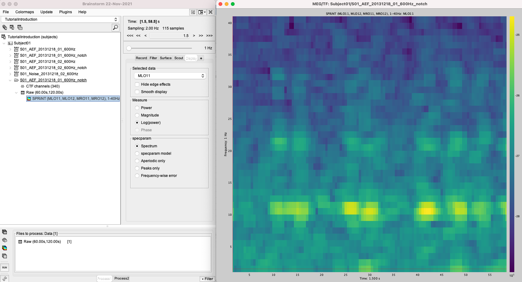
- Try all the display options:
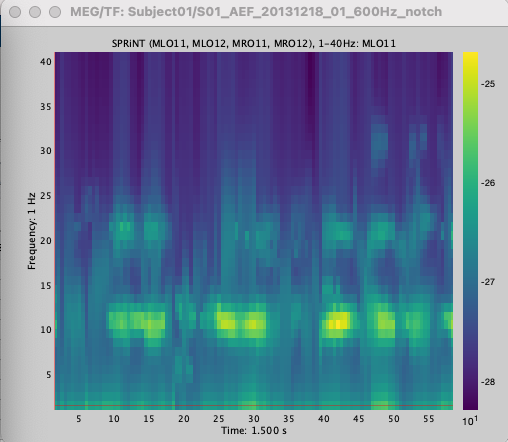
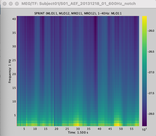
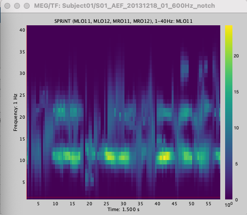
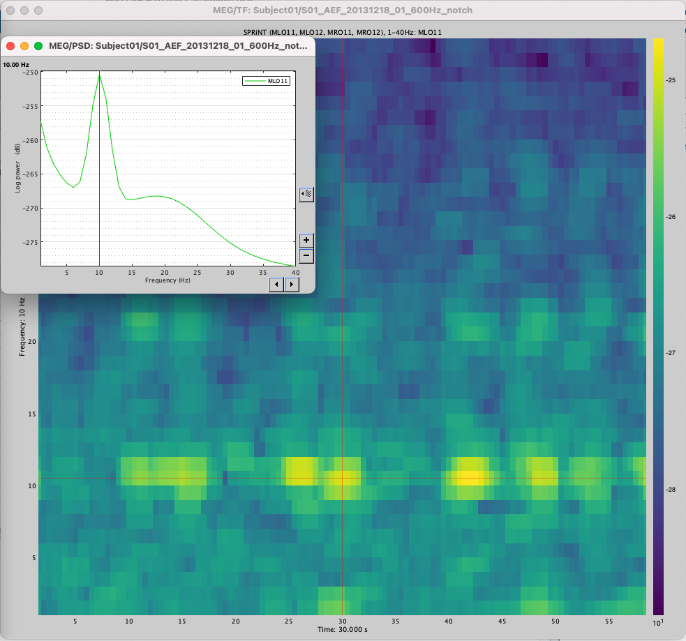
This is an ideal environment to view SPRiNT models to ensure that they are fitting the STFT map correctly. Here, you can also right-click a point in time-frequency space and select Power Spectrum to plot the spectral density at that time point. You can also separately swap the contents of this window between unmodelled spectrum (shown automatically) and SPRiNT models/components.
Accessing SPRiNT model parameters
While viewing SPRiNT maps within Brainstorm is helpful for qualitative interpretations, some may wish to extract the parameter values directly from the model for statistical tests.
Right-click on the SPRiNT file we've just created and select "File > Export to Matlab". Name the variable anything you would like (e.g., "SPRiNT_file").
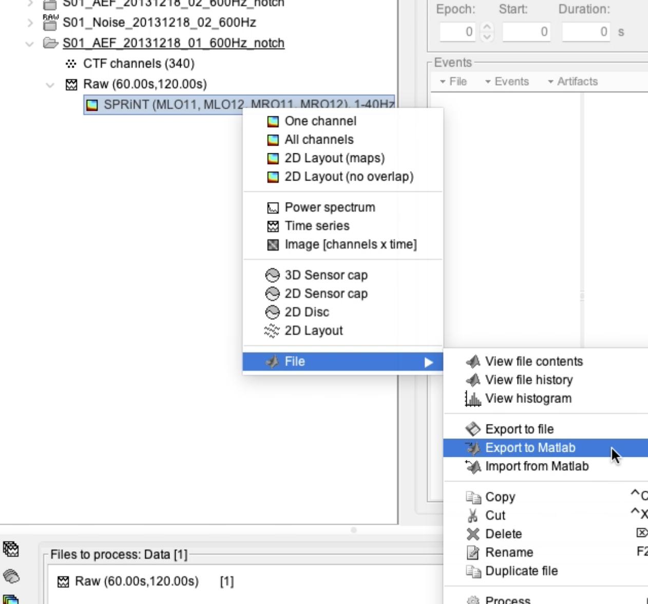
In MATLAB, you can explore the contents of the file using the tab "Workspace" (navigate to "SPRiNT_file > Options > SPRiNT") or the command line (SPRiNT_file.Options.SPRiNT).

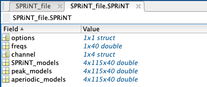
- The SPRiNT structure contains six additional elements:
options: all of the settings for the algorithm.
freqs: all of the specific frequencies used in the model.
channel: channel-specific SPRiNT data, in the same order as present in Brainstorm. Includes separate structures for all aspects of the data (data), as well as each aspect organized separately (peaks, aperiodics, stats). Data within each of these fields is organized in time. Finally, there is a field containing rough groupings of peaks for each channel across time (clustered peaks).

SPRiNT_models: a three-dimensional matrix containing power measures for each channel at each time and frequency representing full SPRiNT maps (mostly for Brainstorm visualization).
peak_models: a three-dimensional matrix containing power measures for each channel at each time and frequency representing peak components (mostly for Brainstorm visualization).
aperiodic_models: a three-dimensional matrix containing power measures for each channel at each time and frequency representing aperiodic components (mostly for Brainstorm visualization).
Acknowledgements
Please cite the SPRiNT algorithm using its associated article:
Wilson, L.E., da Silva Castanheira, J., and Baillet, S. (2022). Time-resolved parameterization of aperiodic and periodic brain activity. eLife, 11:e77348 https://doi.org/10.7554/eLife.77348
All credit for the specparam algorithm is due to Thomas Donoghue, Matar Haller, Erik Peterson, Paroma Varma, Priyadarshini Sebastian, Richard Gao, Torben Noto, Antonio H. Lara, Joni D. Wallis, Robert T. Knight, Avgusta Shestyuk, and Bradley Voytek. The appropriate citation for specparam is as follows:
Donoghue, T., Haller, M., Peterson, E.J. et al. Parameterizing neural power spectra into periodic and aperiodic components. Nat Neurosci 23, 1655–1665 (2020). https://doi.org/10.1038/s41593-020-00744-x
