|
Size: 25663
Comment:
|
Size: 26206
Comment:
|
| Deletions are marked like this. | Additions are marked like this. |
| Line 42: | Line 42: |
| Grow the scout A1L to '''40 vertices''', not in constrained mode. You can read the number of vertices and the estimated cortical area just below the [<<] and [>>] buttons.<<BR>>Then click on the second button in the ''Scout ''panel toolbar '''[Display scouts time series]'''. It displays the activation signal associated with this region for the entire time window (-100ms to 500ms). . {{attachment:scout_display.gif}} == Display options == |
Grow the scout A1L to '''40 vertices''', not in constrained mode. You can read the number of vertices and the estimated cortical area just below the [<<] and [>>] buttons. . {{attachment:scout_grow.gif||height="159",width="529"}} ==== Display time series ==== Select the souct in the list, click on the second button in the toolbar '''[Display scouts time series]'''. It displays the signal associated with this region for the entire time window (-100ms to 500ms). <<BR>>We can now observe the early response at 50ms (P50) that was not very obvious before. . {{attachment:scout_display.gif||height="153",width="420"}} == 3D display options == |
| Line 53: | Line 58: |
| * If both previous buttons are unselected: no scouts are displayed in the 3D figure. It can be interesting to hide all the scouts if you are working with atlases on hi-resolution surfaces and if it takes to long to open a surface. | * '''Hide all''': Uncheck both buttons above to hide the scouts in the 3D figure. |
| Line 63: | Line 68: |
| How are the scouts time series calculated? For the scout LeftSS we have 15 signals, coming from 15 different dipoles with different orientations, that are combined into one unique signal. In the list of available scouts, you can see the indication "[mean]" next to the name of the scout. It represents the name of the function that is used for combined all the time series into one. This function can be changed individually for each scout, with the menu ''Scout > Set function'' in the Scout tab. ==== List of the functions ==== |
We have added '''40 vertices''' the scout '''A1L'''. Because we are computed a source model with unconstrained dipoles orientations, we have three sources per vertex. This region A1L corresponds to '''120 signals'''. The signals are grouped together into one unique signal that is then used to represent the activity of the region of interest. In the list of available scouts, you can see the indication '''[Mean]''' next to the name of the scout. It represents the name of the function that is used for combining all the source signals into one. This function can be changed individually for each scout, with the menu '''Scout > Set function'''. |
| Line 68: | Line 74: |
| * '''Mean''': Average all the signals | * '''Mean''': Average all the signals. |
| Line 71: | Line 77: |
| * '''Mean(norm)''': Average the absolute values of all the signals * '''Max''': For each time point, get the maximum across all the vertices [signed maximum in amplitude value: m = max(abs(signal)), scout = sign(signal(m)) * m] * '''Power''': Average the power of all the signals (signal^2) * '''All''': Do not apply any operation on the scouts signals, and display the time series of all the sources at the same time. ==== "Absolute" display option ==== As said in the previous tutorial, the minimum norm current amplitudes can positive or negative. Which means that the values of the scouts, depending on the function that is used, may be positive or negative too. Most of the time we are interested in visualizing the absolute values of the scouts time series, to compare the activation level in different conditions or subjects. For this purpose, at the bottom of the Scout tab, you can choose to display either ''Absolute ''or ''Relative ''values. The effect of this options depends if you are processing sources with constrained (1 signal per vertex) or unconstrained (3 signals per vertex) orientations: * '''Constrained''': Applies the scout function ''sfunction'' to all the N sources time series, and then apply or not an absolute value * '''Absolute''': abs(sfunction(sources)) * '''Relative''': sfunction(sources) * '''Unconstrained''': Applies the scout function ''sfunction ''to the N sources time series for each orientation (x,y,z) separately, and then returns either the norm of the 3 orientations, or each orientation separately * '''Absolute''': Returns __one__ time series: <<BR>>sqrt( sfunction(sources_x).<<HTML(^)>>2 + sfunction(sources_y).<<HTML(^)>>2 + sfunction(sources_z).<<HTML(^)>>2) * '''Relative''': Returns __three__ time series: <<BR>>sfunction(sources_x), sfunction(sources_y), sfunction(sources_z) Change the selection to ''Relative ''and display again the activation of scout LeftSS for condition Right. {{attachment:absButton.gif}} The effect of the function depends if you are processing sources with constrained (1 signal per vertex) or unconstrained (3 signals per vertex) orientations. Note that it is a display option, it is not saved in the scouts themselves. It is used ONLY when displaying the scouts time series with the "Display" button of the Scout tab. In all other cases, like the extraction of the scouts values from a script, this relative/absolute option is going to be ignored. ==== Testing the functions ==== Now, leave this ''Relative'' option selected for testing all the scouts functions one by one. {{attachment:compFunc.gif}} Select again the "''Absolute''" display again, and keep it for the rest of the tutorial. == Multiple scouts == We are going to create another scout for the other condition: the stimulation of the '''left thumb'''. 1. Close all figures (toolbar button). 1. Display the times series for ''Subject01 / '''Left '''/ ERF'' (double-click). 1. Display the associated sources (Ctrl+S). 1. Go to the main response peak (46 ms). 1. Adjust the threshold value to get only a very focal point (about 60%). 1. Create a new scout at this point. Name it ''RightSS'', for Right SomatoSensory cortex. 1. Grow it to the same number of vertices as the ''LeftSS ''scout (about 15 vertices). 1. Select both scouts (Ctrl+click) and click on ''Display scouts time series'' button (second button in toolbar).<<BR>><<BR>> {{attachment:scouts2.gif}} <<BR>><<BR>> {{attachment:scoutsTS_LR.gif}} 1. You can display the values of the two scouts on the same graph. Check the ''Overlay > Scouts'' checkbox in the Scout tab, and hit the ''Display scouts time series'' button again.<<BR>><<BR>> {{attachment:scoutsTS_LR_overlay.gif}} 1. You can observe something that we expected: the activity in the '''right somatosensory cortex''' is much higher than in the left somatosensory cortex for a stimulation of the '''left thumb'''. == Display scouts from the database explorer == You have to display the sources on the cortex to create the scouts. But once they are created, you can directly display the scouts time series from the tree. It means that you can quickly compare the values for a scout between many different conditions without having to open them all. 1. Close all the figures (button in toolbar) 1. Select the options "values: absolute" and "overlay: scouts" 1. Right-click on '''Right '''/ ERF / MN > Cortical activations > Scouts time series.<<BR>>By default it shows all the scouts that are available in the current atlas.<<BR>><<BR>> {{attachment:treeRight.gif}} <<BR>> {{attachment:treeRight_TS.gif}} 1. Note that if a surface is loaded, and at least one scout selected in the ''Scout'' tab, this popup menu would display only the selected scouts. 1. You can also display the scout values for many source files at the same time. Now keep the previous figure opened, so you have access to the scouts list in the ''Scout'' tab. Select only the ''LeftSS'' scout. In the database explorer, select at the same time the source files from condition Left and Right > right-click > Cortical activations > Scouts time series.<<BR>><<BR>> {{attachment:treeLR.gif}} <<BR>> {{attachment:treeLR_TS.gif}} 1. You can superimpose the two traces from the two experimental conditions by selecting the ''Overlay > Conditions'' checkbox in ''Scout ''panel. Select again the two files > Right click > Scouts time series. We see now the activation of the LeftSS scout for the stimulation of both thumbs.<<BR>><<BR>> {{attachment:panelOverlayCond.gif}} 1. This menu "Scouts time series" is present at all the levels in the tree. Try right-clicking on Subject01 > Scouts time series. 1. If you select a node in the database tree and click on the ''Display scouts time series'' button in the ''Scout ''tab, it would have exactly the same effect. <<BR>>Try selecting '''both scouts''' in the list, select '''Subject01 '''in the tree, overlay / conditions, and then click on this button. You will see the response for each scout in both conditions.<<BR>><<BR>> {{attachment:scoutsOverlayBoth.gif}} == Scout toolbar and menus == Let's spend a few minutes to explore all the menus in the ''Scout ''tab. Don't hesitate to click on all of them, it's the best way to remember what they do. === Menu: Atlas === . {{attachment:menuNew.gif}} * '''New atlas''': Create a new empty atlas. * '''Load atlas''': Load ROIs or a cortical parcellation coming from FreeSurfer or BrainSuite as a new atlas. * '''Rename atlas''': Change the name that appears in the atlas list to refer to the selected atlas * '''Delete atlas''': Delete the atlas and all the scouts in contains. The "User scouts" entry cannot be deleted. * '''Add scouts to atlas''': Load ROIs or a cortical parcellation and add them to the current atlas. * '''Copy atlas''': Duplicates an atlas and all the scouts * '''Copy selected scouts''': Copy the selected scouts, and paste them in a new empty atlas. * '''Subdivide atlas''': Splits all the scouts of the current atlas in smaller ROIs. Available options:<<BR>><<BR>> {{attachment:scoutSubdivide.gif}} * '''Subdivide selected scouts''': Same thing, but processes only the selected scouts. * '''Surface clustering''': Create a parcellation of the cortex surface and saves it as a new atlas. Can be useful for studying the connectivity between different regions of the brain. Only the "Random" clustering is currently available. Experimental features. === Menu: Scout === . {{attachment:menuEdit.gif}} * '''Add vertices''': The user can select some points on the cortex surface and add them to the scout.<<BR>>Equivalent: Click on ''Select point'' (first toolbar button), then select the scout in list, and select 3d points. * '''Edit in MRI''': Open an interface to edit the select scout as a 3D ROI, slice by slice. * Define the 3D mask using the drawing tools (read the tooltips of the buttons for help). * Adjust the MRI contrast with right-click+move on the MRI image. * Move through the slices with the mouse wheel, the small image on the left, or the slider. * __Warning__: Only the vertices contained in the 3D mask are kept, all the volume information is lost. It means that the mask you intendend to draw might be very different from what you get as a scout at the end...<<BR>><<BR>> {{attachment:menuEditMriMask.gif}} * '''Set function''': Set the scout function for the selected scouts. * '''Set region''': Set the cortical region for the selected scouts. This information is useful when representing functional connectivity graphs. * '''Rename''': Rename the selected scout. Shortcut: ''double-click''. * '''Set color''': Change the display color of scout patch in 3D figures. * '''Delete''': Delete selected scouts. Shortcut: ''Delete'' key * '''Merge''': Join two or more selected scouts. * '''Export to Matlab''': Export the structures of the selected scouts to the Matlab environment, and makes them accessible from the command window. This menu can be useful to get quickly the list of vertices in the scout. * '''Import from Matlab''': Import scouts structures that you modified manually from your Matlab command window directly as new scouts. * '''Edit surface''': Create a new surface containing only the desired parts (remove or keep only the selected scouts). This is useful for instance for selecting one sub-cortical region from the Aseg FreeSurfer atlas (see the [[Tutorials/LabelFreeSurfer|FreeSurfer tutorial]]). === Menu: Sources === . {{attachment:menuView.gif}} * '''Simulate recordings''': Multiply the selected scouts with the forward model. Simulate the scalp data that would be recorded if only the selected cortex region was activated; all the other sources are set to zero. Create a new data file in the database.<<BR>>If no scout selected: simulate recordings produced by the activity of the entire cortex. * '''Correlation with sensor''': Create a new scout with all the sources that are strongly correlated with a given sensor. * '''Expand with correlation''': Computes the correlation between the values for the scout's seed (first point) and all the other sources. The sources that have correlation coefficient superior to a given threshold are added to the scout. Correlation is computed with the Matlab ''corrcoef ''function. * '''Maximal value (new scout)''': Find the vertex with the maximal intensity at the current time, and create a scout centered on it. * '''Maximal value (selected scout)''': Move the scout's seed to the source that has the maximum amplitude in the scout, at the current time. == Scout region == A scout is defined by its name, and it has several properties: a list of vertices and an aggregating function. These are usually enough to explore the activity at the cortex level the way we did it in these tutorials. An extra property can be defined on the scout: the explicit classification in a brain region. This property is used only in more advanced functional connectivity analysis, for the representation of the NxN connection graphs. It is introduced here for reference purpose. A brain region in Brainstorm is following a hierarchy with three levels: hemisphere / lobe / sub-region. The definition at each level is optional: a region can be classified only at the hemisphere level, or at the hemisphere+lobe level, or none of them. It depends on level or hierarchy you are interested in to explore the connectivity graphs. The region for a scout can be set with the ''Scout > Set region'' menus, and is encoded in a string that contains at least 2 characters: "'''HLxxx'''". H represents the hemisphere (L,R,U), L stands for the lobe (F,PF,C,P,T,O,L,U), and xxx for the sub-region name (optional). For both the hemisphere and the lobe, the value "U" stands for "Undefined", meaning that the classification is simply not set. The menu ''Set region>Custom region...'' lets you edit this string directly. The menu ''Set region>Undefined ''sets the region string to "UU" (undefined hemisphere, undefined lobe). When set, the region string is shown before the scout name in the list, representing only the defined levels. It doesn't show the letters U for "undefined", therefore the scouts you create manually, that are by default set to "UU", do not show any extra string. . {{attachment:menuRegions.gif}} = From auditory = == Regions of interest == === Manual tracing === |
* '''Mean(norm)''': Average the absolute values of all the signals: mean(abs(signal)) * '''Max''': For each time point, get the maximum across all the vertices.<<BR>>Signed maximum: m = max(abs(signal)), scout = sign(signal(m)) * m * '''Power''': Average the square of all the signals: mean(signal^2) * '''All''': Do not apply any operation on the scouts signals, returns all the signals. <<BR>><<BR>> {{attachment:scout_all.gif||height="146",width="447"}} == Option: Absolute / relative == As said in the previous tutorial, the minimum norm current amplitudes can positive or negative depending on the dipole orientation. This means that the values of the scouts, depending on the function that is used, may be positive or negative too. Most of the time we are interested in visualizing the absolute values of the scouts time series, to compare the activation level in different conditions or subjects. For this purpose, at the bottom of the Scout tab, you can choose to display either ''Absolute ''or ''Relative ''values. The effect of this options depends if you are processing sources files with constrained (1 signal per vertex) or unconstrained (3 signals per vertex) dipoles orientations: * '''Constrained''': Apply the scout function to all source signals, then: * '''Absolute''': abs(ScoutFunc(sources)) * '''Relative''': ScoutFunc(sources) * '''Unconstrained''': Apply the scout function to the source signals for each orientation (x,y,z) separately, and then returns either the norm of the 3 orientations, or each orientation separately: * '''Absolute''': Returns __one__ time series: <<BR>>sqrt( ScoutFunc(sources_x).<<HTML(^)>>2 + ScoutFunc(sources_y).<<HTML(^)>>2 + ScoutFunc(sources_z).<<HTML(^)>>2) * '''Relative''': Returns __three__ time series: <<BR>>ScoutFunc(sources_x), ScoutFunc(sources_y), ScoutFunc(sources_z) '''Display only''': Note that it is a display option, it is not saved in the scouts themselves. It is used only when displaying the scouts time series with the [Display scouts time series] button of the Scout tab. In all other cases, like the extraction of the scouts values from a script, this relative/absolute option is ignored. == Relative Z-score values == Change the selection to '''Relative '''and display again the activation of scout A1L for the deviant condition. It shows only one signal because the three orientations were already grouped in the one value during the '''Z-score normalization'''. The sign of the Z-score is important to look at, because it indicates if the values are higher or lower than the baseline. With this representation, we can confirm that we only observe higher activity values than during the baseline. . {{attachment:scout_relative.gif||height="155",width="504"}} Select again the '''Absolute''' display again, and keep it for the rest of the tutorial. == Multiple conditions == We can easily compare the activity between multiple conditions and multiple regions of interest. * In ''Intra-subject'', open at the same time the normalized sources for '''deviant '''and '''standard '''condition. * Select the scout '''A1L '''and click on ['''Display soutces time series''']. <<BR>>This computes the scouts time series for all the files that are currently open.<<BR>><<BR>> {{attachment:scout_nooverlay.gif||height="126",width="451"}} * In the Record tab, you can use the button '''[=]''' to configure the amplitude of multiple axes. <<BR>>Select it to force multiple graphs to use the same scale, unselect it to scale each graph separately. <<BR>> You can find the same option in the figure popup menu: '''Figure > Uniform figure scale'''. <<BR>><<BR>> {{attachment:scout_equalamp.gif||height="126",width="450"}} * At the bottom of the Scout tab, select the option "'''Overlay: Conditions'''", then click [Display] again.<<BR>><<BR>> {{attachment:scout_overlay_cond.gif||height="143",width="607"}} * The '''Z-score value''' for the '''standard condition is a lot higher''' than the deviant condition because of the number of trials we used for computing the two averages. The SNR is higher with more trials, the baseline has less variance so the Z-score is higher. * To overlay the results of two conditions averaged with very different numbers of trials, it makes more sense to display the scout time series for non-normalized maps (averaged current density). == Other regions of interest == |
| Line 202: | Line 115: |
| * Open the average source files (standard and deviant), together with the average recordings for the standard condition for an easier time navigation. * In the Surface tab, smooth the cortical surface at '''70%'''. * For each region: go to the indicated time point, adjust the amplitude threshold in the Surface tab, identify the area of interest, click on its center, grow the scout, rename it. * Grow all the regions to the same size: '''20 vertices'''. * Note that all the following screen captures are produced with a online low-pass filter at 100Hz. * '''A1L''': Left primary auditory cortex (Heschl gyrus) * The most visible region in both conditions. Active during all the main steps of the auditory processing: P50, N100, MMN, P200, P300. * '''Standard '''condition, t='''90ms''', amplitude threshold='''70%''' {{http://neuroimage.usc.edu/brainstorm/Tutorials/Auditory?action=AttachFile&do=get&target=scout_a1l.gif|scout_a1l.gif|height="162",width="650",class="attachment"}} |
* Open the '''normalized average '''source files (standard and deviant), together with the average recordings for the deviant and standard condition for Run#01 for an easier time navigation. * In the Surface tab, smooth the cortical surface at '''60%'''. * For each region: go to the indicated time point, adjust the amplitude threshold in the Surface tab, identify the area of interest, click on its center, grow the scout, rename it. * Grow all the regions to the same size: '''40 vertices'''. * In the screen captures below, the scout times series have been computed using the '''non-normalized''' files, in order to plot the standard and deviant averages in the same graph. * '''A1L''': Left primary auditory cortex (Heschl gyrus) - Already marked. * The most visible region in both conditions. Active during all the main steps of the auditory processing: P50, N100, MMN, P200, P300. * '''Deviant '''condition, t='''90ms''', amplitude threshold='''60%''' <<BR>><<BR>> {{attachment:scout_a1l.gif||height="156",width="622"}} |
| Line 211: | Line 124: |
| * The position of this region is a lot less obvious than A1L, we don't see one focal region with a sustained activity. These binaural auditory stimulations should be generating similar bilateral responses in both left and right auditory cortices at early latencies. Possible explanations for this observation: | * The response in this region is a lot less obvious than A1L. These binaural auditory stimulations should be generating similar responses in both left and right auditory cortices at early latencies. Possible explanations for this observation: |
| Line 215: | Line 128: |
| * The orientation of the source makes it difficult to capture for the MEG sensors. * We are trying to find a region that peaks at the same time as A1L (95ms and 200ms in the standard condition). It is very difficult to find anything that behaves this way in both the deviant and the standard condition, so we will pick something very approximate, knowing that we cannot really rely on this region. The auditory system is very dynamic, in squared centimeters of cortex we can observe many functionally independent regions activated at different moments. * '''Deviant '''condition, t='''34ms''', amplitude threshold='''20%''' * Results are ok for the deviant condition but not so good for the standard condition. {{http://neuroimage.usc.edu/brainstorm/Tutorials/Auditory?action=AttachFile&do=get&target=scout_a1r.gif|scout_a1r.gif|height="162",width="648",class="attachment"}} |
* The orientation of the source makes it difficult for the MEG sensors to capture. * '''Deviant '''condition, t='''90ms''', amplitude threshold='''40% '''<<BR>><<BR>> {{attachment:scout_a1r.gif||height="156",width="622"}} |
| Line 223: | Line 133: |
| * '''Deviant '''condition, t='''140ms''', amplitude threshold='''40% ''' {{http://neuroimage.usc.edu/brainstorm/Tutorials/Auditory?action=AttachFile&do=get&target=scout_ifgl.gif|scout_ifgl.gif|height="162",width="648",class="attachment"}} * '''IFGR''': Right inferior frontal gyrus (Brodmann area 44''')''' * Expected to have an activity similar to the left IFG. * '''Deviant '''condition, t='''110ms''', amplitude threshold='''40% ''' {{http://neuroimage.usc.edu/brainstorm/Tutorials/Auditory?action=AttachFile&do=get&target=scout_ifgr.gif|scout_ifgr.gif|height="162",width="648",class="attachment"}} |
* '''Deviant '''condition, t='''130ms''', amplitude threshold='''30% '''<<BR>><<BR>> {{attachment:scout_ifgl.gif||height="156",width="622"}} |
| Line 229: | Line 136: |
| * The motor cortex responds at very early latencies together with the auditory cortex, in both conditions (50ms and 100ms). The subject is ready for a fast response to the task. * At 175ms, the peak in the deviant condition probably corresponds to an inhibition: the sound heard is not a deviant, there is no further motor processing required. * At 225ms, the peak in the standard condition is probably a motor preparation. At 350ms, the motor task begins, the subject moves the right hand (recorded reaction times 500ms +/- 108ms). * '''Deviant '''condition, t='''240ms''', amplitude threshold='''50% ''' {{http://neuroimage.usc.edu/brainstorm/Tutorials/Auditory?action=AttachFile&do=get&target=scout_m1l.gif|scout_m1l.gif|height="162",width="648",class="attachment"}} * '''M1R''': Right motor cortex * Probably involved in the preparation of the motor response as well. Less recruited during the actual motor command. * '''Deviant '''condition, t='''35ms''', amplitude threshold='''25%'''''' ''' {{http://neuroimage.usc.edu/brainstorm/Tutorials/Auditory?action=AttachFile&do=get&target=scout_m1r.gif|scout_m1r.gif|height="162",width="648",class="attachment"}} |
* The motor cortex responds at very early latencies together with the auditory cortex, in both conditions (50ms and 100ms). The subject is ready for a fast response to the task. * At 170ms, the peak in the standard condition probably corresponds to an inhibition: the sound heard is not a deviant, there is no further motor processing required. * At 240ms, the peak in the standard condition is probably a motor preparation. At 350ms, the motor task begins, the subject moves the right hand (recorded reaction times 500ms +/- 108ms). * We cannot expect to have clear responses during the motor response because of the averaging. The response times are variable, so in order to get a better representation of the regions involved we should import and average the trials based on the response triggers. * '''Standard '''condition, t='''170ms''', amplitude threshold='''60%''' <<BR>><<BR>> {{attachment:scout_m1l.gif||height="156",width="622"}} * '''SMAL''': Left supplementary motor area * Probably involved in the preparation and control of the motor response as well. * '''Deviant '''condition, t='''440ms''', amplitude threshold='''35%'''''' '''<<BR>><<BR>> {{attachment:scout_smal.gif||height="156",width="622"}} |
| Line 238: | Line 146: |
| * '''Deviant '''condition, t='''225ms''', amplitude threshold='''60%'''''' ''' {{http://neuroimage.usc.edu/brainstorm/Tutorials/Auditory?action=AttachFile&do=get&target=scout_ppcr.gif|scout_ppcr.gif|height="163",width="652",class="attachment"}} | * '''Standard '''condition, t='''250ms''', amplitude threshold='''25%'''''' '''<<BR>><<BR>> {{attachment:scout_ppcr.gif||height="156",width="622"}} <<TAG(Advanced)>> == Multiple scouts == We can display the activity of multiple regions simulatenously. * Close everything (toolbar button [X]). * Open the two '''non-normalized average '''source files (standard and deviant). * In the Scout tab, select the '''A1L '''and '''IFGL '''scouts simultaneously. * Select the option "'''Overlay:Scouts'''", do not select "Overlay:Conditions" * Click on ['''Display scouts time series'''].<<BR>><<BR>> {{attachment:overlay_scouts.gif||height="142",width="490"}} * Now select the option "'''Overlay:Conditions'''", do not select "Overlay:Scouts", click on ['''Display''']. <<BR>><<BR>> {{attachment:overlay_conditions.gif||height="143",width="491"}} * In both conditions, we observe similar early responses (P50 and N100), then it diverges.<<BR>><<BR>>In the deviant condition, we observe a pattern A1-IFG-A1 that is absent in the standard conditions. * More scouts, deviant condition, '''current density''': <<BR>><<BR>> {{attachment:scout_all_mne.gif||height="142",width="490"}} * Same scouts, deviant condition, '''Z-score'''. The signals are the same but scaled differently.<<BR>><<BR>> {{attachment:scout_all_zscore.gif||height="143",width="490"}} <<TAG(Advanced)>> == From the database explorer == You have to display the sources on the cortex to create the scouts. But once they are created, you can directly display the scouts time series from the tree. It means that you can quickly compare the values for a scout between many different conditions without having to open them all. * Close everything (toolbar button [X]). * Select the option "'''Overlay:Conditions'''", do not select "Overlay:Scouts". * Select the two average recordings in Run#01 folder > right-click > '''Scouts time series'''. <<BR>>Note that this menu is present at all the levels in the database explorer.<<BR>><<BR>> {{attachment:scout_tree_popup.gif||height="277",width="456"}} * If no scout is currently loaded in the Scout tab, it shows all the scouts available in the surface. <<BR>>If a surface is loaded, and at least one scout selected in the Scout tab, this popup menu would display only the selected scouts. <<BR>><<BR>> {{attachment:scout_tree.gif||height="223",width="452"}} <<TAG(Advanced)>> == Unconstrained sources == * Open any of the '''non-normalized''' source files in your database (average current density). * Select the option "'''Values: Relative'''", display the first scout in the list (A1L): <<BR>><<BR>> {{attachment:scout_unconstr.gif||height="157",width="606"}} * It shows three graphs, corresponding to the three dipole orientations: A1L1='''X''', A1L2='''Y''', A1L3='''Z''' <<TAG(Advanced)>> == Scout toolbar and menus == === Menu: Atlas === . {{attachment:menu_atlas.gif}} * '''New atlas''': * '''Empty atlas''': Create a new empty atlas. * '''Copy atlas''': Duplicates an atlas and all the scouts it contains. * '''Copy selected scouts''': Create a new atlas and copy only the selected scouts to it. * '''Source model options''': Create a special atlas "Source model", with which you can attribute different modeling constraints to each region. Create after merging the cortex with some subcortical regions. This is required to use the option "'''Custom head model'''" (mixed models). * '''Volume scouts''': Create a volume atlas in order to store 3D scouts (volume head models). * '''Load atlas''': Load ROIs or a cortical parcellation coming from FreeSurfer or BrainSuite as a new atlas. * '''Rename atlas''': Change the name that appears in the atlas list to refer to the selected atlas. * '''Delete atlas''': Delete the current atlas and all the scouts in contains. * '''Add scouts to atlas''': Load ROIs or a cortical parcellation and add them to the current atlas. * '''Subdivide atlas''': Splits all the scouts of the current atlas in smaller ROIs. Available options:<<BR>><<BR>> {{attachment:scoutSubdivide.gif||height="146",width="298"}} * '''Subdivide selected scouts''': Same thing, but processes only the selected scouts. * '''Surface clustering''': Create a parcellation of the cortex surface and saves it as a new atlas. <<BR>>Only the "Homogeneous parcellation" clustering is currently available. * '''Save modifications''': Force the current modifications to be saved to the cortex surface. * '''Undo all modifications''': Restore the atlas the way it was the last time the surface was loaded. === Menu: Scout === . {{attachment:menu_scout.gif}} * '''New: coordinates''': Create a new scout starting from the vertex that is the closest to the specified coordinates. You can enter coordinates in MRI, SCS or MNI coordinates. * '''Add vertices''': The user can select some points on the cortex surface and add them to the scout.<<BR>>Equivalent: Click on ''Select point'' (first toolbar button) then select the scout in list. * '''Edit in MRI''': Open an interface to edit the select scout as a 3D ROI, slice by slice. Only the vertices contained in the 3D mask are kept, all the volume information is lost. It means that the mask you intendend to draw might be very different from what you get as a scout at the end. This is not a very reliable tool, as there is no direct correspondence between the volume and the surface. * '''Set function''': Set the scout function for the selected scouts. * '''Set region''': Set the cortical region for the selected scouts. * '''Rename''': Rename the selected scout. Shortcut: '''double-click'''. * '''Set color''': Change the display color of scout patch in 3D figures. * '''Delete''': Delete selected scouts. Shortcut: '''Delete '''key * '''Merge''': Join two or more selected scouts. * '''Export to Matlab''': Export the structures of the selected scouts to the Matlab environment and makes them accessible from the command window. This menu can be useful to get quickly the list of vertex indices or modify a scout manually. * '''Import from Matlab''': Import scouts structures that you modified manually from your Matlab command window directly as new scouts. * '''Project to''': Project the selected scout on another surface available in the database. * '''Edit surface''': Create a new surface containing only the desired parts (remove or keep only the selected scouts). This is useful for instance for selecting one sub-cortical region from the Aseg FreeSurfer atlas (see the [[Tutorials/LabelFreeSurfer|FreeSurfer tutorial]]). === Menu: Sources === . {{attachment:menu_sources.gif}} * '''Correlation with sensor''': Create a new scout with all the sources that are strongly correlated with a given sensor. * '''Expand with correlation''': Computes the correlation between the values for the scout's seed (first point) and all the other sources. The sources that have correlation coefficient superior to a given threshold are added to the scout. * '''Maximal value (new scout)''': Find the vertex with the maximal intensity at the current time, and create a scout centered on it. * '''Maximal value (selected scout)''': Move the scout's seed to the source that has the maximum amplitude in the scout, at the current time. * '''Simulate recordings''': Multiply the selected scouts with the forward model. Simulate the scalp data that would be recorded if only the selected cortex region was activated; all the other sources are set to zero. Create a new data file in the database.<<BR>>If no scout selected: simulate recordings produced by the activity of the entire cortex. <<TAG(Advanced)>> == Scout region == A scout is defined by its name, and it has several properties: a list of vertices and an aggregating function. These are usually enough to explore the activity at the cortex level the way we did it in these tutorials. An extra property can be defined on the scout: the explicit classification in a brain region. This property is used only in more advanced functional connectivity analysis, for the representation of the NxN connection graphs. It is introduced here for reference purpose. A brain region in Brainstorm is following a hierarchy with three levels: hemisphere / lobe / sub-region. The definition at each level is optional: a region can be classified only at the hemisphere level, or at the hemisphere+lobe level, or none of them. It depends on level or hierarchy you are interested in to explore the connectivity graphs. The region for a scout can be set with the ''Scout > Set region'' menus, and is encoded in a string that contains at least 2 characters: "'''HLxxx'''". H represents the hemisphere (L,R,U), L stands for the lobe (F,PF,C,P,T,O,L,U), and xxx for the sub-region name (optional). For both the hemisphere and the lobe, the value "U" stands for "Undefined", meaning that the classification is simply not set. The menu ''Set region>Custom region...'' lets you edit this string directly. The menu ''Set region>Undefined ''sets the region string to "UU" (undefined hemisphere, undefined lobe). When set, the region string is shown before the scout name in the list, representing only the defined levels. It doesn't show the letters U for "undefined", therefore the scouts you create manually, that are by default set to "UU", do not show any extra string. . {{attachment:scout_region.gif}} <<TAG(Advanced)>> |
| Line 241: | Line 262: |
| The scouts are saved in the surface file on which they have been defined.<<BR>> In the anatomy view, right-click on the selected cortex surface (cortex_15002V) > View file contents. {{attachment:scout_harddrive.gif}} Fields in the surface files: * |
Tutorial 23: Scouts
Authors: Francois Tadel, Elizabeth Bock, John C Mosher, Richard Leahy, Sylvain Baillet
In Brainstorm jargon, a scout represents a region of interest (ROI) in the available source space. It is a subset of dipoles defined on the cortex surface or the head volume. This tutorial explains how to create one or several scouts, use them to represent the activity in specific brain regions and compare the responses between different experimental conditions.
Contents
Hypothesis
For all the brain imaging experiments, it is highly recommended to have a clear hypothesis to test before starting the analysis of the recordings. With this auditory oddball experiment, we would like to explore the temporal dynamics of the auditory network, the deviant detection and the motor response. According to the literature, we expect to observe at least the following effects:
Bilateral response in the primary auditory cortex (P50, N100), in both experimental conditions (standard and deviant beeps).
Bilateral activity in the inferior frontal gyrus and the auditory cortex corresponding to the detection of an abnormality (latency: 150-250ms) for the deviant beeps only.
Decision making and motor preparation, for the deviant beeps only (after 300ms).
We will start by creating regions of interest corresponding to the auditory cortices to illustrate the tools, then define other regions to explore better the dynamics of the brain response.
Creating a scout
Almost all the features related to the scouts manipulation are accessible in the Scout tab in the main Brainstorm window. The scouts are automatically saved in the surface file from which they are created, and they are loaded and automatically displayed each time the surface is loaded.
An atlas designates in this context a list of scouts. For one cortex surface, we can have as many atlases as needed. An atlas can be an anatomical parcellation (like the ones loaded when using FreeSurfer), a random parcellation generated by Brainstorm, or a user-defined list of ROIs. All the surfaces contain by default an empty atlas called "User scouts", for the user to create new regions of interest.
First vertex (seed)
In Intra-subject, double-click on the standardized deviant average.
In Run#01, open the average recordings for the deviant condition, to have a time reference.
Go to the first peak in the deviant response, around 90ms.
In the Surface tab, increase the amplitude threshold to see something relatively focal. The response is larger in the left hemisphere, so let's start with the left.

Switch to the Scout tab, click on the first button in the toolbar (the big cross).
In the 3D figure, click where we expect to find the primary auditory cortex (rotate and zoom before if necessary). A small green dot with the label "1" appears where you clicked. Your first scout is created in the User scouts atlas, and contains only one vertex for the moment.
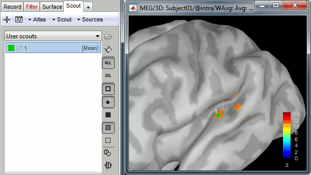
If you are not satisfied with the position of the vertex you selected, delete the new scout (select it in the list and press the Delete key, or menu Scout > Delete) and try again.
Rename it "A1L", for primary auditory left: double-click on it in the list, or menu Scout > Rename.
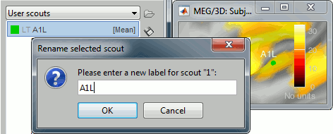
In light grey, you can see in the list the letters "LT", this means that based on the anatomical atlases imported from FreeSurfer, the point you clicked is in the left temporal lobe.
Growing a scout
For now, our scout contains only one vertex of the cortex surface. Most of the time, the aim of a scout is to extract the average activity over a larger region. The buttons in the Scout size section offer basic operations to define the scout extension.
[>]: Add the closest vertex (with respect to the seed) to the current scout.
[<]: Remove the furthest vertex (with respect to the seed) from the current scout.
[>>]: Grow scout in all directions.
[<<]: Shrink scout in all directions.
'Constrained': If this button is pressed, only the vertices that have a source value above the threshold will be added to the scout (its growth will be limited to the colored patch on the surface).
Add vertex manually: Select the Select point button, then select again the "A1L" scout. When you click on a vertex on the surface, it is added to the selected scout.
Remove vertex manually: Same as previously, but holding the SHIFT key at the same time.
Grow the scout A1L to 40 vertices, not in constrained mode. You can read the number of vertices and the estimated cortical area just below the [<<] and [>>] buttons.
Display time series
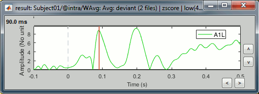
Select the souct in the list, click on the second button in the toolbar [Display scouts time series]. It displays the signal associated with this region for the entire time window (-100ms to 500ms).
We can now observe the early response at 50ms (P50) that was not very obvious before.
3D display options
In the toolbar on the right side of scouts tab, you can find a list display options. Leave your mouse over it for a few seconds to get a description of each of them.
 Load Atlas
  Save selected scouts
  Show all the scouts
  Show only the selected scouts
 Hide all: Uncheck both buttons above to hide the scouts in the 3D figure.
 Show / hide the contour line
  Show / hide the scouts labels
  Scout patch: Opaque
  Scout patch: Transparent
  Scout patch: None
  Display the color of the region instead of the scout color (only for anatomical atlases)
  Center MRI on scout (opens the MRI viewer and set the position to the current scout)
Scout function
We have added 40 vertices the scout A1L. Because we are computed a source model with unconstrained dipoles orientations, we have three sources per vertex. This region A1L corresponds to 120 signals.
The signals are grouped together into one unique signal that is then used to represent the activity of the region of interest. In the list of available scouts, you can see the indication [Mean] next to the name of the scout. It represents the name of the function that is used for combining all the source signals into one. This function can be changed individually for each scout, with the menu Scout > Set function.
Here is a description of the different options. In the case of unconstrained sources (3 signals for each vertex, one for each orientation), the function is applied separately for each orientation and produces 3 time series instead of one. For more details, see the code of bst_scout_value.m.
Mean: Average all the signals.
PCA: Take the first mode of the PCA decomposition of all the signals.
Fast PCA: Same as PCA function, but computes the first PCA decomposition based only on a subset of the most powerful signals. It gives very similar results, but its computation is much faster for scouts that group a large number of dipoles (>50).
Mean(norm): Average the absolute values of all the signals: mean(abs(signal))
Max: For each time point, get the maximum across all the vertices.
Signed maximum: m = max(abs(signal)), scout = sign(signal(m)) * mPower: Average the square of all the signals: mean(signal^2)
All: Do not apply any operation on the scouts signals, returns all the signals.

Option: Absolute / relative
As said in the previous tutorial, the minimum norm current amplitudes can positive or negative depending on the dipole orientation. This means that the values of the scouts, depending on the function that is used, may be positive or negative too. Most of the time we are interested in visualizing the absolute values of the scouts time series, to compare the activation level in different conditions or subjects.
For this purpose, at the bottom of the Scout tab, you can choose to display either Absolute or Relative values. The effect of this options depends if you are processing sources files with constrained (1 signal per vertex) or unconstrained (3 signals per vertex) dipoles orientations:
Constrained: Apply the scout function to all source signals, then:
Absolute: abs(ScoutFunc(sources))
Relative: ScoutFunc(sources)
Unconstrained: Apply the scout function to the source signals for each orientation (x,y,z) separately, and then returns either the norm of the 3 orientations, or each orientation separately:
Absolute: Returns one time series:
sqrt( ScoutFunc(sources_x).^2 + ScoutFunc(sources_y).^2 + ScoutFunc(sources_z).^2)Relative: Returns three time series:
ScoutFunc(sources_x), ScoutFunc(sources_y), ScoutFunc(sources_z)
Display only: Note that it is a display option, it is not saved in the scouts themselves. It is used only when displaying the scouts time series with the [Display scouts time series] button of the Scout tab. In all other cases, like the extraction of the scouts values from a script, this relative/absolute option is ignored.
Relative Z-score values
Change the selection to Relative and display again the activation of scout A1L for the deviant condition. It shows only one signal because the three orientations were already grouped in the one value during the Z-score normalization. The sign of the Z-score is important to look at, because it indicates if the values are higher or lower than the baseline. With this representation, we can confirm that we only observe higher activity values than during the baseline.
Select again the Absolute display again, and keep it for the rest of the tutorial.
Multiple conditions
We can easily compare the activity between multiple conditions and multiple regions of interest.
In Intra-subject, open at the same time the normalized sources for deviant and standard condition.
Select the scout A1L and click on [Display soutces time series].
This computes the scouts time series for all the files that are currently open.

In the Record tab, you can use the button [=] to configure the amplitude of multiple axes.
Select it to force multiple graphs to use the same scale, unselect it to scale each graph separately.
You can find the same option in the figure popup menu: Figure > Uniform figure scale.
![[ATTACH] [ATTACH]](/moin_static1911/brainstorm1/img/attach.png)
At the bottom of the Scout tab, select the option "Overlay: Conditions", then click [Display] again.

The Z-score value for the standard condition is a lot higher than the deviant condition because of the number of trials we used for computing the two averages. The SNR is higher with more trials, the baseline has less variance so the Z-score is higher.
- To overlay the results of two conditions averaged with very different numbers of trials, it makes more sense to display the scout time series for non-normalized maps (averaged current density).
Other regions of interest
- Let's place all the regions of interest starting from the easiest to identify.
Open the normalized average source files (standard and deviant), together with the average recordings for the deviant and standard condition for Run#01 for an easier time navigation.
In the Surface tab, smooth the cortical surface at 60%.
- For each region: go to the indicated time point, adjust the amplitude threshold in the Surface tab, identify the area of interest, click on its center, grow the scout, rename it.
Grow all the regions to the same size: 40 vertices.
In the screen captures below, the scout times series have been computed using the non-normalized files, in order to plot the standard and deviant averages in the same graph.
A1L: Left primary auditory cortex (Heschl gyrus) - Already marked.
A1R: Right primary auditory cortex (Heschl gyrus)
- The response in this region is a lot less obvious than A1L. These binaural auditory stimulations should be generating similar responses in both left and right auditory cortices at early latencies. Possible explanations for this observation:
- The earplug was not adjusted on the right side and the sound was not well delivered.
- The subject's hearing from the right ear is impaired.
- The response is actually stronger in the left auditory cortex for this subject.
- The orientation of the source makes it difficult for the MEG sensors to capture.
- The response in this region is a lot less obvious than A1L. These binaural auditory stimulations should be generating similar responses in both left and right auditory cortices at early latencies. Possible explanations for this observation:
IFGL: Left inferior frontal gyrus (Brodmann area 44)
M1L: Left motor cortex
- The subject taps with the right index when a deviant is presented.
- The motor cortex responds at very early latencies together with the auditory cortex, in both conditions (50ms and 100ms). The subject is ready for a fast response to the task.
- At 170ms, the peak in the standard condition probably corresponds to an inhibition: the sound heard is not a deviant, there is no further motor processing required.
- At 240ms, the peak in the standard condition is probably a motor preparation. At 350ms, the motor task begins, the subject moves the right hand (recorded reaction times 500ms +/- 108ms).
- We cannot expect to have clear responses during the motor response because of the averaging. The response times are variable, so in order to get a better representation of the regions involved we should import and average the trials based on the response triggers.
SMAL: Left supplementary motor area
PPCR: Right posterior parietal cortex
Multiple scouts
We can display the activity of multiple regions simulatenously.
- Close everything (toolbar button [X]).
Open the two non-normalized average source files (standard and deviant).
In the Scout tab, select the A1L and IFGL scouts simultaneously.
Select the option "Overlay:Scouts", do not select "Overlay:Conditions"
Click on [Display scouts time series].

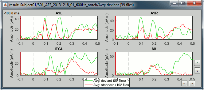
Now select the option "Overlay:Conditions", do not select "Overlay:Scouts", click on [Display].

In both conditions, we observe similar early responses (P50 and N100), then it diverges.
In the deviant condition, we observe a pattern A1-IFG-A1 that is absent in the standard conditions.Same scouts, deviant condition, Z-score. The signals are the same but scaled differently.
![[ATTACH] [ATTACH]](/moin_static1911/brainstorm1/img/attach.png)
From the database explorer
You have to display the sources on the cortex to create the scouts. But once they are created, you can directly display the scouts time series from the tree. It means that you can quickly compare the values for a scout between many different conditions without having to open them all.
- Close everything (toolbar button [X]).
Select the option "Overlay:Conditions", do not select "Overlay:Scouts".
Select the two average recordings in Run#01 folder > right-click > Scouts time series.
Note that this menu is present at all the levels in the database explorer.
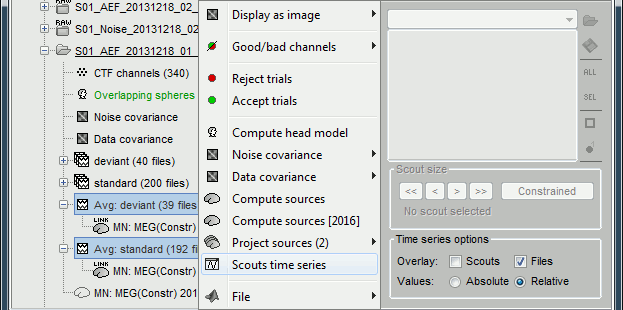
If no scout is currently loaded in the Scout tab, it shows all the scouts available in the surface.
If a surface is loaded, and at least one scout selected in the Scout tab, this popup menu would display only the selected scouts.
Unconstrained sources
Open any of the non-normalized source files in your database (average current density).
Select the option "Values: Relative", display the first scout in the list (A1L):
![[ATTACH] [ATTACH]](/moin_static1911/brainstorm1/img/attach.png)
It shows three graphs, corresponding to the three dipole orientations: A1L1=X, A1L2=Y, A1L3=Z
Scout toolbar and menus
Menu: Atlas
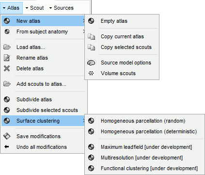
New atlas:
Empty atlas: Create a new empty atlas.
Copy atlas: Duplicates an atlas and all the scouts it contains.
Copy selected scouts: Create a new atlas and copy only the selected scouts to it.
Source model options: Create a special atlas "Source model", with which you can attribute different modeling constraints to each region. Create after merging the cortex with some subcortical regions. This is required to use the option "Custom head model" (mixed models).
Volume scouts: Create a volume atlas in order to store 3D scouts (volume head models).
Load atlas: Load ROIs or a cortical parcellation coming from FreeSurfer or BrainSuite as a new atlas.
Rename atlas: Change the name that appears in the atlas list to refer to the selected atlas.
Delete atlas: Delete the current atlas and all the scouts in contains.
Add scouts to atlas: Load ROIs or a cortical parcellation and add them to the current atlas.
Subdivide atlas: Splits all the scouts of the current atlas in smaller ROIs. Available options:
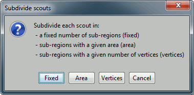
Subdivide selected scouts: Same thing, but processes only the selected scouts.
Surface clustering: Create a parcellation of the cortex surface and saves it as a new atlas.
Only the "Homogeneous parcellation" clustering is currently available.Save modifications: Force the current modifications to be saved to the cortex surface.
Undo all modifications: Restore the atlas the way it was the last time the surface was loaded.
Menu: Scout
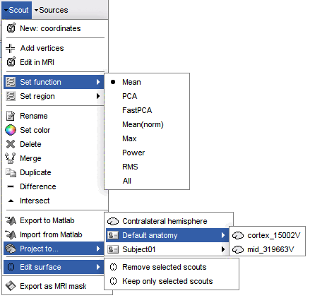
New: coordinates: Create a new scout starting from the vertex that is the closest to the specified coordinates. You can enter coordinates in MRI, SCS or MNI coordinates.
Add vertices: The user can select some points on the cortex surface and add them to the scout.
Equivalent: Click on Select point (first toolbar button) then select the scout in list.Edit in MRI: Open an interface to edit the select scout as a 3D ROI, slice by slice. Only the vertices contained in the 3D mask are kept, all the volume information is lost. It means that the mask you intendend to draw might be very different from what you get as a scout at the end. This is not a very reliable tool, as there is no direct correspondence between the volume and the surface.
Set function: Set the scout function for the selected scouts.
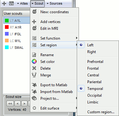
Set region: Set the cortical region for the selected scouts.
Rename: Rename the selected scout. Shortcut: double-click.
Set color: Change the display color of scout patch in 3D figures.
Delete: Delete selected scouts. Shortcut: Delete key
Merge: Join two or more selected scouts.
Export to Matlab: Export the structures of the selected scouts to the Matlab environment and makes them accessible from the command window. This menu can be useful to get quickly the list of vertex indices or modify a scout manually.
Import from Matlab: Import scouts structures that you modified manually from your Matlab command window directly as new scouts.
Project to: Project the selected scout on another surface available in the database.
Edit surface: Create a new surface containing only the desired parts (remove or keep only the selected scouts). This is useful for instance for selecting one sub-cortical region from the Aseg FreeSurfer atlas (see the FreeSurfer tutorial).
Menu: Sources
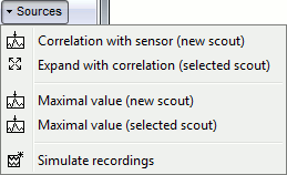
Correlation with sensor: Create a new scout with all the sources that are strongly correlated with a given sensor.
Expand with correlation: Computes the correlation between the values for the scout's seed (first point) and all the other sources. The sources that have correlation coefficient superior to a given threshold are added to the scout.
Maximal value (new scout): Find the vertex with the maximal intensity at the current time, and create a scout centered on it.
Maximal value (selected scout): Move the scout's seed to the source that has the maximum amplitude in the scout, at the current time.
Simulate recordings: Multiply the selected scouts with the forward model. Simulate the scalp data that would be recorded if only the selected cortex region was activated; all the other sources are set to zero. Create a new data file in the database.
If no scout selected: simulate recordings produced by the activity of the entire cortex.
Scout region
A scout is defined by its name, and it has several properties: a list of vertices and an aggregating function. These are usually enough to explore the activity at the cortex level the way we did it in these tutorials. An extra property can be defined on the scout: the explicit classification in a brain region. This property is used only in more advanced functional connectivity analysis, for the representation of the NxN connection graphs. It is introduced here for reference purpose.
A brain region in Brainstorm is following a hierarchy with three levels: hemisphere / lobe / sub-region. The definition at each level is optional: a region can be classified only at the hemisphere level, or at the hemisphere+lobe level, or none of them. It depends on level or hierarchy you are interested in to explore the connectivity graphs.
The region for a scout can be set with the Scout > Set region menus, and is encoded in a string that contains at least 2 characters: "HLxxx". H represents the hemisphere (L,R,U), L stands for the lobe (F,PF,C,P,T,O,L,U), and xxx for the sub-region name (optional). For both the hemisphere and the lobe, the value "U" stands for "Undefined", meaning that the classification is simply not set. The menu Set region>Custom region... lets you edit this string directly. The menu Set region>Undefined sets the region string to "UU" (undefined hemisphere, undefined lobe).
When set, the region string is shown before the scout name in the list, representing only the defined levels. It doesn't show the letters U for "undefined", therefore the scouts you create manually, that are by default set to "UU", do not show any extra string.
On the hard drive
The scouts are saved in the surface file on which they have been defined.
In the anatomy view, right-click on the selected cortex surface (cortex_15002V) > View file contents.
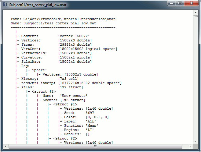
Fields in the surface files:


