|
Size: 27204
Comment:
|
Size: 29475
Comment:
|
| Deletions are marked like this. | Additions are marked like this. |
| Line 2: | Line 2: |
| ''Authors: Francois Tadel, Elizabeth Bock, Dimitrios Pantazis, Sylvain Baillet'' | ''Authors: Francois Tadel, Dimitrios Pantazis, Elizabeth Bock, Sylvain Baillet'' |
| Line 13: | Line 13: |
| In Brainstorm we offer two approaches for computing time-frequency decomposition (TF): the first one is based on the convolution of the signal with series of complex Morlet wavelets, the second filters the signal in different frequency bands and extract the envelope of the filtered signals using the Hilbert transform. | In Brainstorm we offer two approaches for computing time-frequency decomposition (TF): the first one is based on the convolution of the signal with series of complex Morlet wavelets, the second filters the signal in different frequency bands and extracts the envelope of the filtered signals using the Hilbert transform. |
| Line 28: | Line 28: |
| {{attachment:waveletOptions.gif||height="291px",width="637px"}} | {{attachment:waveletOptions.gif||width="650px"}} |
| Line 36: | Line 36: |
== Simulation == We will illustrate the time-frequency decomposition process with a simulated signal. * The following code generates a sum of three sinusoids (2Hz, 20Hz, 50Hz).<<BR>>The 50Hz is present everywhere, the two others start only after two seconds.<<BR>> {{{ f1 = 2; f2 = 20; f3 = 50; i =2000:6000; Data(1,i) = sin(f1*2*pi*t(i)) + 0.4 * cos(f2*2*pi*t(i)); Data = Data + 0.2 * sin(f3*2*pi*t); }}} * Empty the Process1 list (right-click > Clear list) then click on [Run]. * Select process: '''Simulate > Simulate genertic signals'''. <<BR>>Ntime='''6000''', Sampling frequency='''1000Hz''' (signal duration = 6000/1000 = 6 seconds).<<BR>>Copy-paste the few lines of code above to generate the sum of three sinusoids.<<BR>><<BR>> {{attachment:simulate_process.gif||height="412",width="489"}} * Double-click on the new file to look at the simulated signal.<<BR>><<BR>> {{attachment:simulate_display.gif||height="159",width="667"}} |
|
| Line 155: | Line 170: |
| * Note that if you right-click on the file in the '''database explorer''' and then select one of these menus, it will show '''all the sensors'''. If you right-click on an existing '''time-frequency figure''' with only one sensor displayed to get these menus, it will show only the '''selected sensor'''. | |
| Line 180: | Line 196: |
| * A better approach would have been to import longer epochs (+200ms on each side), then to normalize the values based on the "safe" part of the baseline (100ms-0ms). If you include the edge effects in your baseline, you end up propagating them in all the epoch. | |
| Line 184: | Line 201: |
| == Cortical sources | Hilbert transform == | == Cortical sources / Hilbert transform == |
| Line 199: | Line 216: |
| * '''Shift + click '''on the cortex surface: Displays the TF decomposition of the selected source.<<BR>>In the TF doesn't show as a high value because this the file that hasn't been normalized.<<BR>><<BR>> {{attachment:tf_sources.gif}} | * '''Shift + click '''on the cortex surface: Displays the TF decomposition of the selected source.<<BR>>In the TF figure, it doesn't show as a high value because this file hasn't been normalized.<<BR>><<BR>> {{attachment:tf_sources.gif}} |
| Line 209: | Line 226: |
| ==== Description of the fields ==== | ==== Structure of the time-frequency files: timefreq_*.mat ==== |
| Line 216: | Line 233: |
| * '''Freqs''': For regular frequency binning: vector containing all the frequencies.<<BR>> If using frequency bands: [Nfreqbands x 3] cell array, where each line represents a frequency band {'band_name', 'frequency definition', 'function'} |
* '''Freqs''': For regular frequency binning: vector containing all the frequencies.<<BR>>If using frequency bands: [Nfreqbands x 3] cell array, where each line represents a frequency band {'band_name', 'frequency definition', 'function'} |
| Line 237: | Line 252: |
| ==== Useful functions ==== * '''in_bst_timefreq'''(TimefreqFile): Read a time-frequency file. * '''in_bst'''(FileName, TimeWindow): Read any Brainstorm file with the possibility to load only a specific part of the file. "TimeWindow" is an range of time values in seconds: [tStart, tStop]. * '''bst_process'''(''''LoadInputFile'''', FileName, Target, TimeWindow): The most high-level function for reading data files. "Target" is a string with the list of sensor names or types to load. |
|
| Line 240: | Line 260: |
| == Delete all your experiments == Before moving to the next tutorial, '''delete '''all the time-frequency files you computed in this tutorial. It will make the database structure less confusing for the following tutorials. |
|
| Line 242: | Line 265: |
| <<EmbedContent("http://neuroimage.usc.edu/bst/get_prevnext.php?prev=Tutorials/Scouts&next=Tutorials/Statistics")>> | <<EmbedContent("http://neuroimage.usc.edu/bst/get_prevnext.php?prev=Tutorials/Scouts&next=Tutorials/Difference")>> |
Tutorial 24: Time-frequency
Authors: Francois Tadel, Dimitrios Pantazis, Elizabeth Bock, Sylvain Baillet
This tutorial introduces how to compute time-frequency decomposition of MEG/EEG recordings and cortical currents using complex Morlet wavelets and Hilbert transforms.
Contents
- Introduction
- Morlet wavelets
- Edge effects
- Simulation
- Simple example
- Process options
- Display: One channel
- Display: Mouse and keyboard shortcuts
- Display: All channels
- Display: Sensor topography
- Display: Power spectrum and time series
- Scouts / Single trials
- Normalized time-frequency maps
- Cortical sources / Hilbert transform
- On the hard drive
- Additional documentation
- Delete all your experiments
Introduction
Some of the MEG/EEG signal properties are difficult to access in time domain (graphs time/amplitude). A lot of the information of interest is carried by oscillations at certain frequencies, but the amplitude of these oscillations is sometimes a lot lower than the amplitude of the slower components of the signal, making them difficult to observe.
The averaging in time domain may also lead to a cancellation of these oscillations when they are not strictly locked in phase across trials. Averaging trials in time-frequency domain allows to extract the power of the oscillation regardless of the phase shifts. For a better understanding of this topic, we recommend the lecture of the following article: Bertrand O, Tallon-Baudry C (2000), Oscillatory gamma activity in humans: a possible role for object representation
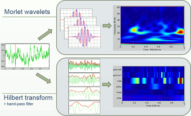
In Brainstorm we offer two approaches for computing time-frequency decomposition (TF): the first one is based on the convolution of the signal with series of complex Morlet wavelets, the second filters the signal in different frequency bands and extracts the envelope of the filtered signals using the Hilbert transform.
Morlet wavelets
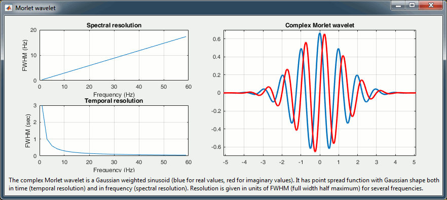
Complex Morlet wavelets are very popular in EEG/MEG data analysis for time-frequency decomposition. They have the shape of a sinusoid, weighted by a Gaussian kernel, and they can therefore capture local oscillatory components in the time series. An example of this wavelet is shown below, where the blue and red curves represent the real and imaginary part, respectively.
Contrary to the standard short-time Fourier transform, wavelets have variable resolution in time and frequency. When designing the wavelet, we basically decide a trade off between temporal and spectral resolution.
To design the wavelet, we first need to choose a central frequency, ie the frequency where we will define the mother wavelet. All other wavelets will be scaled and shifted versions of the mother wavelet. Unless interested in designing the wavelet at a particular frequency band, the default 1Hz should be fine.
Then, the desirable time resolution for the central frequency should be defined. For example, we may wish to have a temporal resolution of 3 seconds at frequency 1 Hz (default parameters). These two parameters, uniquely define the temporal and spectral resolution of the wavelet for all other frequencies, as shown in the plots below.
Resolution is given in units of Full Width Half Maximum of the Gaussian kernel, both in time and frequency. The relevant plots are given below.
Edge effects
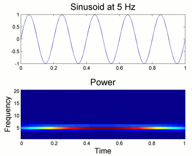
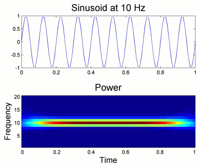
Users should pay attention to edge effects when applying wavelet analysis. Wavelet coefficients are computed by convolving the wavelet kernel with the time series. Similarly to any convolution of signals, there is zero padding at the edges of the time series and therefore the wavelet coefficients are weaker at the beginning and end of the time series.
From the figure above, which designs the Morlet wavelet, we can see that the default wavelet (central frequency 1Hz, FWHM=3sec) has temporal resolution 0.25sec at 5Hz and 0.1sec at 10Hz. In such case, the edge effects are roughly half these times: 125ms in 5Hz and 50ms in 10Hz. Examples of such edge effects are given in the figures below.
Simulation
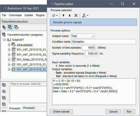
We will illustrate the time-frequency decomposition process with a simulated signal.
The following code generates a sum of three sinusoids (2Hz, 20Hz, 50Hz).
The 50Hz is present everywhere, the two others start only after two seconds.
f1 = 2; f2 = 20; f3 = 50;
i =2000:6000;
Data(1,i) = sin(f1*2*pi*t(i)) + 0.4 * cos(f2*2*pi*t(i));
Data = Data + 0.2 * sin(f3*2*pi*t);
Empty the Process1 list (right-click > Clear list) then click on [Run].
Select process: Simulate > Simulate genertic signals.
Ntime=6000, Sampling frequency=1000Hz (signal duration = 6000/1000 = 6 seconds).
Copy-paste the few lines of code above to generate the sum of three sinusoids.
Double-click on the new file to look at the simulated signal.

Simple example
Let's start with a simple example to explore the options of the time-frequency decomposition process.
In Process1, select the average recordings for the deviant condition for Run#01.
Select process: Frequency > Time-frequency (Morlet wavelets).
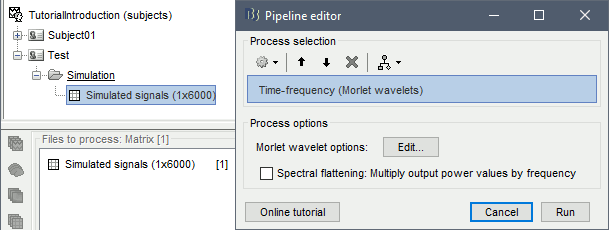
Enter "MEG" for the sensor types, do not select the "Spectral flattening" option.
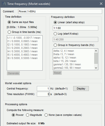
Click on the button [Edit] to see all the process options.
Time definition: Same as input, Frequency definition: Log 1:40:150, Compute measure: Power.
Note that in general, you should not compute the time-frequency decomposition of the average, but rather TF decomposition of the single trials and average the power of the TF maps you obtain.
This is illustrated in the section "Scouts / Single trials" below.
Process options
Comment: String that will be displayed in the database explorer to represent the output file.
Time definition
Same as input file: The output file has the same time definition as the input file.
In this example, it means: 361 samples between -100ms and 500ms.Group in time bands: This option adds a step of computation. First it computes the TF decomposition for all the input file, then averages the power by time band. To define a time band:
Enter your own time bands in the text area, one line per time band, with the following format: "name / time definition / function"
- Click on the button [Generate] to automatically create a list of time bands with the same length. You will be asked the maximal length of each time band.
The function is the measure we take to combine the values for all the individual frequencies into one for the frequency band. Possible values are: mean, max, std, median.
Frequency definition: Frequencies for which the power will be estimated at each time instant.
Linear: You can specify the frequencies with the Matlab syntax start:step:stop.
The default is "1:1:60", which produces 60 values [1, 2, 3, 4, ..., 59, 60].Group in frequency bands: As for the time definition, this option leads to a two-step process. First it computes the TF decomposition for several values in the frequency band, then it averages the power of TF coefficients per frequency band. To define a frequency band:
One line per frequency band, with the format "name / frequency definition / function"
The frequency definition is a Matlab expression evaluated with an eval() call. If the frequency definition contains only two values, Brainstorm adds two extra values in the middle so that the final averaged value is a bit more robust. Example of valid expressions:
"2,4": Evaluates to [2,4], and then expands to the frequency vector [2, 2.66, 3.33, 4]
"2:0.5:4": Evaluates to [2 2.5 3 3.5 4]
"2, 2.5, 3, 3.5, 4": Evaluates to [2 2.5 3 3.5 4]The function is the measure we take to combine the values for all the individual frequencies into one for the frequency band. Possible values are: mean, max, std, median.
Morlet wavelet options
Central frequency: Frequency where the mother wavelet is designed. All other wavelets will be shifted and scaled versions of the mother wavelet
Time resolution (FWHM): Temporal resolution of the wavelet at the central frequency (in units of Full Width Half Maximum). Click [Display] to see the resolution of the wavelet for other frequencies.
Compute the following measure:
- The convolution of the signal with complex Morlet wavelets returns the complex coefficients for each frequency/time/sensor. Typically, what we display is the power of the coefficients (square of the amplitude: abs(TF).^2). You can choose if you want to apply this transformation or not.
Power: Computes the "power" transformation immediately after the TF decomposition. This discards the phase information, but produces files that are twice smaller and a lot easier to process.
None: Save the TF coefficients as they are computed. This can be useful if you plan to use these decompositions for other purposes that require the phase.
- Some combinations of options may disable this choice. If you select frequency bands, the program will have to compute the power before averaging the values, therefore "none" is not an option.
Display: One channel
Right on the new time-frequency file > One channel (same as double-clicking on the file).

This menu displays the time-frequency decomposition of the first sensor. The Brainstorm window shows two new elements: the tab "Display" and the "current frequency" slider.
![[ATTACH] [ATTACH]](/moin_static198/brainstorm1/img/attach.png)
Current frequency: Slider that shows the current frequency selected in all the figures.
Just like the time, the frequency selection is centralized and managed by one control only for all the figures. As a consequence, it is impossible to display TF files with different frequency definitions at the same time. This can be perceived as an annoying limitation, but it allows all the simultaneous displays to be consistent at anytime and makes the interface more intuitive to manipulate, with lower risks of mistakes in the interpretation of the different figures.List of sensors: This drop-down list shows the current entry displayed in the selected figure. In this case, it is by default the MEG sensor "MLC11". Try to change it, it will update the display of the figure, showing the frequency power for another sensor.
Hide edge effects: When this option is selected, the time-frequency coefficients that could not be properly estimated because of a lack of time samples are hidden. It allows you to see only the information that is really reliable. In this example, you can see that it masks a large portion of the window: 600ms is not enough to perform a correct time-frequency decomposition. Try to work on much larger time windows when using these tools.
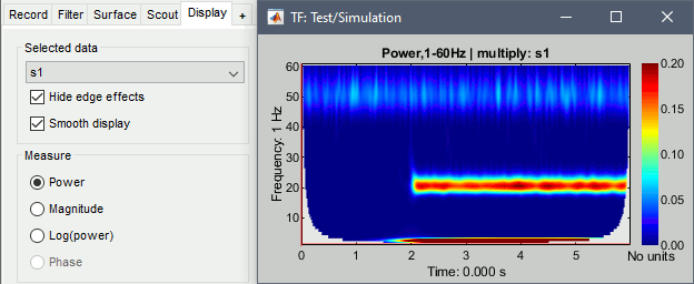
Smooth display: Re-interpolates the time-frequency maps on a finer grid to produce nicer plots.
Measure: Type of measure that is currently represented in the selected figure. The entries that are enabled depend on the type of data that is saved in the file. In this case, we saved directly the power of the wavelet coefficients in the file, we discarded the angle/phase information, so the "phase" option is disabled. The other options are: Magnitude = sqrt(power), Log = 10*log10(power)
Colormap: As explained in the previous tutorials, you can change the colormap by clicking+moving on the colorbar on the right of the figure. Double-click on the colorbar to restore the defaults.
Display: Mouse and keyboard shortcuts
Mouse shortcuts
Left-click: Selection of current time and frequency.
Left-click + move: Select a time/frequency range. The legends of the X/Y axis show the selection.
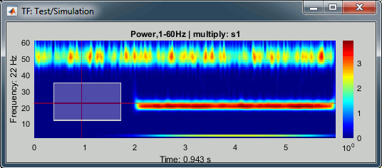
Mouse wheel: Zoom in time, centered on the current time cursor.
Control + mouse wheel: Zoom in frequencies, centered on the current frequency cursor.
Right-click + move, or Control + left-click + move: Move in the zoomed image.
Double-click: Restore initial view.
Keyboard shortcuts:
Left/right arrows: Change the current time.
Page-up/page-down: Change the current time, 10 time samples at a time.
Up/down arrows: Change the the sensor displayed in this figure.
Control + up/down arrows: Change the current frequency.
Enter: View the original time series for this sensor.
Control + R: View the original MEG recordings.
Control + T: View the time-frequency 2D topography.
Control + I: Save as image.
Control + D: Dock figure in the Matlab environment.
Figure popup menu
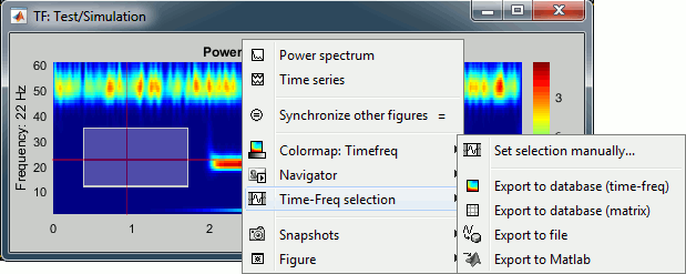
Set selection manually: Does the same thing as drawing a time/freq selection square on a figure, but by typing the values for time and frequency manually.
Export to database: Save the selection for the displayed sensor in a new file in the database.
Export to file: Same as "Export to database", but the saved file is not registered in the database.
Export to Matlab: Same as "Export to database", but the output structure is sent to a variable in the Matlab base workspace instead of being saved to a file.
Display: All channels
Three menus display the time-frequency of all the sensors with different spatial organizations.
All channels: All the maps are displayed one after the other, in the order they are saved in the file.
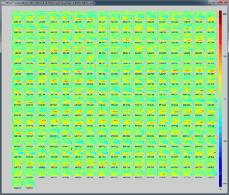
2D Layout (maps): Show each TF map where the sensor is located on a flattened 2D map.
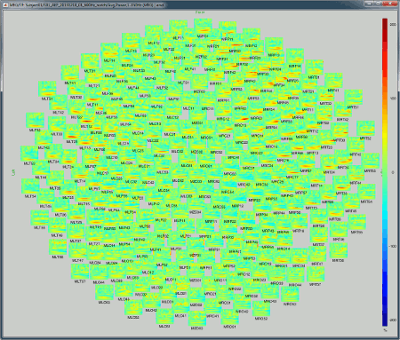
2D Layout (no overlap): Similar to the the previous display, but the positions of the images are reorganized so that they do not overlap.
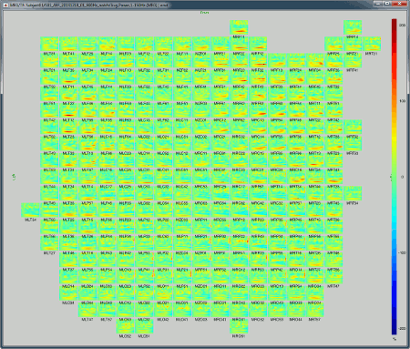
Useful shortcuts for these figures:
Click: clicking on any small TF image opens a new figure to display only the selected sensor.
Shift + click: Same, but opens the original recordings time series of the sensor instead of the TF.
Mouse wheel: Zoom in/out.
Right click + move: Move in a zoomed figure.
Display: Sensor topography
The menus below show the distribution of TF power over the sensors, for one time point and one frequency bin, very similarly to what was introduced in tutorial Visual exploration.
2D Sensor cap / 2D Disc / 3D Sensor cap: 90ms, 8Hz

2D Layout: 8Hz (black), 35Hz (white)
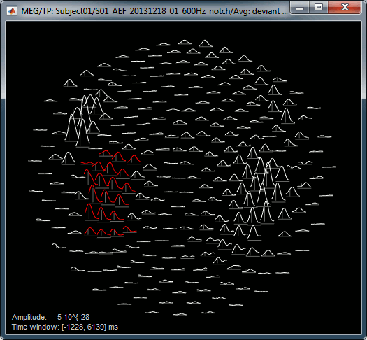
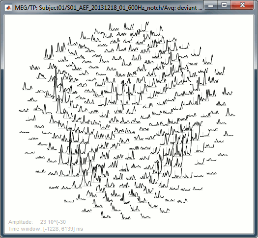
Useful shortcuts for these figures:
Left/right arrows: Change the current time.
Up/down arrows: Change the current frequency.
Control + E: Display the sensors markers/names.
Shift + click on a sensor: Displays the time-frequency decomposition for that specific sensors.
Right click + move: Select a group of sensors.
Shift + scroll: Change the gain of the time series (2D Layout).
Control + scroll: Change the length of the window displayed around the current time (2D Layout).
Display: Power spectrum and time series
These two menus generate similar figures:
Power spectrum: For the current time, shows the power of all the sensors across the frequencies.
Time series: For the current frequency, shows the power of all the sensors in time.
![[ATTACH] [ATTACH]](/moin_static198/brainstorm1/img/attach.png)
Note that if you right-click on the file in the database explorer and then select one of these menus, it will show all the sensors. If you right-click on an existing time-frequency figure with only one sensor displayed to get these menus, it will show only the selected sensor.
Scouts / Single trials
Similar calculations can be done at the level of the sources, either on the full cortex surface or on a limited number of regions of interests. We will start with the latter as it is usually an easier approach.
We will use this section to illustrate the online averaging of the trials TF decomposition as well.
Drag and drop all the deviant trials from both runs, select [Process sources].
Run process "Frequency > Time-frequency (Morlet wavelets)".
Select the option "Use scouts" and select all the scouts defined in the previous tutorial.
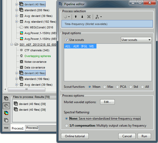
In the advanced options, select "Scout function: After" and "Output: Save average".
Run the process (it may take a while).
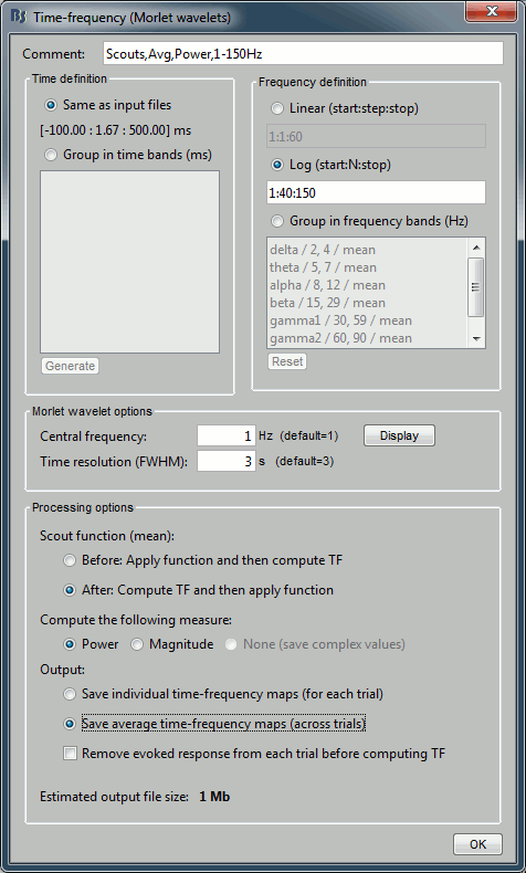
- The scout function was introduced in the previous tutorial. It is the method we use to group the time series for the 40*3=120 unconstrained dipoles we have in each scout into one unique signal per orientation (three signals in the unconstrained case). When computing the TF of one scout, we have the choice between applying this function before or after the time-frequency decomposition itself.
Before: Extract the 120 source signals, apply the scout function to get three signals (one per orientation), run the TF decomposition of the three signals, and finally sum the power of the three TF maps. This is faster but may lose some frequency resolution (especially for constrained sources).
After: Extract the 120 source signals, run the TF decomposition of the 120 signals, apply the scout function on the power of the TF maps for each orientation separately, and finally sum the three orientations. You should always prefer this option if the computation times are not insane.
Save individual TF maps: This option stops the computation here and saves in the database one time-frequency file for each input file (40 files), with one TF map for each scout.
Save average TF maps: Instead of saving the TF for each file separately, it automatically computes the average of the power of all the TF. This is a good choice if you do not plan to use independently all the TF files, because it saves a lot of time and disk space.
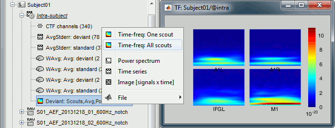
Rename the new file to add a tag "Deviant" in it. Then right-click > Time-freq: All scouts.
Normalized time-frequency maps
The brain is always active, the MEG/EEG recordings are never flat, some oscillations are always present in the signals. Therefore we are often more interested in the transient changes in the power at certain frequencies than at their amplitude. A good way to observe those changes is to compute a deviation of the power with respect with a baseline. This section illustrates the two methods Brainstorm offers to normalize the TF maps.
There is another reason for which we are usually interested in standardizing the TF values. The power of the time-frequency coefficients are always lower in the higher frequencies than in the lower frequencies, the signal carries a lot less power in the small and faster oscillations than in the slow brain responses. This 1/f decrease in power is an observation that we already made with the power spectrum density in the filtering tutorial.
If we represent the TF maps with a linear color scale, we will always see values close to zero in the higher frequency ranges. Normalizing each frequency separately with respect with a baseline helps obtaining more readable TF maps.
Drag and drop the new time-frequency file in Process1, select the "Time-frequency" button.
Run the process "Standardize > Z-score normalization", baseline [-100,-2]ms.
![[ATTACH] [ATTACH]](/moin_static198/brainstorm1/img/attach.png)
Run also the process "Standardize > Event-related perturbation (ERS/ERD)", [-100,-2]ms:
![[ATTACH] [ATTACH]](/moin_static198/brainstorm1/img/attach.png)
![[ATTACH] [ATTACH]](/moin_static198/brainstorm1/img/attach.png)
Double-click on the original TF file and the two normalized files (center=Z-score, right=ERD/ERS). Select the option "Smooth display" to make the figures look nicer.
![[ATTACH] [ATTACH]](/moin_static198/brainstorm1/img/attach.png)
The normalized maps seem to show a response of the left primary auditory cortex (A1L is the first scout in the file) around 35Hz and 80ms. The large red part at the lower frequency is probably part of the evoked response to the stimulus, but all those values could not be estimated properly because the time window is not long enough. Because we used the baseline between -100ms and 0ms, we cannot really trust anything below 30Hz or 40Hz.
![[ATTACH] [ATTACH]](/moin_static198/brainstorm1/img/attach.png)
- A better approach would have been to import longer epochs (+200ms on each side), then to normalize the values based on the "safe" part of the baseline (100ms-0ms). If you include the edge effects in your baseline, you end up propagating them in all the epoch.
The figures do not use the same colormaps because the original TF file is displayed using the colormap "Timefreq" while the normalized files are displayed using the colormap "Stat 2". If you want to look at the normalized maps using a different colormap, right-click on the figure and change the colormap configuration.
Cortical sources / Hilbert transform
Computing the time-frequency decomposition for all the sources of the cortex surface is possible but complicated because it can easily generate gigantic files, completely out of the reach of most computers. For instance the full TF matrix for each epoch we have here would be [Nsources x Ntimes x Nfrequencies] = [45000 x 361 x 40] double-complex = 9.7 Gb!
We have two ways of going around this issue: computing the TF decomposition for fewer frequency bins or frequency bands at a time, or computing the TF decomposition of the sensor values and projecting it dynamically to the cortex using the inverse operator.
This latter approach is possible because the two processes (TF decomposition and inversion) are linear and permutable. However this is enabled only for contrained sources (so not possible in the present case).
TF(Inverse(Recordings)) = Inverse(TF(Recordings))
=> Power(TF(Inverse(Recordings))) = Power(Inverse(TF(Recordings)))
For illustration purpose, we will use the other time-frequency decomposition option available in Brainstorm, which is based on Hilbert transforms of band-passed signals, using only 6 pre-defined frequency bands.
Drag and drop in Process1 the sources for the deviant average in Run#01.
Select the process "Frequency > Hilbert transform".
To process the entire brain, do not select the option "Use scouts".
![[ATTACH] [ATTACH]](/moin_static198/brainstorm1/img/attach.png)
In the advanced options, select "No, save full hilbert(sources)" because the other option is not available on unconstrained sources, and "magnitude" to divide the size of the file by two.
![[ATTACH] [ATTACH]](/moin_static198/brainstorm1/img/attach.png)
The frequency slider now shows frequency bands ("alpha:8-12Hz") instead of frequencies ("12Hz").
At 90ms, we observe a strong response in the auditory cortex in the alpha band (left) and a response in the motor cortex in the low gamma (right).
This could make sense, but this is for illustration purpose only, as we said before we cannot interpret what is happening at 10Hz, and we shouldn't have been computing the decomposition of the average, but rather the average of the TF of all the trials.
![[ATTACH] [ATTACH]](/moin_static198/brainstorm1/img/attach.png)
![[ATTACH] [ATTACH]](/moin_static198/brainstorm1/img/attach.png)
Shift + click on the cortex surface: Displays the TF decomposition of the selected source.
In the TF figure, it doesn't show as a high value because this file hasn't been normalized.
![[ATTACH] [ATTACH]](/moin_static198/brainstorm1/img/attach.png)
Right-click on the brain: Selects the closest vertex and displays the popup menu at the same time. The first three menus are relative to the source that was just clicked.
![[ATTACH] [ATTACH]](/moin_static198/brainstorm1/img/attach.png)
On the hard drive
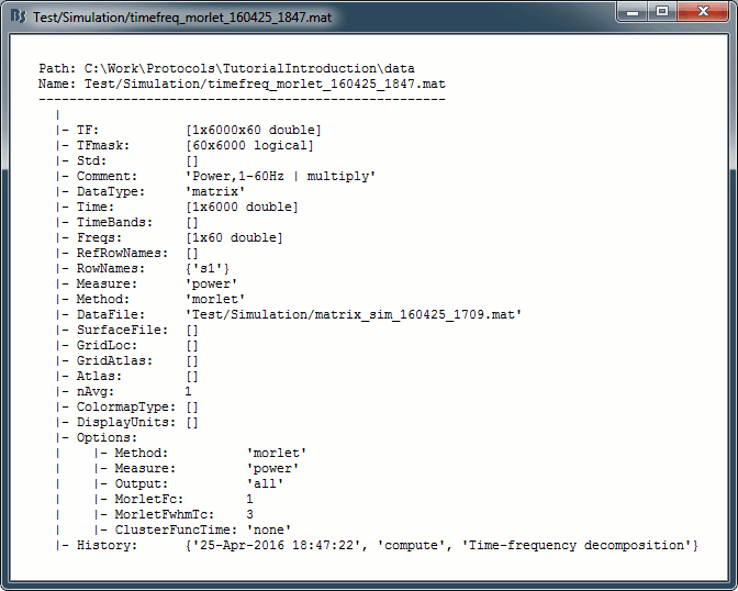
Right click one of the first TF file we computed > File > View file contents.
Structure of the time-frequency files: timefreq_*.mat
TF: [Nsignals x Ntime x Nfrequencies] matrix containing all the values of the time-frequency decomposition (complex wavelet coefficients, or double values for power/magnitude/Z-score).
Std: [Nsignals x Ntime x Nfrequencies] standard deviation if this file is an average.
Comment: String displayed in the database explorer to represent the file.
DataType: From what kind of data this file was computed: {'data', 'results', 'scout, 'matrix'}
Time: [1 x Ntime] Time vector used to estimate this file.
TimeBands: [Ntimebands x 3] Cell array where each line represents a time band:
{'band_name', 'time definition', 'function'}Freqs: For regular frequency binning: vector containing all the frequencies.
If using frequency bands: [Nfreqbands x 3] cell array, where each line represents a frequency band {'band_name', 'frequency definition', 'function'}RefRowNames: Used only for connectivity matrices.
RowNames: [1 x Nsignals] Cell array of strings that describes each row of the TF matrix. In this specific case, it would be the list of all the MEG sensor names. But it could also be a list of names of scouts or clusters.
Measure: Contains the name of the function that was applied right after the computation of the wavelet coefficients. So it represents the type of data contained in the TF matrix. Possible values:
none: No measure applied, TF contains the complex wavelet coefficients.
power: Power for each frequency, ie. the square of the amplitude: abs(coefficients).^2
magnitude: abs(coefficients)
log: 10 * log10( abs(coefficients).^2)
phase: angle(coefficients)
Method: String that identifies the process that generated the file:
{'morlet', 'fft', 'psd', 'hilbert', 'corr', 'cohere', 'granger', 'plv'}DataFile: Initial file from which this file was computed. In the database explorer, the TF file will be shown as a child of this DataFile file.
SurfaceFile / GridLoc / GridAtlas: Source space that was used, only for source files.
nAvg: Number of trials that were averaged to obtain this file.
ColormapType: String, force a specific colormap type to be used when displaying this file.
DisplayUnits: String, force to use specific units when displaying this file.
Options: Options that were selected in the time-frequency options window.
History: List of operations performed on this file (menu File > View file history).
Useful functions
in_bst_timefreq(TimefreqFile): Read a time-frequency file.
in_bst(FileName, TimeWindow): Read any Brainstorm file with the possibility to load only a specific part of the file. "TimeWindow" is an range of time values in seconds: [tStart, tStop].
bst_process('LoadInputFile', FileName, Target, TimeWindow): The most high-level function for reading data files. "Target" is a string with the list of sensor names or types to load.
Additional documentation
Forum: Time and frequency resolution: http://neuroimage.usc.edu/forums/showthread.php?1848
Delete all your experiments
Before moving to the next tutorial, delete all the time-frequency files you computed in this tutorial. It will make the database structure less confusing for the following tutorials.

