|
Size: 6026
Comment:
|
Size: 10647
Comment: Updates to Dipole Information
|
| Deletions are marked like this. | Additions are marked like this. |
| Line 1: | Line 1: |
| = Computing and displaying dipoles = | = Scanning and displaying dipoles = ''Authors: Elizabeth Bock, Francois Tadel, John C Mosher'' In Brainstorm, the brain activity is typically estimated with distributed source models including thousands of dipoles, and represented as cortical maps or functional overlays on the MRI. Another common way of representing the source activity is to consider there is only one single active dipole that can explain most of the MEG/EEG recordings. We offer two options to estimate the position and orientation of the most significant dipole at each time point: a '''dipole scanning''' method, which selects the most significant dipole in a grid of dipoles that are already estimated, and a non-linear '''dipole fitting''' method, which searches iteratively for the dipole that explains the best the recordings. The former is described on this page, the latter in another tutorial: [[http://neuroimage.usc.edu/brainstorm/Tutorials/DipoleFitting|FieldTrip dipole fitting]]. |
| Line 4: | Line 10: |
| == Computing sources using the GLS == This process allows for a systematic scanning of sources using performance measures to display single dipoles. For this tutorial we will use the Generalized Least Squares (GLS) source modeling available in Brainstorm. |
== Dipole modeling == The example below uses the protocol TutorialIntroduction created in the [[http://neuroimage.usc.edu/brainstorm/Tutorials#Get_started|introduction tutorials]]. |
| Line 7: | Line 13: |
| 1. Select the protocol ''TutorialCTF''. Right-click on ''Subject01 / Left / ERF'' > ''Compute sources''. 1. In this window, you should select ''Expert Mode''. You will see the following menu. Select ''[Test] Mosher GLS''. Click OK. Use the default settings in the next menu and click OK.<<BR>><<BR>> {{attachment:compute_GLS.png||height="450",width="279"}} --- {{attachment:compute_GLS_options.png||height="593",width="289"}} 1. Two results were added under the ERF: GLS and GLS-P.<<BR>><<BR>> {{attachment:tree_display_GLSP.png||height="188",width="279"}} * '''GLS''': * '''GLS-P''': |
* Select the protocol TutorialIntroduction. Go to the view "Functional data (sorted by subjects)". * In the imported Run01, right-click on the head model > '''Compute sources 2016''' > '''Dipole modeling''' <<BR>><<BR>> {{attachment:compute_sources.gif||height="298",width="425"}} * This option is not a distributed source model like the minimum norm, that inverts the head model and explains all recordings with all the sources at once. It represents the performance of each individual dipole, ie. its ability to explain all the recordings at one time sample on its own. * At each point of the grid, '''three dipoles''' with orthogonal directions (x,y,z) are considered, just like the unconstrained minimum norm results. * You can display this result in the same way as the minimum norm solutions, but you have to be cautious with the interpretation of the figure. The value at each point does not indicate a current density but the ability of the corresponding dipole to explain all the recordings. The highest values indicate the best fitting dipoles. If you see two regions with high values, it doesn't mean that there are two sources but that if there was one source only, it could be located in either of these regions. * Open the new dipole model file for the standard condition, and go to '''100ms'''. We expect two sources to be activated (left and right auditory cortices), but we observe high dipole performances only in the left hemisphere, while the distributed minimum norm solution was detecting correctly the bilateral activity. The response on the left side being much higher in amplitude than the right one, the dipoles one the left are better capable of explaining all the recordings on their own. <<BR>><<BR>> {{attachment:dipmap_100ms.gif||height="168",width="676"}} * For more information about the impossibility to represent multiple sources with a single dipole, you can refer to the tutorial [[http://neuroimage.usc.edu/brainstorm/Tutorials/DipoleFitting#Multiple_dipoles|FieldTrip dipole fitting]]. We will keep on working with this example to illustrate the dipole scanning process, but we need to keep in mind that it will not be able to explain our recordings properly. * For a more meaningful example, refer to the tutorial [[http://neuroimage.usc.edu/brainstorm/Tutorials/Epilepsy#Dipole_scanning|EEG and epilepsy]]. |
| Line 13: | Line 22: |
| == Dipole Scanning == For this tutorial we will do the scanning on the GLS results. However, the dipole scanning is also available for sources computed with minimum norm Z-scored (i.e. MN MEG(Constr) | zscored), dSPM and sLORETA. |
== Dipole scanning == The process '''Sources > Dipole scanning''' searches the grid of dipoles computed previously for the most significant location. The information from the three orientations (x,y,z) are combined to get the optimal orientation at the best location. |
| Line 16: | Line 25: |
| 1. Drag and drop the GLS-P link into the Process 1 box. Click ''Run > Sources > Dipole scanning''.<<BR>><<BR>> {{attachment:process_box_GLSP.png||height="465",width="300"}} --- {{attachment:select_process_dipolescanning.png||height="262",width="250"}} 1. Use the defaults options: * '''Time Window''': This is the window over which the scanning will occur. The default option is to use the entire epoch. * '''Time between dipoles''': This allows you to change the resolution of the scanning. To use all time points, enter a 0 (default).<<BR>><<BR>> {{attachment:dipole_scanning_options.png||height="250",width="325"}} 1. The resulting dipole file is added under the Left condition.<<BR>><<BR>> {{attachment:tree_display_dipolefile.png||height="200",width="260"}} |
* In Process1, select the dipole model file for the standard condition. * Run process '''Sources > Dipoles scanning''': Time window='''[60,100]ms''' <<BR>><<BR>> {{attachment:process_scanning.gif||height="251",width="491"}} * Double-click on the file to open it. For help on how to manipulate this view, see [[http://neuroimage.usc.edu/brainstorm/Tutorials/ExploreAnatomy#MRI_in_3D|this tutorial]]. <<BR>>The process selected the most significant dipole at each time sample in the selected time window (60ms-100ms). <<BR>><<BR>> {{attachment:display_all.gif||height="275",width="659"}} |
| Line 22: | Line 29: |
| == Displaying Dipoles == 1. Right-click ''ERF|GLSP-dipole-scan > Display on cortex''. The ''Dipoles'' panel is now open and dipoles are displayed on the cortex. You can now explore the results using the options in the ''Dipoles'' panel:<<BR>><<BR>> {{attachment:dipole_panel.png||height="420",width="300"}} * Data options: filter the available dipoles according the specific measurement. For the GLSP, these are defined as: * '''Z-score''': * '''Goodness''': * '''Chi-square''': * '''Reduced Chi-square''': * '''Confvolume''': * Display options: these options allow for adjusting how the selected dipoles (according to the Data options) are displayed * '''Show max goodness''': will show the dipole with the maximum goodness (within the constraints of the ''Data options'') at the time point selected. If ''Show all time'' is selected, then this represents the maximum goodness over all time points. * '''Show all time''': plots all selected dipoles at all time points. Un-selecting this options will show only the current time point. * '''3D - Color dipoles according to Time''', Goodness of Fit, Z-score, Group: adjusts the colormap to reflect the measure. 1. In the Dipoles panel, select ''Show max goodness of fit'', ''Show all time'', and color the dipoles according to ''Goodness of Fit''. You should see the following display. Explore the panel options to familiarize yourself with the capabilities.<<BR>><<BR>> {{attachment:max_GOF_cortex.png||height="200",width="260"}} |
== Displaying dipoles == We have 25 dipoles saved in this file, one per time sample between 60ms and 100ms. You can use the Dipoles tab to display only the most significant dipoles, and change the way they are colored. |
| Line 36: | Line 32: |
| === Additional Example === Dipole scanning can also be restricted to a scout. In this example, the scanning is restricted to a scout named '2' and colored according to ''Goodness of Fit''<<BR>><<BR>> |
* Filter dipoles: * '''Goodness of fit''': Select the dipoles with a goodness of fit above the threshold. * '''ConfVol''': Select the dipoles with a confidence volume below the threshold (for Neuromag Xfit). * '''Chi-sqr''': Select the dipoles with a fitting error below the threshold (least squares). |
| Line 39: | Line 37: |
| {{attachment:scanning_options_scouts.png||height="200",width="204"}} --- {{attachment:scan_dipoles_on_scout.png||height="250",width="285"}} | * Display filters: * '''Show max goodness of fit''': Select only the dipole with the highest goodness of fit (among the dipoles matching the other selection filters). * '''Show all times''': Select the dipoles from all the time samples. Otherwise only the dipole corresponding to the current time is displayed (if it matches the other selection filters). * Color dipoles according to: * '''Time''': The color codes for the time sample at which the dipole was estimated (mostly useful when the option "show all times" is selected). Blue dipoles correspond to the beginning of the time window we scanned (60ms in this example), and red values to the end (100ms). * '''Goodness of fit''': The color codes for the goodness of fit, in percent between 0 and 100. * '''Group''': When multiple groups of dipoles are available in the file, all the dipoles from the same group would be displayed with the same color. This applies to dipoles estimated with Neuromag Xfit, or for dipole files that were [[http://neuroimage.usc.edu/brainstorm/Tutorials/DipoleFitting#Merging_dipole_files|merged together]]. |
| Line 41: | Line 45: |
| == Dipole models from Neuromag's Xfit and CTF's DipoleFit == Brainstorm can import dipoles that have been generated using external software: |
* Click on a dipole to get detailed information about its position, amplitude and significance. |
| Line 44: | Line 47: |
| '''Neuromag Source Modelling module, xfit:''' The .bdip format is described in [[attachment:bdip_format.pdf]]. For more information about xfit and the bdip format see Neuromag Software Manuals. | . {{attachment:dipole_infos.gif}} |
| Line 46: | Line 49: |
| '''CTF !DipoleFit:''' The !DipoleFit software and the .dip format is described in the CTF Software Manuals. | == Dipole information [Substantially edited] == Description of the measures displayed in the "Dipole info" window: |
| Line 48: | Line 52: |
| '''To import''' | * '''Performance''':The square root of "chi-squared" in the degrees of freedom. In the example, 46^(2)^ is the chi-square measure, in three degrees of freedom. Generally should be treated like z-scoring, since we typically only care about the one degree of orientation, thus any performance measure substantially greater than 5 may be thought of as "signficant." * '''Goodness''':The percent "goodness of fit," as in what percentage of the total variance is explained by the model variance. * '''Conf volume''': Only on Neuromag Xfit, which is passed to this display. Volume of error, expressed in cubic mm. * '''Amplitude''': Dipole strength along the three Cartesian directions (x,y,z), expressed in A-m. * '''Orientation''': Normalized orientation of the dipole expressed in Cartesian directions (x,y,z). * '''Intensity''': Norm of the three amplitudes: sqrt(Amplitude_x^2^ + Amplitude_y^2^ + Amplitude_z^2^), typically expressed in nA-m. * '''Chi-square''':The sum-square of the whitened residual, i.e. a measure of modeling error. If the noise covariance is properly expressed and the model is accurate, then the residual is chi-square distributed in the degrees of freedom. * '''DOF''': Degrees of freedom = number of sensors - 3. * '''Reduced Chi-square''': Chi-square / DOF. A convenient approximation to modeling error. A perfect fit and perfect noise will have a reduced chi-square of 1.0. For high DOF, theory suggests that a reduced chi-square > 1.2 represents modeling error. In practice, we find that reduced chi-square below 2 is acceptable, and that when the model is particularly wrong, reduced chi-square is substantially greater. |
| Line 50: | Line 62: |
| 1. Select the study where you want to import the dipole file 1. Right click and select ‘Import dipoles’ (Figure 1) 1. For Neuromag, you will be prompted to specify the number of subsets used for dipole fitting. '''In most cases, this will be one.''' If subsets are used, as defined in the text file $HOME/.meg_analysis/xfit_selections, then the number of subsets used needs to be input when prompted. (Figure 2)<<BR>><<BR>> |
== Neuromag Xfit and CTF DipoleFit == Brainstorm can import dipole files that have been generated using external software: |
| Line 54: | Line 65: |
| {{attachment:import.png||height="455",width="294"}} <<BR>><<BR>> Figure 1. Importing dipoles<<BR>><<BR>> {{attachment:dipoles_subsets_dialog.jpg}} <<BR>><<BR>> Figure 2. Neuromag option for channel subsets<<BR>><<BR>> | * '''Elekta-Neuromag'''''' Xfit:''' The .bdip format is described in the Neuromag software manuals. * '''CTF DipoleFit:''' The DipoleFit software and the .dip format are described in the CTF manuals. ==== Importing a dipole file ==== * Right-click on the folder where you want to import the dipole file > '''Import dipoles'''. <<BR>><<BR>> {{attachment:import_popup.gif}} * For Elekta-Neuromag .bdip files, you will be prompted to specify the number of subsets used for dipole fitting. '''In most cases, this will be 1.''' If subsets are used, as defined in the text file $HOME/.meg_analysis/xfit_selections, then the number of subsets used needs to be input when prompted. <<BR>><<BR>> {{attachment:dipoles_subsets_dialog.jpg}} |
| Line 58: | Line 74: |
| * Clicking on a subset will select all Groups with that subset. For example, selecting Subset #1 will select Group #1 (1), Group #2 (2), Group #3 (3), etc. | * Clicking on a subset will select all Groups with that subset. For example, selecting Subset #1 will select Group #1 (1), Group #2 (1), Group #3 (1), etc. |
| Line 60: | Line 76: |
| === Examples === * '''Example 1''' shows 5 subsets (channel groups of Left, Right, Anterior, Posterior, All Channels). When subset #2 is selected, dipoles fitted to the right channels are displayed. In this case, ''Show all time'' is selected for the 4 Groups (events) and colored according to ''Goodness of Fit''<<BR>><<BR>> |
==== Examples ==== * '''Example 1''': 5 subsets (channel groups of Left, Right, Anterior, Posterior, All Channels). When subset #2 is selected, dipoles fitted to the right channels are displayed. In this case, ''Show all time'' is selected for the 4 Groups (events) and colored according to ''Goodness of Fit''<<BR>><<BR>> {{attachment:subset_group_GOF.png||height="354",width="300"}} |
| Line 63: | Line 79: |
| {{attachment:subset_group_GOF.png||height="354",width="300"}} | * '''Example 2''': All groups and subsets at one time point (0.3 ms), with goodness of fit greater than 80%, colored according to ''Group''.<<BR>><<BR>> {{attachment:allgroups_allsubsets_1time.png||height="366",width="300"}} |
| Line 65: | Line 81: |
| * '''Example 2''' shows all groups and subsets at one time point (0.3 ms), with goodness of fit greater than 80%, colored according to ''Group''.<<BR>><<BR>> | == Additional documentation == * Tutorial: [[http://neuroimage.usc.edu/brainstorm/Tutorials/Epilepsy#Dipole_scanning|EEG and epilepsy: Dipole scanning]] * Tutorial: [[http://neuroimage.usc.edu/brainstorm/Tutorials/DipoleFitting|Dipoles: FieldTrip dipole fitting]] * Tutorial: [[http://neuroimage.usc.edu/brainstorm/Tutorials/PhantomElekta#Dipole_source_estimation|MEG current phantom (Elekta-Neuromag)]] * Tutorial: [[http://neuroimage.usc.edu/brainstorm/Tutorials/PhantomCtf#Dipole_scanning|MEG current phantom (CTF)]] * Tutorial: [[http://neuroimage.usc.edu/brainstorm/Tutorials/SourceEstimation|Source estimation]] |
| Line 67: | Line 88: |
| {{attachment:allgroups_allsubsets_1time.png||height="366",width="300"}} | <<EmbedContent(http://neuroimage.usc.edu/bst/get_feedback.php?Tutorials/TutDipScan)>> |
Scanning and displaying dipoles
Authors: Elizabeth Bock, Francois Tadel, John C Mosher
In Brainstorm, the brain activity is typically estimated with distributed source models including thousands of dipoles, and represented as cortical maps or functional overlays on the MRI. Another common way of representing the source activity is to consider there is only one single active dipole that can explain most of the MEG/EEG recordings.
We offer two options to estimate the position and orientation of the most significant dipole at each time point: a dipole scanning method, which selects the most significant dipole in a grid of dipoles that are already estimated, and a non-linear dipole fitting method, which searches iteratively for the dipole that explains the best the recordings. The former is described on this page, the latter in another tutorial: FieldTrip dipole fitting.
Contents
Dipole modeling
The example below uses the protocol TutorialIntroduction created in the introduction tutorials.
Select the protocol TutorialIntroduction. Go to the view "Functional data (sorted by subjects)".
In the imported Run01, right-click on the head model > Compute sources 2016 > Dipole modeling
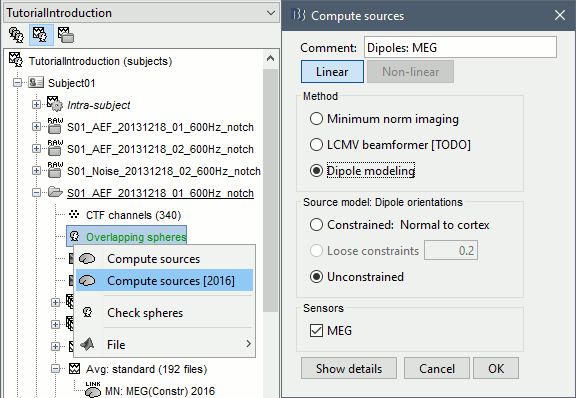
- This option is not a distributed source model like the minimum norm, that inverts the head model and explains all recordings with all the sources at once. It represents the performance of each individual dipole, ie. its ability to explain all the recordings at one time sample on its own.
At each point of the grid, three dipoles with orthogonal directions (x,y,z) are considered, just like the unconstrained minimum norm results.
- You can display this result in the same way as the minimum norm solutions, but you have to be cautious with the interpretation of the figure. The value at each point does not indicate a current density but the ability of the corresponding dipole to explain all the recordings. The highest values indicate the best fitting dipoles. If you see two regions with high values, it doesn't mean that there are two sources but that if there was one source only, it could be located in either of these regions.
Open the new dipole model file for the standard condition, and go to 100ms. We expect two sources to be activated (left and right auditory cortices), but we observe high dipole performances only in the left hemisphere, while the distributed minimum norm solution was detecting correctly the bilateral activity. The response on the left side being much higher in amplitude than the right one, the dipoles one the left are better capable of explaining all the recordings on their own.

For more information about the impossibility to represent multiple sources with a single dipole, you can refer to the tutorial FieldTrip dipole fitting. We will keep on working with this example to illustrate the dipole scanning process, but we need to keep in mind that it will not be able to explain our recordings properly.
For a more meaningful example, refer to the tutorial EEG and epilepsy.
Dipole scanning
The process Sources > Dipole scanning searches the grid of dipoles computed previously for the most significant location. The information from the three orientations (x,y,z) are combined to get the optimal orientation at the best location.
- In Process1, select the dipole model file for the standard condition.
Run process Sources > Dipoles scanning: Time window=[60,100]ms
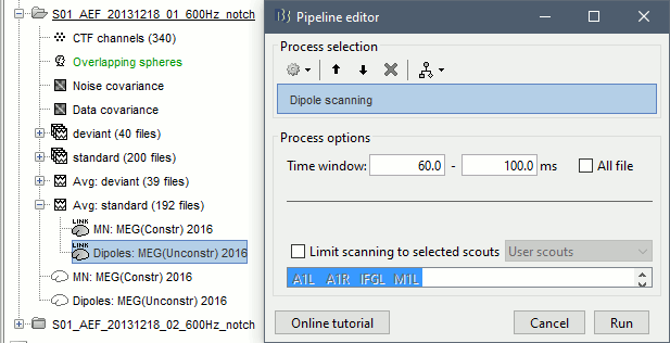
Double-click on the file to open it. For help on how to manipulate this view, see this tutorial.
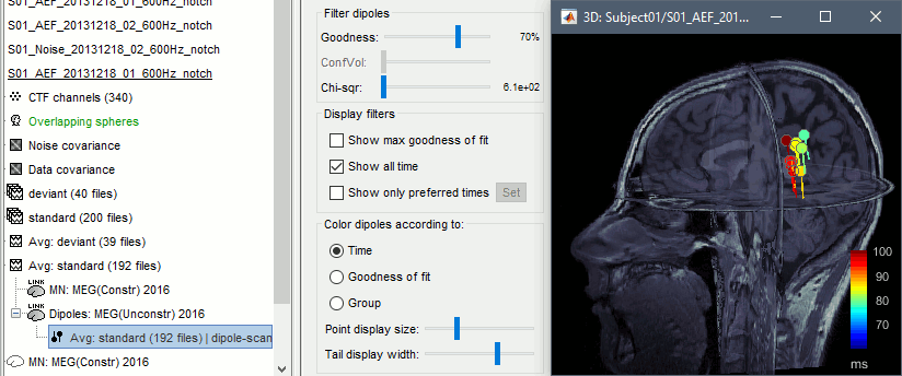
The process selected the most significant dipole at each time sample in the selected time window (60ms-100ms).
Displaying dipoles
We have 25 dipoles saved in this file, one per time sample between 60ms and 100ms. You can use the Dipoles tab to display only the most significant dipoles, and change the way they are colored.
- Filter dipoles:
Goodness of fit: Select the dipoles with a goodness of fit above the threshold.
ConfVol: Select the dipoles with a confidence volume below the threshold (for Neuromag Xfit).
Chi-sqr: Select the dipoles with a fitting error below the threshold (least squares).
- Display filters:
Show max goodness of fit: Select only the dipole with the highest goodness of fit (among the dipoles matching the other selection filters).
Show all times: Select the dipoles from all the time samples. Otherwise only the dipole corresponding to the current time is displayed (if it matches the other selection filters).
- Color dipoles according to:
Time: The color codes for the time sample at which the dipole was estimated (mostly useful when the option "show all times" is selected). Blue dipoles correspond to the beginning of the time window we scanned (60ms in this example), and red values to the end (100ms).
Goodness of fit: The color codes for the goodness of fit, in percent between 0 and 100.
Group: When multiple groups of dipoles are available in the file, all the dipoles from the same group would be displayed with the same color. This applies to dipoles estimated with Neuromag Xfit, or for dipole files that were merged together.
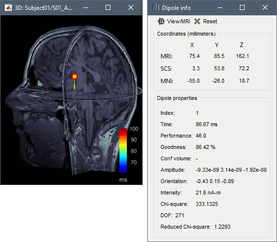
- Click on a dipole to get detailed information about its position, amplitude and significance.
Dipole information [Substantially edited]
Description of the measures displayed in the "Dipole info" window:
Performance:The square root of "chi-squared" in the degrees of freedom. In the example, 46(2) is the chi-square measure, in three degrees of freedom. Generally should be treated like z-scoring, since we typically only care about the one degree of orientation, thus any performance measure substantially greater than 5 may be thought of as "signficant."
Goodness:The percent "goodness of fit," as in what percentage of the total variance is explained by the model variance.
Conf volume: Only on Neuromag Xfit, which is passed to this display. Volume of error, expressed in cubic mm.
Amplitude: Dipole strength along the three Cartesian directions (x,y,z), expressed in A-m.
Orientation: Normalized orientation of the dipole expressed in Cartesian directions (x,y,z).
Intensity: Norm of the three amplitudes: sqrt(Amplitude_x2 + Amplitude_y2 + Amplitude_z2), typically expressed in nA-m.
Chi-square:The sum-square of the whitened residual, i.e. a measure of modeling error. If the noise covariance is properly expressed and the model is accurate, then the residual is chi-square distributed in the degrees of freedom.
DOF: Degrees of freedom = number of sensors - 3.
Reduced Chi-square: Chi-square / DOF. A convenient approximation to modeling error. A perfect fit and perfect noise will have a reduced chi-square of 1.0. For high DOF, theory suggests that a reduced chi-square > 1.2 represents modeling error. In practice, we find that reduced chi-square below 2 is acceptable, and that when the model is particularly wrong, reduced chi-square is substantially greater.
Neuromag Xfit and CTF DipoleFit
Brainstorm can import dipole files that have been generated using external software:
Elekta-Neuromag Xfit: The .bdip format is described in the Neuromag software manuals.
CTF DipoleFit: The DipoleFit software and the .dip format are described in the CTF manuals.
Importing a dipole file
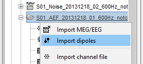
Right-click on the folder where you want to import the dipole file > Import dipoles.
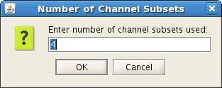
For Elekta-Neuromag .bdip files, you will be prompted to specify the number of subsets used for dipole fitting. In most cases, this will be 1. If subsets are used, as defined in the text file $HOME/.meg_analysis/xfit_selections, then the number of subsets used needs to be input when prompted.
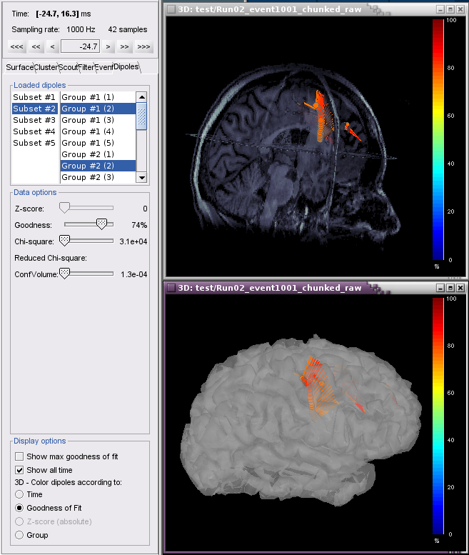
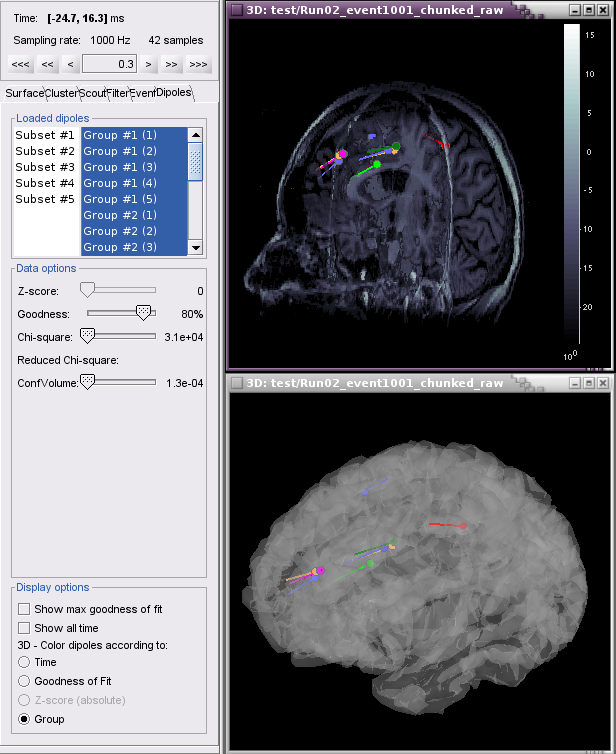
When displaying dipole files with multiple groups and/or subsets, the Loaded dipoles panel appears with a list of dipoles, grouped according to event (Group #1, Group#2, etc) and by channel subset, if used (Subset #1, Subset#2, etc.)
- Select the Group(s) to plot
- Clicking on a subset will select all Groups with that subset. For example, selecting Subset #1 will select Group #1 (1), Group #2 (1), Group #3 (1), etc.
Examples
Example 1: 5 subsets (channel groups of Left, Right, Anterior, Posterior, All Channels). When subset #2 is selected, dipoles fitted to the right channels are displayed. In this case, Show all time is selected for the 4 Groups (events) and colored according to Goodness of Fit
Example 2: All groups and subsets at one time point (0.3 ms), with goodness of fit greater than 80%, colored according to Group.
Additional documentation
Tutorial: EEG and epilepsy: Dipole scanning
Tutorial: Dipoles: FieldTrip dipole fitting
Tutorial: MEG current phantom (Elekta-Neuromag)
Tutorial: MEG current phantom (CTF)
Tutorial: Source estimation
