|
Size: 14726
Comment:
|
Size: 13888
Comment:
|
| Deletions are marked like this. | Additions are marked like this. |
| Line 3: | Line 3: |
| The dataset that will be used for tutorials #2 to #10 is a somatotopy experiment recorded with a CTF 151 MEG system. | The dataset that will be used for tutorials #2 to #10 is a somatotopy experiment recorded with a CTF MEG system (151 axial gradiometers, La Salpetriere Hospital, Paris): shuffled electrical stimulations of the thumb fingers from both hands. Data files contain averages of 400 trials for each side. The idea is to get a map of the primary sensory response on the cortex. Data provided courtesy of Sabine Meunier. |
| Line 7: | Line 7: |
| * __Windows__: My documents\MEG\sample_ctf\ * __Linux__: /home/username/MEG/sample_ctf/ * __MacOS__: Documents/MEG/sample_ctf/ ||<width="150px" style="vertical-align: top;">File: ||'''bst_sample_ctf.zip''' || ||<style="vertical-align: top;">Acquisition system: ||CTF MEG, 151 axial gradiometers, La Salpetriere Hospital, Paris || ||<style="vertical-align: top;">Protocol: ||Shuffled electrical stimulations of the thumb fingers from both hands. The idea is to get a map of the primary sensory response on the cortex || ||<style="vertical-align: top;">Author: ||Data provided courtesy of Sabine Meunier || ||<style="vertical-align: top;">Anatomy directory: ||- T1-MRI of the subject in CTF format (.mri).<<BR>>- Cortex and head surfaces extracted with BrainVISA software([[Tutorials/SegBrainVisa|see tutorial]]) || ||<style="vertical-align: top;">Datasets directory: ||- somMGYO-18av.ds: average response for the stimulation of the right thumb (one subject, 400 trials) .<<BR>>- somMDYO-18av.ds: average response for the stimulation of the left thumb (one subject, 400 trials) || ||<style="vertical-align: top;">Observations: ||Stimulus occurs at time 0. There's a first tiny wave occuring at about 20ms or so but it's not too clear on all fingers. So if you are to compute cortical maps, start by the 40ms peak which is also of interest and which has much better SNR. || |
* __Windows__: My documents\MEG\bst_sample_ctf\ * __Linux__: /home/username/MEG/bst_sample_ctf/ * __MacOS__: Documents/MEG/bst_sample_ctf/ |
| Line 24: | Line 15: |
| * Do not change the positions of the fiducial points when the MRI Viewer is displayed, just click on "Save". |
Tutorial 2: Importing individual anatomy
Dataset description
The dataset that will be used for tutorials #2 to #10 is a somatotopy experiment recorded with a CTF MEG system (151 axial gradiometers, La Salpetriere Hospital, Paris): shuffled electrical stimulations of the thumb fingers from both hands. Data files contain averages of 400 trials for each side. The idea is to get a map of the primary sensory response on the cortex. Data provided courtesy of Sabine Meunier.
Please download bst_sample_ctf.zip from the Download section. Unzip it in a folder you will dedicate to original data. It can be anywhere but not in the Brainstorm database or program folder. Example:
Windows: My documents\MEG\bst_sample_ctf\
Linux: /home/username/MEG/bst_sample_ctf/
MacOS: Documents/MEG/bst_sample_ctf/
Create protocol
Create a new protocol called TutorialCTF with the following options:
- "No, use individual anatomy", because the individual subject anatomy is available
- "No, use one channel file per condition (MEG)", because we are going to process regular MEG data in the next tutorial
- Do not change the positions of the fiducial points when the MRI Viewer is displayed, just click on "Save".
Create a new subject (let's keep the default name: Subject01)
Import MRI
Go to the Anatomy view of the protocol files (very first button in Brainstorm window toolbar).
Right click on subject node, and select menu "Import MRI..."
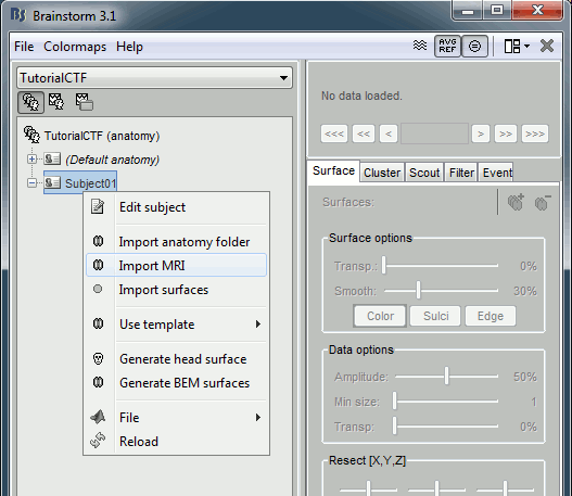
Select file "TutorialCtf/Anatomy/01.mri".
If you didn't download the CTF tutorial data yet, go back to the Tutorials page.The MRI viewer is displayed, together with a message box that tells you what to do. Follow the instructions. The MRI is already well oriented so you can directly process with the fiducials selection. You will see that three fiducials were already identified in the MRI file (NAS, LPA, RPA); you just need to add the three other ones (AC, PC, IH).
For instructions to find the fiducials, follow this link: CoordinateSystems.
Import surfaces
The MRI is available in the anatomy folder for Subject01. Let's now proceed with the surfaces. The envelopes we are going to import in this tutorial were extracted using BrainVISA, and their names and types may differ from other software solutions. To learn how to get those surfaces by yourself: read the tutorial for BrainVISA.
Right click on the subject node again, and click on "Import surfaces...". Select at the same time (holding Shift or Ctrl key) all the files in the directory "TutorialCtf/Anatomy/BrainVISA" (head, Lhemi, Rhemi). Click on "Open".
You should see the three surfaces in the database tree.
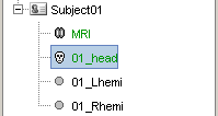
One has been identified automatically as a scalp (=head) surface, because its original filename contained the "scalp" keyword. Usually, Brainstorm identifies file types with this kind of tags in the file names.
The two other files were not identified automatically. They contain the envelopes of the left and right hemispheres of the brain, but Lhemi and Rhemi are not keywords that are identified automatically by Brainstorm.
Try to display the surfaces by double-clicking on them, or with the popup menu Display.
Downsample and merge surfaces
In the Surfaces tab, you can see the numbers of faces and vertices for each surface, and also display their faces (wireframe) with the Edges button. They look great, but their resolution is too high for the algorithms we will apply on them later, they need to be downsampled.
- Downsample:
Right-click on the head surface > Less vertices...: enter 7000, and press Ok.
Right-click on the Lhemi surface > Less vertices...: enter 7500, and press Ok.
Right-click on the Rhemi surface > Less vertices...: enter 7500, and press Ok.
- Three new surfaces appeared in the list, with the number of vertices as a suffix.
Group left and right hemisphere to build a Cortex surface:
Select Lhemi_7500V and Rhemi_7500V files at once (hold Ctrl key and left-click on both)
Right-click > Merge surfaces
A file called New surface appeared at the end of the list, rename it in Cortex (F2 key, or click twice on it but waiting between the two clicks, or right-click > Rename). Its icon should change automatically: the surface has been classified automatically as a Cortex (keyword that was recognized).
If you prefer calling it in an other way, you would have to specify manually that it is a cortex envelope: right-click > Set surface type > Cortex
Double-click on it to display it (or right-click > Display), and check in the Surfaces tab that the number of vertices is about 15000.
- Multiple surfaces of the same type:
Here you are in configuration where you have two surfaces that are classified as head.
- The one which is displayed in green is considered as the default one. It would be used automatically by all the functions that would need the head surface for this subject.
- Double-click on the other head surface to select it, it should turn green.
However, this is not the recommanded way to proceed, it might be confusing. To make things clear: always set as "Other" the surfaces you are not going to use in the source estimation process.
- A bit of cleaning:
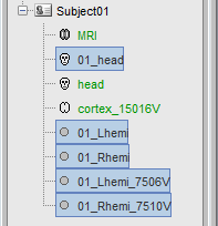
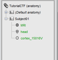
Rename the 01_head_SCS_7000V in Head.
Delete all the surfaces but the Head and Cortex (Delete key, or right-click>Delete).
Before:
 After:
Bug warning
Description: On some operating systems, it may happen that the tree is not refreshed well. Just after adding new files, the database tree can be displayed incompletely or can event appear completely empty. This bug occurs sometimes because the interactions between Matlab and Java are not always well synchronized.
Workaround: If this happens, just refresh the tree display with by either pressing the F5 key, or by changing the display mode. We'll try to fix this bug some day.
Check registration with MRI
Your Subject01 anatomy is ready for source estimation. But before going further, you should always check that surfaces and MRI are well registered. When performing those steps a bit too fast, it is really easy to end up with a cortex envelope that is not aligned with the MRI. None of the following steps in source estimation will check that for you, and the sources estimated would be completely wrong.
Right-click on the Cortex surface > MRI Registration > Check MRI/surface registration...
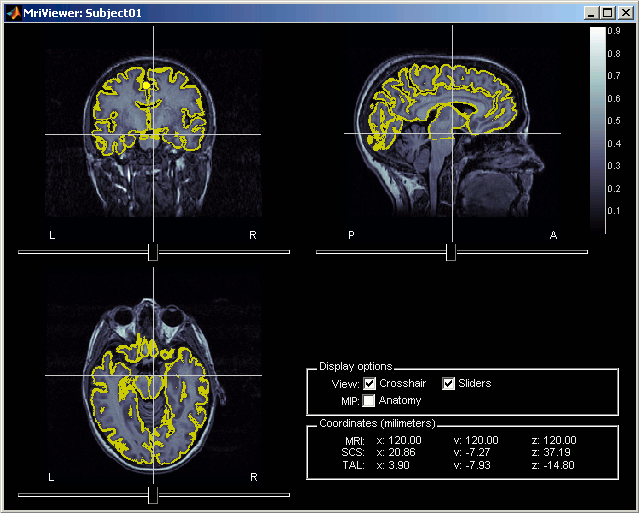
- The yellow lines represent the re-interpolation of the surface in the MRI volume. The computation may take a while, but the result will be stored in the surface file, and will be useful for other operations anyway.
Fix registration with MRI
In some rare cases, the surfaces may not be registered correctly with the MRI.
- If this happens, delete your MRI and surfaces and start again from scratch, it may be a manipulation mistake.
- If the result is not better and you don't know what happens, it is likely that the coordinate system used in your surface file is not handled by Brainstorm. There are still two emergency possibilities: pointing the fiducials on the head surface, and editing manually the surfaces. Both options give really unprecise results, but might help if nothing else is possible...
- You would not need to use this with this tutorial data, as the surfaces are already well registered with the MRI. But go through the following steps anyway, so that you know what to do in case this happens.
Defining the fiducials on head surface
- Of course it is possible only if you have the head surface.
Right-click on Cortex > MRI Registration > Align all surfaces (with MRI fiducials)...
You will be asked to point on the scalp surface the same fiducials as in the MRI (NAS, LPA, RPA). Click on a button in the toolbar (NAS, LPA or LPA), and point it on the surface. Repeat this operation for each fiducial.
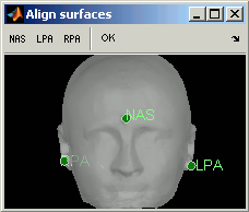
Do not click on OK. Normally you would click on OK button in toolbar, and it would realign all the subject's surfaces. However, here we don't want to alter our perfect subject, so just close the "Align surfaces" window, and the modifications will be ignored.
Manual alignment
- The goal is to realign graphically and interactively one surface on another.
Right-click on Cortex > MRI Registration > Align manually on... > Head
The orange surface is the one you are modifying, the grey one is the target. Move your mouse over the buttons in the toolbar to see what they do, select one you like, and then right-click + move up/downBR>>
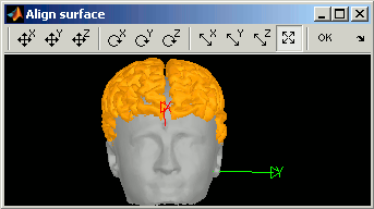
Do not click on OK. Close the window, and answer No to the question "Would you like to save the changes ?"
Check one last time that we didn't modify anything: Right-click on Cortex > Check alignment with MRI...
What happened on the hard drive
For most manipulations, it is not necessary to know exactly what is going on at the level of the real files, in Brainstorm database directory. But many things are not accessible from the Brainstorm interface, and you may find useful to manipulate some piece of data directly from the Matlab command window.
The right-click > File menu, accessible on all the nodes in Brainstorm database explorer, offers many tools to interact with the file system and the Matlab environment.
Where are the files ?
Several ways to reach a file:
Leave your mouse during a few seconds over any node in the database explorer, and a tooltip will appear, with the name and path of the corresponding file on hard drive.
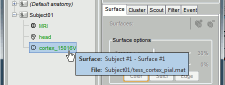
Paths are relative to current protocol path (brainstorm_database/TutorialCTF). What is displayed in Brainstorm window is a comment and may have nothing to do with the real file name. Eg. the Scalp surface's real file name is tess_cortex_concat.mat.
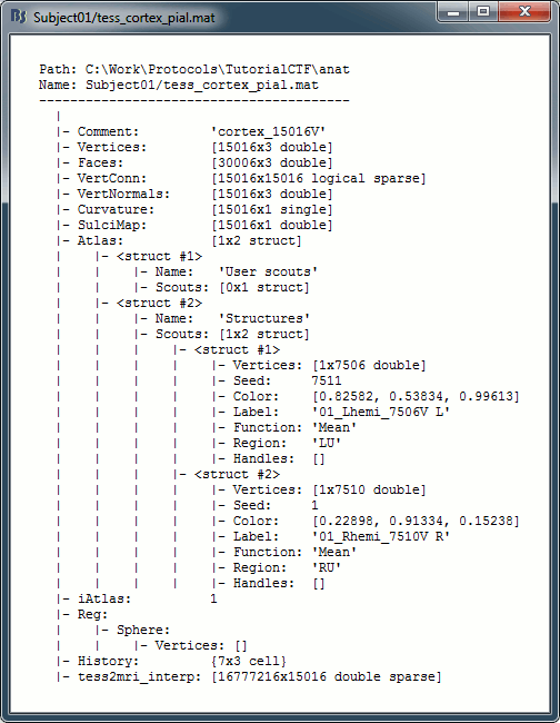
- Almost all the files in Brainstorm database (imported data or computation results) are in Matlab .mat format. As a consequence, you can load them really easily in the Matlab environment, where they appear as structures with several fields.
Popup menu: File
Right-click on any file: Many menus can lead you to the files and their contents, example with the Cortex node:
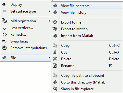
View file contents: Display all the fields in the corresponding Matlab .mat file, and the file absolute pat
View file history: Review the History field in the file, that records all the operations that were performed on the file since if was imported in Brainstorm

Export to file: Export in one of the supported mesh file format
Export to Matlab: Load the contents of the .mat file in the Matlab base workspace. It is then accessible from the Matlab command window:
Data exported as "surf"
>> surf
surf =
           Vertices: [3x15010 double]
              Faces: [29944x3 double]
            Comment: 'Cortex'
            History: {14x3 cell}
           VertConn: [15010x15010 logical]
        VertNormals: [3x15010 double]
          Curvature: [15010x1 single]
    tess2mri_interp: [16777216x15010 double]
>>
Import from Matlab: Replace the selected file with the content of a variable from the Matlab base workspace. Useful to save back in the database some structures that where exported and modified manually with the Matlab command window.
Go to this directory (Matlab): Change the current Matlab path, so that you can access the file from the Matlab Command window or the Matlab Current directory window
Show in file explorer: Open an explorer window in this directory (not working on all the systems...)
Open terminal in this folder: Start a system console in the file directory (Linux, Unix, MacOS only)
What are all those other files ?
If you look in your brainstorm_database/TutorialCTF directory, you'll find many other directories and files that are apparently not displayed in Braistorm database explorer.
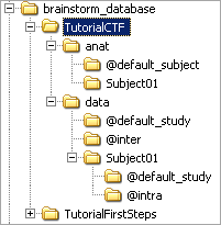
The protocol TutorialCTF is divided in Anatomy and Datasets directories:
Each subject in anat is described by an extra file: brainstormsubject.mat
Each condition in data is described by an extra a file: brainstormstudy.mat
anat/@default_subject: contains the files that are displayed in the (Default anatomy) node in database explorer
data/@default_study: used when files are shared between different subjects, node (Global common files)
data/@inter: results of inter-subject analysis
data/Subject01/@default_study: used when files are shared between different conditions in Subject01; node (Common files)
data/Subject01/@intra: results of intra-subject analysis (across different conditions)
Next
The anatomy of our subject is ready for source estimation, the next tutorial will explain ?how to import recordings.
