|
Size: 14145
Comment:
|
Size: 14423
Comment:
|
| Deletions are marked like this. | Additions are marked like this. |
| Line 1: | Line 1: |
| '''[WARNING: This page is part of the old tutorials, please refer to the [[Tutorials|new documentation]]]'''<<BR>><<BR>><<BR>> |
|
| Line 2: | Line 4: |
| ''Authors: Francois Tadel, John C Mosher, Richard Leahy, Sylvain Baillet'' |
|
| Line 15: | Line 19: |
| * The program is going to take the pre-stimulus values (= ''baseline'') for all the files that have been selected, which are supposed to be only noise, concatenate them, and then compute the covariance matrix for this big F matrix: <<BR>>!NoiseCov = (F - mean(F)) * (F - mean(F))' | * The program is going to take the pre-stimulus values (= ''baseline'') for all the files that have been selected, which are supposed to be only noise, concatenate them, and then compute the covariance matrix for this big F matrix: <<BR>>NoiseCov = (F - mean(F)) * (F - mean(F))' |
| Line 49: | Line 53: |
| * If you calculate the averages in Brainstorm, you don't have to worry about it, it is done automatically. It is only in the case you have imported in Brainstorm files that were averaged in another software, because the number of averaged trials was propably not saved in the file. | * If you calculate the averages in Brainstorm, you don't have to worry about it, it is done automatically. It is only in the case you have imported in Brainstorm files that were averaged in another software, because the number of averaged trials was probably not saved in the file. |
| Line 56: | Line 60: |
| Computationally speaking, this noise covariance matrix is very easy to calculate, the Brainstorm interface offers a lot of flexibilty to use the files and time windows you want to process. The real difficulty is to define what "noise" means. In your experiment, you want to use segments of recordings that contain only the noise of the sensors if possible, or segments of recordings that do not contain any of the brain signals of interest. This section is not directly useful for the current tutorial, but can be used as a reference for selecting the appropriate method in another experiment. | Computationally speaking, this noise covariance matrix is very easy to calculate, the Brainstorm interface offers a lot of flexibility to use the files and time windows you want to process. The real difficulty is to define what "noise" means. In your experiment, you want to use segments of recordings that contain only the noise of the sensors if possible, or segments of recordings that do not contain any of the brain signals of interest. This section is not directly useful for the current tutorial, but can be used as a reference for selecting the appropriate method in another experiment. |
| Line 59: | Line 63: |
| '''Empty room''': The MEG case is usually easier because we have access to real noise measurements, the MEG room just has to be empty. Record a few minutes right before bringing the subject in the MEG, or after the experiment is done. This would isolate only the noise from the sensors, which is what we are interested in in most cases.<<BR>>Additionnally, if you acquire several runs successively, or even several subjects, you can assume that the state of the sensors doesn't change much over the time. Therefore, you can re-use the same noise recordings and noise covariance matrix for several runs and subjects. | '''Empty room''': The MEG case is usually easier because we have access to real noise measurements, the MEG room just has to be empty. Record a few minutes right before bringing the subject in the MEG, or after the experiment is done. This would isolate only the noise from the sensors, which is what we are interested in most cases.<<BR>>Additionnally, if you acquire several runs successively, or even several subjects, you can assume that the state of the sensors doesn't change much over the time. Therefore, you can re-use the same noise recordings and noise covariance matrix for several runs and subjects. |
| Line 78: | Line 82: |
| == Feedback == <<EmbedContent(http://neuroimage.usc.edu/brainstorm3_register/get_feedback.php?Tutorials/TutNoiseCov)>> |
==== Forum posts ==== * EEG reference: http://neuroimage.usc.edu/forums/showthread.php?1525#post6718 |
| Line 83: | Line 87: |
<<EmbedContent(http://neuroimage.usc.edu/bst/get_feedback.php?Tutorials/TutNoiseCov)>> |
[WARNING: This page is part of the old tutorials, please refer to the new documentation]
Tutorial 7: Noise covariance matrix
Authors: Francois Tadel, John C Mosher, Richard Leahy, Sylvain Baillet
The source reconstruction process requires an estimation of the noise level in the recordings. Ideally, we want to represent only the noise of the sensors, but we can also use a baseline of resting recordings. The main problem is in fact to identify segment of recordings that we can consider as "noise", or at least that do not contain any of the brain activity of interest. This tutorial shows how to compute the noise covariance matrix from the pre-stimulation baseline of the two averaged files we have in the database.
Compute from recordings
Select protocol TutorialCTF, switch to the Functional data (sorted by subjects) view.
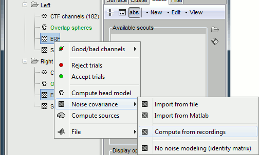
To estimate the noise covariance matrix, we need to use only the average of the MEG recordings, and not the standard deviations. Select the two ERF files at the same time (holding the Ctrl key, or Command on Macs), then right-click on one of them.

- The "Noise covariance" menu includes:
Import from file: Uses a matrix that was computed previously using the MNE software.
Import from Matlab: Import from any [nChannels, nChannels] matrix in Matlab workspace.
Compute from recordings: Use the selected recordings to estimate the noise covariance.
No noise modeling: Do not compute the noise covariance matrix from noise recordings. Instead, create a file that contains an identity matrix. In the inverse modeling, this is equivalent to the assumption that the noise in the recordings is homoskedastic,and equivalent for all the sensors.This is the menu to use when you really don't have access to any noise information, or when you don't have any option to identify this noise (for instance if you are studying ongoing activity with EEG).
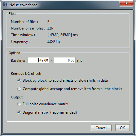
Select "Compute from recordings", the options window appears:

The program is going to take the pre-stimulus values (= baseline) for all the files that have been selected, which are supposed to be only noise, concatenate them, and then compute the covariance matrix for this big F matrix:
NoiseCov = (F - mean(F)) * (F - mean(F))'- The top part of this window shows a summary of the files that have been selected: 2 files at 1250Hz. Total: 126 time samples.
- In the bottom part, you can define some options:
Baseline: You can specify what you consider as the pre-stimulus time window in your recordings. By default it takes all the time instants before 0ms, but you might need to redefine this depending on your experiment.
Remove DC Offset: Define how to remove the average from each file: file by file, or globally.
Output: Compute either a full noise covariance, or just a diagonal matrix (only the variances of the channels). It's better to use a full noise covariance matrix, but only when you have a lot of time points to estimate it properly, which is not the case here. Just always keep the default selection unless you know exactly what you are doing, Brainstorm detects what the preferred option is for every case.
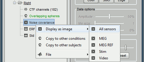
Click on OK. Observe that two new files appeared in the database, one for each condition. Each of them contains the same [nChannels x nChannels] noise covariance matrix. Right-click on one of them:

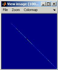
Display as image: Shows the noise covariance matrix as an indexed image. This can be useful to quickly check the quality of the recordings. The noisier channels are indicated by red points. You can display the noise covariance for all the sensors at once, or for each sensor type separately. Double-clicking on the file display all the sensors.

Copy to other conditions: Copy this noise covariance matrix to all the other conditions from the same subject.
Copy to other subjects: Copy this noise covariance matrix to all the conditions of all the subjects in the database.
You can also copy a noise covariance file to another condition/subject just like any other file: using the popup menus File > Copy/Paste, or the keyboard shortcuts Ctrl+C and Ctrl+V.
Note: The more time samples you have for the estimation of the noise covariance, the more accurate the source estimation. If you have many files available for the same subject / same run, always use all of them. Select all the files at the same time (or the subject, when you don't have different types of files like our "Std" files here), and start the computation for all of them at the same time. If you run the same process several times for the same subjects/conditions on different files, the noise covariance file is just overwritten at each time.
Noise covariance from another dataset
In order to get a good estimation of the noise, we need much more time samples than what we have in an averaged file. Also, the pre-stimulation baseline might not be a very good estimation of the noise of the sensors. You have several options available to get better results, by using different segments of recordings than the ones that you are analyzing.
The only constraint: you need to apply the exact same pre-processing operations to the recordings you use for the estimation of the noise covariance, and to the recordings for which you are reconstructing the sources: frequency filters, resampling, re-referencing...
Use single trials: If you have the single trials from which the average file was computed,
- Create another condition in your subject and import the single trials in it,
Estimate the noise covariance on these single trials only (right-click on the new condition node > Noise covariance > Compute...). Use only the pre-stimulus baseline.
Right-click on the new noise covariance file > Noise covariance > Apply to all conditions. This copies the noise covariance file in the conditions of your averaged files. Alternatively, use the Copy/Paste menus or shortcuts.
Use a real baseline: If you have recorded some resting periods during the experiment, or some empty room measurements, you can use them exactly as in the previous case.
- Import the blocks of raw recordings in the database in a new condition
- Compute the noise covariance using the entire time window (it is supposed to be noise everywhere)
- Copy to other conditions
Use the original continuous file: Same thing as previously, but skipping the import part. You can compute directly the noise covariance from a RAW file:
Right-click on your subject node > Review RAW file. (the management of continuous files in native format is detailed in an advanced tutorial: ?Review raw recordings and edit markers)
Right-click on Link to raw file > Noise covariance > Compute from recordings. Then select the time window to use as a baseline (subject resting or empty room).
- Copy to other conditions.
Import from another software: If you have pre-processed your recordings with the MNE software, you might already have a nice noise covariance matrix available in a -cov.fif file. Just import it in the average conditions (right-click on condition > Noise covariance > Import from file)
Note for averaged files: If you import or compute a noise covariance matrix based on a set of RAW recordings (not averaged), and then use it to estimate sources for averaged recordings, you may have to set manually the number of trials that were used to compute the average.
- If you calculate the averages in Brainstorm, you don't have to worry about it, it is done automatically. It is only in the case you have imported in Brainstorm files that were averaged in another software, because the number of averaged trials was probably not saved in the file.
To check if this information is stored in the database: right click on the averaged file for which you want to estimate the sources. Menu File > View file contents. If you see "nAvg = 1", the noise covariance matrix will not be used correctly on that file. To fix this problem:
Right-click on the averaged file > File > Export to Matlab > "data"
- In the Matlab command window, type: "data.nAvg = nTrials;" (replace nTrials with the actual number of trials from which the average was computed)
Right-click on the averaged file > File > Import from Matlab > "data"
Discussion
Computationally speaking, this noise covariance matrix is very easy to calculate, the Brainstorm interface offers a lot of flexibility to use the files and time windows you want to process. The real difficulty is to define what "noise" means. In your experiment, you want to use segments of recordings that contain only the noise of the sensors if possible, or segments of recordings that do not contain any of the brain signals of interest. This section is not directly useful for the current tutorial, but can be used as a reference for selecting the appropriate method in another experiment.
MEG
Empty room: The MEG case is usually easier because we have access to real noise measurements, the MEG room just has to be empty. Record a few minutes right before bringing the subject in the MEG, or after the experiment is done. This would isolate only the noise from the sensors, which is what we are interested in most cases.
Additionnally, if you acquire several runs successively, or even several subjects, you can assume that the state of the sensors doesn't change much over the time. Therefore, you can re-use the same noise recordings and noise covariance matrix for several runs and subjects.
Resting baseline: Alternatively, when studying evoked responses (aka event-related responses), you can use a few minutes of recordings where the subject is resting, ie. not performing the task. Record those resting segments before or after the experiment, or before/after each run. This approach considers the resting brain activity as "noise", and the sources estimated for the evoked response are going to be preferentially the ones that were not activated during the resting period.
Pre-stimulation baseline: It can also be a valid approach to use the pre-stimulation baseline of the individual trials to estimate the noise covariance. But keep in mind that in this case, everything in your pre-stimulation baseline is going to be attenuated in the source reconstruction, noise and brain activity. Therefore, your stimuli have to be distant enough in time so that the response to a stimulus is not recorded in the "baseline" of the following one. For repetitive stimuli, randomized delays between stimuli can help avoiding expectation effects in the baseline.
EEG
The EEG case is typically more complicated. It is not possible to estimate the noise of the sensors only. Only the two other approaches described for the MEG are still valid:
resting baseline and pre-stimulation baseline.
The noise level of the electrodes recordings depends primarily on the quality of the connection with the skin, which varies a lot from a subject to another, or even during the acquisition of one single subject. The conductive gel or solution used on the electrodes tends to dry, and the electrode cap can move. Therefore, it is very important to use one channel file per subject, hence one noise covariance per subject. In some specific cases, if the quality of the recordings varies a lot over the time, it can be interesting to split long recordings in different runs, with different noise covariance matrices too.
EEG and resting state
When studying the resting brain, you cannot use resting recordings as a noise baseline. For MEG the best choice is to use empty room measurements. For EEG, you can chose between two different approaches: using the sensors variance, or not using any noise information.
Option #1: Calculate the covariance over a long segment of the resting recordings, but save only the diagonal, ie. the variance of the sensors. To do so from the interface: just check the box "Diagonal matrix" in the options window.
Option #2: Select "No noise modeling" in the popup menu. This would use an identity matrix instead of a noise covariance matrix (equal, unit variance of noise on every sensor). The problem with this approach is that an electrode with a higher level of noise is going to be interpreted as a lot of activity in its region of the brain.
Noise and epilepsy
Analyzing a single interictal spike, using either EEG and MEG data, we are faced with a similar problem in defining what is noise. The brain activity before and after the spike can even be very informative about the spike's generation, particularly if it is part of a sequence of interictal activity that precedes ictal (seizure) onset. Defining a segment of time adjacent the spike as "background" may not be practical. In practice, however, we often can find a temporal region of spontaneous brain activity in the recordings that appears adequate for declaring as background, even in the epileptic patient. As discussed above, MEG has the additional option of using empty room data as a baseline, an option not available in EEG.
We thus have the same options as above:
Option #1a: Compute the noise covariance statistics from blocks of recordings away from the peak of any identified interictal spike, and keep only the diagonal (the variance of the sensors).
Option #1b: If a large period of time is available, calculate the full noise covariance.
Option #2(MEG): Use empty room data as the baseline.
Option #3: Select "No noise modeling" in the popup menu (identity matrix, unit variance of noise on every sensor).
Forum posts
Next
Next tutorial: ?source estimation.
