|
Size: 18538
Comment:
|
Size: 18531
Comment:
|
| Deletions are marked like this. | Additions are marked like this. |
| Line 4: | Line 4: |
| This tutorial fills the gap between the previous tutorial (review and clean continuous recordings), and the introduction tutorials (source analysis of evoked responses). It explains how to epoch the recordings, do some more pre-processing on the single trials, and then calculate their average. For this tutorial, we are going to use the protocol '''!TutorialRaw''' created in the two previous tutorials: [[Tutorials/TutRawViewer|Review continuous recordings and edit markers]] and [[Tutorials/TutRawSsp|Artifact cleaning]]. If you have not followed these tutorials yet, please do it now. | This tutorial fills the gap between the previous tutorial (review and clean continuous recordings), and the introduction tutorials (source analysis of evoked responses). It explains how to epoch the recordings, do some more pre-processing on the single trials, and then calculate their average. For this tutorial, we are going to use the protocol '''TutorialRaw''' created in the two previous tutorials: [[Tutorials/TutRawViewer|Review continuous recordings and edit markers]] and [[Tutorials/TutRawSsp|Artifact cleaning]]. If you have not followed these tutorials yet, please do it now. |
| Line 41: | Line 41: |
| Double-click on the first trial for the "left" condition. Then right-click on the figure > '''Next data file''', or use the keyboard shortcut '''F3 '''to jump to the next trial. This way you can quickly review all the trials, to make sure that there is no obvious problem in the recordings. If you haven't reviewed manually all the recordings in the continuous mode, and marked all the bad segments, it is a good time to do it now. | Double-click on the first trial for the "left" condition. Then right-click on the figure > Navigator > '''Next data file''', or use the keyboard shortcut '''F3 '''to jump to the next trial. This way you can quickly review all the trials, to make sure that there is no obvious problem in the recordings. If you haven't reviewed manually all the recordings in the continuous mode, and marked all the bad segments, it is a good time to do it now. |
| Line 101: | Line 101: |
| Close all the figures, clear the Process1 list (right-click > clear, or select+delete key), and drag and drop all the trials and all the averages (or simply the two left and right condition folders). Select the process "'''Pre-process > Add time offset'''". Set the time offset to '''-4.2 ms''', to bring back this stimulation peak at 0ms. Select also the "'''Overwrite initial files'''" option, to avoid too many duplications of unnecessary files in the database. | Close all the figures, clear the Process1 list (right-click > clear, or select+delete key), and drag and drop all the trials and all the averages (or simply the two left and right condition folders). Select the process "'''Pre-process > Add time offset'''". Set the time offset to '''-4.2 ms''', to bring back this stimulation peak at 0ms. Select also the "'''Overwrite input files'''" option, to avoid too many duplications of unnecessary files in the database. |
| Line 177: | Line 177: |
| == Feedback == |
C3. Epoching and averaging
Authors: Francois Tadel, Elizabeth Bock, John C Mosher, Sylvain Baillet
This tutorial fills the gap between the previous tutorial (review and clean continuous recordings), and the introduction tutorials (source analysis of evoked responses). It explains how to epoch the recordings, do some more pre-processing on the single trials, and then calculate their average. For this tutorial, we are going to use the protocol TutorialRaw created in the two previous tutorials: ?Review continuous recordings and edit markers and ?Artifact cleaning. If you have not followed these tutorials yet, please do it now.
Contents
Import in database
The raw file viewer provides a rapid access to the recordings, but most of operations cannot be performed directly on the continuous files: most of the pre-processing functions, averaging, time-frequency analysis and statistical tests can only be applied on blocks of data that are saved in the database (ie. "imported"). After reviewing the recordings and editing the event markers, you have to "import" the recordings in the database to go with further analysis.
Right-click on the file with power line correction: Raw | notch(60Hz 120Hz 180Hz) > Import in dabase

Warning: If you right-click on the subject node > Import EEG/MEG, and select the tutorial .ds dataset, you would be able to import blocks of the continuous file in the database, but you would not have access to the modified events list or the SSP operators. Therefore, you would not import data cleaned of ocular and cardiac artifacts. The modified events list and the signal space projectors are saved only in the "Link to raw file" in the Brainstorm database, not in the initial continuous file.
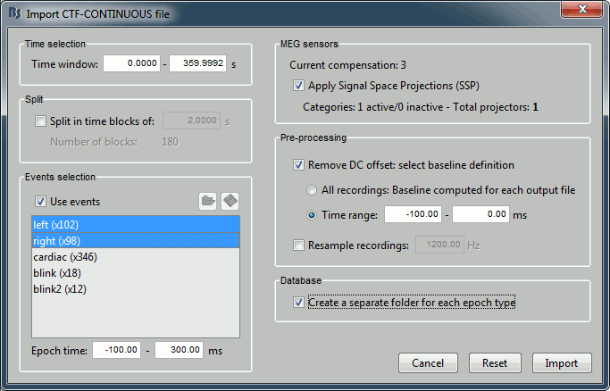
Set the import options as they are represented in this figure:
Time window: Time range of interest. We are interested by all the stimulations, so do not change this parameter; the default values always represent the entire file.
Split: Useful to import continuous recordings without events, to import successive chunks of the same duration. We do not need this here.
Events selection: Check the "Use events" option, and select both "left" and "right". The number in the parenthesis represents the number of occurrences of this event in the selected time window (would change if you modify the time definition on top of the figure)
Epoch time: Time segment that is extracted around each marker and saved in the database. Set it to [-100, +300] ms
Use Signal Space Projections: Use the active SSP projectors calculated during the previous pre-processing steps. Keep this option selected.
Remove DC Offset: Check this option, and select: Time range: [-100, 0] ms. For each epoch, this will: compute the average of each channel over the baseline (pre-stimulus interval: -100ms to 0ms), and subtract it from the channel at every time instants (full epoch interval: [-100,+300]ms).
This option removes the baseline value of each sensor, ie. the continuous (DC) offset that is added permanently on top of the recordings of interest. In MEG, the sensors record variations around a somewhat arbitrary level, therefore this operation is always needed, unless it was already applied during one of the pre-processing steps.
Note that a high-pass filter with a very low frequency (for instance 0.3Hz) can replace efficiently this DC correction. If a high-pass filter has already been applied to the recordings, you may want to unselect this option.Resample recordings: Keep this unchecked
Create a separate folder for each epoch type: If selected, a new folder is created for each event type (here, it will create two folders in the database: "left" and "right"). If not selected, all the epochs are saved in a new folder, the same one for all the events, that has the same name as the initial raw file.
Click on Import and wait. At the end, you are asked whether you want to ignore one epoch that is shorter than the others. This happens because the acquisition of the MEG signals was stopped less than 300ms after the last stimulus trigger was sent. Therefore, the last epoch cannot have the full [-100,300]ms time definition. This shorter epoch would prevent us from averaging all the trials easily. As we already have enough repetitions in this experiment, we can just ignore it. Answer Yes to this question to discard the last epoch.

Two new conditions containing two groups of trials appeared in the database. To expand a group of trials and get access to the individual epochs: double-click on it or click on the "+" next to it.
The SSP projectors calculated in the previous tutorial were applied on the fly when reading from the continuous file. Those epochs are clean from eye blinks and power line contamination.
All the files available in the (Common files) folder are also shared for those new folders "left" and "right".
Review the individual trials
Double-click on the first trial for the "left" condition. Then right-click on the figure > Navigator > Next data file, or use the keyboard shortcut F3 to jump to the next trial. This way you can quickly review all the trials, to make sure that there is no obvious problem in the recordings. If you haven't reviewed manually all the recordings in the continuous mode, and marked all the bad segments, it is a good time to do it now.
To mark a trial as bad manually, you have three methods:
Right-click on the trial file in the database > Reject trial
Right-click on the figure > Reject trial
Use the keyboard shortcut Control+B
To set all the trials back as good in a group: right-click on the trials group or the condition > Accept bad trials.
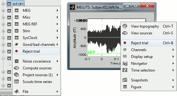
When a trial is tagged as bad, its icon in the database explorer shows a red mark.

All the bad trials are going to be ignored in the rest of the analysis, because they are ignored by the Process1 and Process2 tabs. If you drag and drop the 101 left trials in the Process1 list, with one trial marked as bad, the summary of the selected files on top of the tab would show only 100 data files.

To learn how to mark only individual channels as bad instead of the entire trial, please go back to the introduction tutorial ?Exploring the recordings.
The process "Artifacts > Detect bad channels: peak-to-peak" can help you detect automatically some bad trials based on a peak-to-peak amplitude threshold. Drag and drop all the trials from the left condition in the Process1 list, and select this process. For each trial, it detects the channels that have a peak-to-peak amplitude (maximum value - minimum value) that is above a rejection threshold (too noisy) or below a rejection threshold (no signal). You can define different thresholds for different channel types. The options are:
Time window: Time range on which the peak-to-peak amplitude is calculated on each trial
Thresholds: Rejection and detection thresholds for each sensor type.
For CTF recordings, use the "MEG gradio" category, and ignore the "/cm (x 0.04)" indication, that is valid only for Neuromag systems. Set the MEG gradio thresholds to [0, 2000] fT, to detect the MEG channels that have a peak-to-peak amplitude superior to 2000fT.Reject only the bad channels: This would tag as bad only the detected channels, but would not tag the trial itself as bad.
Reject the entire trial: This would tag as bad the trial if there is at least one channel file identified as bad.
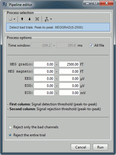
For this current dataset, the quality of the recordings is remarkably good, we don't need to mark any trial as bad. So right-click on the group of "left" trials > Accept trials, to set them all as good.
Averaging
Drag and drop the two lists of trials (or the two condition folders) in the Process1 list, and run the process "Average > Average files", with the option "Average by condition (subject average)". This will group the trials by conditions, and calculate one average per condition and subject. The option "By condition (grand average)" would average each condition for all the subjects together, but as there is only one subject in this case, the result would be same. The other options would generate one average file per subject ("by subject"), one average file per group of trials and per subject ("by trial group"), or only one average no matter what the input is ("everything").
The function to apply is the regular arithmetic average. The option "Keep all the events from the individual epochs" would group all the event markers present in all the epochs and save them in the new averaged file. It can be useful to check the relative position of the artifacts or the subject responses, or quickly detect some unwanted configuration such as a subject who would constantly blink right after a visual stimulus. We don't really need this here, leave this option unselected.
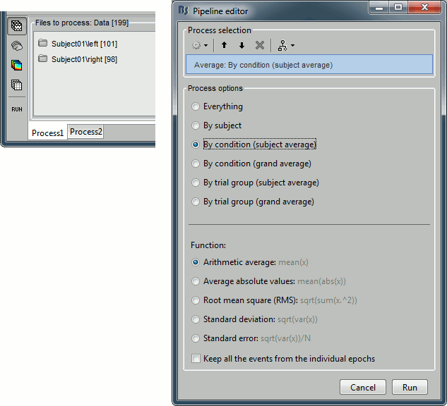
It creates two files: "Avg: left" and "Avg: right".
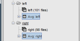
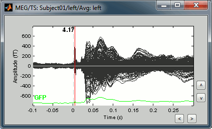
Double-click on the "Avg: Left" file to display the MEG recordings for this file (or right-click > MEG > display time series). It shows a very typical an clean evoked response, with a very high signal-to-noise ratio.
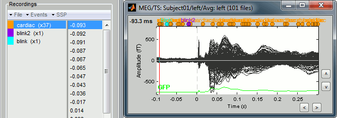
Just for the records, this is how it would look like if we had selected the option "Keep all the events from the individual epochs". The summary of the markers of all the epochs is: 37 heartbeats and 2 blinks.
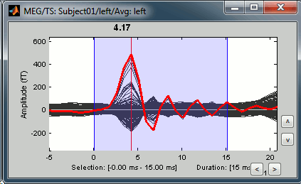
Stimulation artifact
Now zoom around 4ms in time (mouse wheel, or two figures up/down on macbooks) and amplitude (control + zoom). Notice this very strong and sharp peak followed by fast oscillations. This is an artifact due to the electric stimulation device. In the stimulation setup: the stimulus trigger is initiated by the stimulation computer and sent to the electric stimulator. This stimulator generates an electric pulse that is sent to electrodes on the subject's wrists. This electric current flows in the wires and the in the body, so it also generates a small magnetic field that is captured by the MEG sensors. This is what we observe here at 4ms.
This means that whenever we decide to send an electric stimulus, there is a 4ms delay before the stimulus is actually received by the subject, due to all the electronics in between. Which means that everything is shifted by 4ms in the recordings. Those hardware delays are unavoidable and should be quantified precisely before starting scanning subjects or patients.
Then you have two options: either you remember it and subtract the delays when you publish your results (there is a risk of forgetting about them), or you fix the files right now by fixing the time reference in all the files (there is a risk of forgetting to fix all the subjects/runs in the same way). Let's illustrate this second method now.
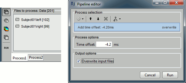
Close all the figures, clear the Process1 list (right-click > clear, or select+delete key), and drag and drop all the trials and all the averages (or simply the two left and right condition folders). Select the process "Pre-process > Add time offset". Set the time offset to -4.2 ms, to bring back this stimulation peak at 0ms. Select also the "Overwrite input files" option, to avoid too many duplications of unnecessary files in the database.
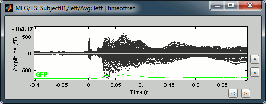
This fixes the individual trials and the averages. Double-click on the "Avg: left" file again to observe that the stimulation artifact is now occurring at 0ms exactly, which means that t=0s represents the time when the electric pulse is received by the subject.
Online filter
As introduced in the previous tutorials, you can add an online visualization filter to make the traces and the topographies look smoother. We suggest in this case a low-pass filter at 120Hz, because it shows very smooth traces, but all the waves we are interested in are still clearly visible in the MEG time series figure.

Explore the average
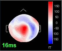
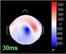
Open the time series for the "Avg: left". Then press Control+T, to see on the side a spatial topography at the current time point. Then observe what is happening between 0ms and 100ms. Start at 0ms and play it like a movie using the arrow keys left and right, to follow the brain activity millisecond by millisecond:
16 ms: First response, the sensory information reaches the right somatosensory cortex (S1)
30 ms: Stronger and more focal activity in the same region, but with a source oriented in the opposite direction (S1)
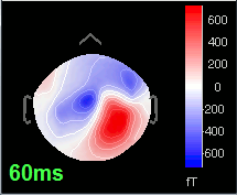
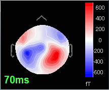
60 ms: Activity appearing progressively in a more lateral region (S1 + S2)
70 ms: Activity in the same area in the left hemisphere (S2 left + S2 right)
Source analysis
Let's reproduce the same observations at the source level. The concepts related with the source estimation are not discussed here; for more information, refer to the introduction tutorials #6 to #8.
First, delete all the files related with the source estimation calculated in the previous tutorials, available in the (Common files) folder: the head model, the noise covariance and inverse model. We can now provide a better estimate of the noise (affects the inverse model), and we defined new SSP operators (affects the head model).
Head model
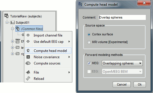
Right-click on any node that contains the channel file (including the channel file itself), and select: "Compute head model". Leave all the default options: cortex source space, and overlapping spheres. The lead field matrix is saved in file "Overlapping spheres" in (Common files).
Noise covariance matrix
To estimate the sources properly, we need an estimation of the noise level for each sensor. A good way to do this is to compute the covariance matrix of the concatenation of the baselines from all the trials in both conditions.
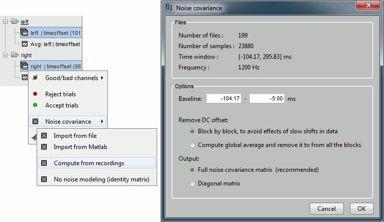
- Select at the same time the two groups of trials (right and left). To do this: hold the Control (or Cmd on Macs) key and click successively on the Right and the Left trial lists.
Right-click on one of them and select: Noise covariance > Compute from recordings. Set the baseline to [-104,-5] ms, to consider as noise everything that happens before the beginning of the stimulation artifact. Leave the other options to the default values. Click on Ok.
This operation computes the noise covariance matrix based on the baseline of all the good trials (199 files). The result is stored in a new file "Noise covariance" in the (Common files) folder.
Inverse model
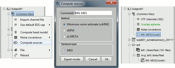
Right-click on (Common files), on the head model or on the subject node, and select "Compute sources". A shared inversion kernel is created in (Common files); a link node is now visible for each recordings file, single trials and averages. For more information about what those links mean and the operations performed to display them, please refer to the tutorial #8 "Source estimation".
Explore the sources
Right-click on the sources for the left average > Cortical activations > Display on cortex, or simply double click on the file. Go to the main response peak at t = 30ms, and increase the amplitude threshold to 100%. You see a strong activity around the right primary somatosensory cortex, but there are still lots of brain areas that are shown in plain red (value >= 100% maximum of the colorbar ~= 280 pA.m).
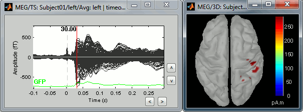
The colorbar maximum is set to an estimation of the maximum source amplitude over the time. This estimation is done by finding the time instant with the highest global field power on the sensors (green trace GFP), estimating the sources for this time only, and then taking the maximum source value at this time point. It is a very fast estimate, but not very reliable; we use it because calculating the full source matrix (all the time points x all the sources) just for finding the maximum value would be too long.
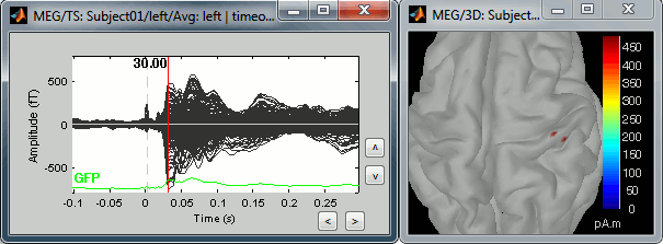
In this case, the real maximum is probably higher than what is used by default. To redefine the colorbar maximum: right-click on the 3D figure > Colormap: sources > Set colorbar max value. Set the maximum to 480 pA.m, or any other value that would lead to see just one very focal point on the brain at 30ms.
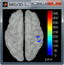
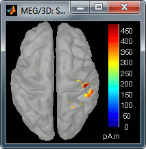
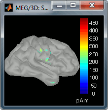
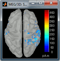
Go back to the first small peak at t=16ms, and lower the threshold to 10%. Then do what you did with at the sensor level: follow the information processing in the brain until 100ms, millisecond by millisecond, adapting the threshold and the camera position when needed:
16 ms (top-left): First response, primary somatosensory cortex (S1 right)
30 ms (top-right): S1 right
60 ms (bottom-left): Secondary somatosensory cortex (S2 right)
70 ms (bottom-right): Activity ipsilateral to the stimulus (S2 left + S2 right)
Scripting
All the operations that have been introduced in the last three tutorials can be reproduced easily from a Matlab script. This is illustrated in the tutorial Full analysis with one script.
This script is available in the Brainstorm distribution: brainstorm3/toolbox/script/tutorial_raw.m
