|
Size: 4649
Comment:
|
Size: 7096
Comment:
|
| Deletions are marked like this. | Additions are marked like this. |
| Line 9: | Line 9: |
| * In the Event tab: select the menu Import > Import > Import in database (only when the file viewer is open), * In the database tree: Right-click on the nodes "Link to raw file" > Import in database. Now, right-click on the file with power line correction:''' Raw | sin(60Hz 120Hz 180Hz) > Import in dabase''' |
Right-click on the file with power line correction:''' Raw | sin(60Hz 120Hz 180Hz) > Import in dabase''' |
| Line 16: | Line 13: |
| You would get the same menu from the event tab, when the file viewer is open: menu Import > Import in database. __Warning__: If you right-click on the subject node > Import EEG/MEG, and select the tutorial .ds dataset, you would be able to import blocks of the continuous file in the database, but you would not have access to the modified events list or the SSP operators. Therefore, you would not import data cleaned for the ocular and cardiac artifacts. The modified events list and the signal space projectors are saved only in the "Link to raw file" in the Brainstorm database, not in the initial continuous file. |
__Warning__: If you right-click on the subject node > Import EEG/MEG, and select the tutorial .ds dataset, you would be able to import blocks of the continuous file in the database, but you would not have access to the modified events list or the SSP operators. Therefore, you would not import data cleaned of ocular and cardiac artifacts. The modified events list and the signal space projectors are saved only in the "Link to raw file" in the Brainstorm database, not in the initial continuous file. |
| Line 24: | Line 19: |
| * '''Time window''': Time range of interest. Now we want to keep the whole time definition, we are interested by all the stimulations, so leave the default values | * '''Time window''': Time range of interest. We are interested by all the stimulations, so do not change this parameter; the default values always represent the entire file. |
| Line 26: | Line 21: |
| * '''Events selection''': Check the "Use events" option, and select both "left" and "right". The value between parenthesis represents the number of occurrences of this event in the selected time window (would change if you modify the time definition on top of the figure) * '''Epoch time''': Time segment that is extracted around each marker, to create the epochs that are saved in the database. Set it to [-100, +300] ms |
* '''Events selection''': Check the "Use events" option, and select both "left" and "right". The number in the parenthesis represents the number of occurrences of this event in the selected time window (would change if you modify the time definition on top of the figure) * '''Epoch time''': Time segment that is extracted around each marker and saved in the database. Set it to [-100, +300] ms |
| Line 29: | Line 24: |
| * '''Remove DC Offset''': Check this option, and select: Time range: [-100, 0] ms. For each epoch, this will: compute the average of each channel over the baseline (pre-stimulus interval: -100ms to 0ms), and subtract it from the channel at all the times in [-100,+300]ms. | * '''Remove DC Offset''': Check this option, and select: Time range: [-100, 0] ms. For each epoch, this will: compute the average of each channel over the baseline (pre-stimulus interval: -100ms to 0ms), and subtract it from the channel at every time instants (full epoch interval: [-100,+300]ms). |
| Line 33: | Line 28: |
| Click on Import and wait. In the end, you are asked whether you want to ignore one epoch that is shorter than the others. This happens because the acquisition of the MEG signals was stopped less than 300ms after the last stimulus trigger was sent. Therefore, the last epoch cannot have the full [-100,300]ms time definition. This shorter epoch would prevent us from averaging all the epochs easily. As we already have enough repetitions in this experiment, we can ignore it. Answer '''Yes''' to this question to discard the last epoch. | Click on Import and wait. At the end, you are asked whether you want to ignore one epoch that is shorter than the others. This happens because the acquisition of the MEG signals was stopped less than 300ms after the last stimulus trigger was sent. Therefore, the last epoch cannot have the full [-100,300]ms time definition. This shorter epoch would prevent us from averaging all the trials easily. As we already have enough repetitions in this experiment, we can just ignore it. Answer '''Yes''' to this question to discard the last epoch. |
| Line 37: | Line 32: |
| Two new conditions containing two groups of trials appeared in the database. The groups of trials are not expanded by default, to have the database tree displayed faster. To expand a list and get access to the individual trials: double click on it, or right-click on the list > Expand. | Two new conditions containing two groups of trials appeared in the database. The groups of trials are not expanded by default, in order to have the database tree displayed faster. To expand a list and get access to the individual trials: double click on it, or right-click > Expand. |
| Line 39: | Line 34: |
| The SSP projectors were applied on the fly when reading from the continuous file. Those epochs are clean from everything that we corrected in the previous tutorial: the eye blinks and the power line contamination. | The SSP projectors calculated in the previous tutorial were applied on the fly when reading from the continuous file. Those epochs are clean from eye blinks and power line contamination. All the files available in the ''(Common files)'' folder are also shared for those new folders "left" and "right". |
| Line 42: | Line 39: |
== Review the individual trials == Double-click on the first trial for the "left" condition. Then right-click on the figure > '''Next data file''', or use the keyboard shortcut '''F3 '''to jump to the next trial. This way you can quickly review all the trials, to make sure that there is no obvious problem in the recordings. If you haven't reviewed manually all the recordings in the continuous mode, and marked all the bad segments, it is a good time to do it now. To mark a trial as bad manually, you have three methods: * Right-click on the trial file in the dabase > '''Reject trial''' * Right-click on the figure > '''Reject trial''' * Use the keyboard shortcut '''Control+B''' * To set all the trials back as good in a group: right-click on the trials group or the condition > Accept bad trials. {{attachment:rejectManual.gif|importDb.gif}} When a trial is tagged as bad, its icon in the database explorer show a red mark. {{attachment:rejectTree.gif|importDb.gif}} All the bad trials are going to be ignored in the rest of the analysis, because they are ignored by the Process1 and Process2 tabs. If you drag and drop the 101 left trials in the Process1 list, with one trial marked as bad, the summary of the selected files on top of the tab would show only 100 data files. {{attachment:rejectProcess.gif|importDb.gif}} One process can help you detect automatically some bad trials based on a peak-to-peak value threshold. Drag and drop all the trials from the '''left''' condition in the Process1 list, and select the process "'''Artifacts > Detect bad channels: peak-to-peak'''". For each trial, it detects the channels that have a peak-to-peak amplitude (maximum value - minimum value) that is over a rejection threshold (too noisy) or below a rejection threshold (no signal). You can define different thresholds for different channel types. The options are: * '''Time window''': Time range for which the peak-to-peak value is calculated on each trial * '''Thresholds''': Rejection and detection thresholds for each sensor type. For CTF recordings, use the "MEG gradio" category, and ignore the "/cm (x 0.04)" indication, that is valid only for Neuromag systems. Set the '''MEG gradio''' thresholds to '''[0, 2000] fT''', to consider as bad any MEG channel that would have a peak-to-peak amplitude superior to 2000fT. * '''Reject only the bad channels''': This would tag as bad only the detected channels, but would not tag the trial as bad. * '''Reject the entire trial''': This would tag as bad the trial if there is at least one channel file identified as bad. {{attachment:rejectOptions.gif|importDb.gif}} |
Epoching and averaging
This tutorial fills the gap between the previous tutorial (review and clean continuous recordings), and the introduction tutorials (source analysis of evoked responses). It explains how to epoch the recordings, do some more pre-processing on the single trials, and then calculate their average.
Import in database
The raw file viewer provides a rapid access to the recordings, but most of operations cannot be performed directly on the continuous files: most of the pre-processing functions, averaging, time-frequency analysis and statistical tests can only be applied on blocks of data that are saved in the database (ie. "imported"). After reviewing the recordings and editing the event markers, you have to "import" the recordings in the database to go with further analysis.
Right-click on the file with power line correction: Raw | sin(60Hz 120Hz 180Hz) > Import in dabase

Warning: If you right-click on the subject node > Import EEG/MEG, and select the tutorial .ds dataset, you would be able to import blocks of the continuous file in the database, but you would not have access to the modified events list or the SSP operators. Therefore, you would not import data cleaned of ocular and cardiac artifacts. The modified events list and the signal space projectors are saved only in the "Link to raw file" in the Brainstorm database, not in the initial continuous file.
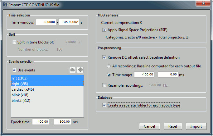
Set the import options as they are represented in this figure:
Time window: Time range of interest. We are interested by all the stimulations, so do not change this parameter; the default values always represent the entire file.
Split: Useful to import continuous recordings without events, to import successive chunks of the same duration. We do not need this here.
Events selection: Check the "Use events" option, and select both "left" and "right". The number in the parenthesis represents the number of occurrences of this event in the selected time window (would change if you modify the time definition on top of the figure)
Epoch time: Time segment that is extracted around each marker and saved in the database. Set it to [-100, +300] ms
Use Signal Space Projections: Use the active SSP projectors calculated during the previous pre-processing steps. Keep this option selected.
Remove DC Offset: Check this option, and select: Time range: [-100, 0] ms. For each epoch, this will: compute the average of each channel over the baseline (pre-stimulus interval: -100ms to 0ms), and subtract it from the channel at every time instants (full epoch interval: [-100,+300]ms).
Resample recordings: Keep this unchecked
Create new conditions for epochs: If selected, a new condition is created for each event type (here, it will create two conditions in the database: "left" and "right"). If not selected, all the epochs are saved in a new folder, the same one for all the events, that has the same name as the initial raw file.
Click on Import and wait. At the end, you are asked whether you want to ignore one epoch that is shorter than the others. This happens because the acquisition of the MEG signals was stopped less than 300ms after the last stimulus trigger was sent. Therefore, the last epoch cannot have the full [-100,300]ms time definition. This shorter epoch would prevent us from averaging all the trials easily. As we already have enough repetitions in this experiment, we can just ignore it. Answer Yes to this question to discard the last epoch.

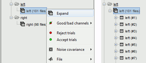
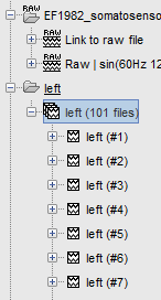
Two new conditions containing two groups of trials appeared in the database. The groups of trials are not expanded by default, in order to have the database tree displayed faster. To expand a list and get access to the individual trials: double click on it, or right-click > Expand.
The SSP projectors calculated in the previous tutorial were applied on the fly when reading from the continuous file. Those epochs are clean from eye blinks and power line contamination.
All the files available in the (Common files) folder are also shared for those new folders "left" and "right".
Review the individual trials
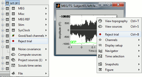
Double-click on the first trial for the "left" condition. Then right-click on the figure > Next data file, or use the keyboard shortcut F3 to jump to the next trial. This way you can quickly review all the trials, to make sure that there is no obvious problem in the recordings. If you haven't reviewed manually all the recordings in the continuous mode, and marked all the bad segments, it is a good time to do it now.
To mark a trial as bad manually, you have three methods:
Right-click on the trial file in the dabase > Reject trial
Right-click on the figure > Reject trial
Use the keyboard shortcut Control+B
To set all the trials back as good in a group: right-click on the trials group or the condition > Accept bad trials.
When a trial is tagged as bad, its icon in the database explorer show a red mark.

All the bad trials are going to be ignored in the rest of the analysis, because they are ignored by the Process1 and Process2 tabs. If you drag and drop the 101 left trials in the Process1 list, with one trial marked as bad, the summary of the selected files on top of the tab would show only 100 data files.

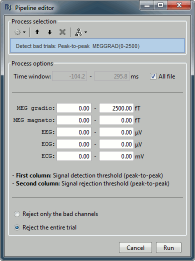
One process can help you detect automatically some bad trials based on a peak-to-peak value threshold. Drag and drop all the trials from the left condition in the Process1 list, and select the process "Artifacts > Detect bad channels: peak-to-peak". For each trial, it detects the channels that have a peak-to-peak amplitude (maximum value - minimum value) that is over a rejection threshold (too noisy) or below a rejection threshold (no signal). You can define different thresholds for different channel types. The options are:
Time window: Time range for which the peak-to-peak value is calculated on each trial
Thresholds: Rejection and detection thresholds for each sensor type. For CTF recordings, use the "MEG gradio" category, and ignore the "/cm (x 0.04)" indication, that is valid only for Neuromag systems. Set the MEG gradio thresholds to [0, 2000] fT, to consider as bad any MEG channel that would have a peak-to-peak amplitude superior to 2000fT.
Reject only the bad channels: This would tag as bad only the detected channels, but would not tag the trial as bad.
Reject the entire trial: This would tag as bad the trial if there is at least one channel file identified as bad.
