|
Size: 8413
Comment:
|
Size: 13004
Comment:
|
| Deletions are marked like this. | Additions are marked like this. |
| Line 4: | Line 4: |
| <<TableOfContents(2)>> | <<TableOfContents(2,2)>> |
| Line 7: | Line 7: |
| 1. Right-click on ''Subject01 / !StimRightThumb / ERP'' > ''Compute sources''.<<BR>><<BR>> {{attachment:popupComputeSources.gif}} --- {{attachment:panelComputeSources.gif}} 1. With this first window you can select the method you want to use to estimate the cortical currents, and the sensors you are going to use for this estimation. The default "Normal mode" only let you edit the following options:<<BR>> |
1. Right-click on ''Subject01 / Right / ERF'' > ''Compute sources''.<<BR>><<BR>> {{attachment:popupComputeSources.gif}} --- {{attachment:panelComputeSources.gif}} 1. With this window you can select the method you want to use to estimate the cortical currents, and the sensors you are going to use for this estimation. The default "Normal mode" only let you edit the following options:<<BR>> |
| Line 10: | Line 10: |
| * '''Method''': No choice, it has to be "Minimum Norm Imaging". All the other methods are less stable and require more pratice. | * '''Method''': Please select wMNE. The other methods dSPM and sLORETA are also based on wMNE. They may give better and/or smoother results depending on the cases. |
| Line 12: | Line 12: |
| * '''Expert mode''': Show many other options we really do not care about right now. This will be explained in another tutorial. | * '''Expert mode''': Show other options we do not care about right now. |
| Line 15: | Line 15: |
| * It is displayed'' inside ''the recordings file ERP, because it is related to this file only. * You can have a look to what there is in the corresponding matrix file (right-click > File > View .mat file). You would find all the options of forward and inverse modelling, and only one interesting field : '''!ImagingKernel''', which contains the inversion kernel. It is a [nVertices x nChannels] matrix that has to be multiplies with the recordings matrix in order to get the activity for each source at all the time samples.<<BR>><<BR>> {{attachment:resultsMat.gif}} |
* It is displayed'' inside ''the recordings file ERF, because it is related to this file only. * Meaning of that weird filename: "MN" stands for "Minimum Norm", and "Constr" stands for "Constrained orientation" of the dipoles (the estimated dipoles orientations are constrained to be normal to the cortex). * You can have a look to the corresponding matrix file (right-click > File > View file contents). You would find all the options of forward and inverse modelling, and only one interesting field : '''!ImagingKernel''', which contains the inversion kernel. It is a [nVertices x nChannels] matrix that has to be multiplied with the recordings matrix in order to get the activity for each source at all the time samples.<<BR>><<BR>> {{attachment:resultsMat.gif}} 1. Do the same for the ''Left / ERF'' file |
| Line 22: | Line 24: |
| 1. Double-click on recordings !StimRightThumb / ERP, to display the time series (always indispensable to have a time reference). 1. Double-click on sources !StimRightThumb / ERP / MN: MEG(Kernel). <<BR>>Equivalent to right-click > Cortical activations > Display on cortex. 1. Go to the main peak around 45ms (by clicking on the times series figure)<<BR>><<BR>> {{attachment:sources1.gif}} 1. Then you can manipulate the sources display exactly the same way as the surfaces and the 2D/3D recodings figures: rotation, zoom, ''Surfaces ''tab(smooth, curvature, resection...), colormap, sensors, pre-defined orientations (keys from 1 to 6)... 1. Only two new controls are available in the ''Surfaces ''tab, in panel ''Data options'': Threshold and transparency. * Transparency: changes the transparency of the sources on the cortex. * Threshold: Only the sources that have a value superior than a given percentage of the colorbar maximum are displayed. |
1. Double-click on recordings ''Right / ERF'', to display the time series (always nice to have a time reference). 1. Double-click on sources ''Right / ERF / MN: MEG''. <<BR>>Equivalent to right-click > Cortical activations > Display on cortex. 1. Go to the main peak around 46ms (by clicking on the times series figure)<<BR>><<BR>> {{attachment:sources1.gif}} 1. Then you can manipulate the sources display exactly the same way as the surfaces and the 2D/3D recordings figures: rotation, zoom, ''Surface ''tab(smoothing, sulci, resection...), colormap, sensors, pre-defined orientations (keys from 0 to 7)... 1. Three new controls are available in the ''Surfaces ''tab, in panel ''Data options'': * '''Amplitude''': Only the sources that have a value superior than a given percentage of the colorbar maximum are displayed. * '''Min. size''': Hide all the small activated regions, ie. the connected color patches that contain a number of vertices smaller than this "min.size" value. * '''Transparency''': Change the transparency of the sources on the cortex. |
| Line 30: | Line 33: |
| * The colorbar maximum depends on the way you configured your ''Sources ''colormap. In case the colormap is NOT normalized to current time frame, and the maximum is NOT set to a specific value, the colorbar maximum should be around 55 pA.m. | * The colorbar maximum depends on the way you configured your ''Sources ''colormap. In case the colormap is NOT normalized to current time frame, and the maximum is NOT set to a specific value, the colorbar maximum should be around 70 pA.m. |
| Line 37: | Line 40: |
| 1. Close all the figures (''Close all'' button). Open the time series view for !StimRightThumb / ERP. 1. Right-click on !StimRightThumb / ERP / MN: MEG(Kernel) > Cortical activations > Display on MRI (3D). 1. This view was also introduced in the tutorial about MRI and surface visualization. Try to rotate, zoom, move the slices, move in time, change the threshold.<<BR>><<BR>> {{attachment:sources3D.gif}} |
1. Close all the figures (''Close all'' button). Open the time series view for Right / ERF. 1. Right-click on Right / ERF / MN: MEG > Cortical activations > Display on MRI (3D). 1. This view was also introduced in the tutorial about MRI and surface visualization. Try to rotate, zoom, move the slices, move in time, change the threshold.<<BR>><<BR>> {{attachment:sources3D.gif}} {{attachment:popupFigMri.gif}} 1. A new menu is available in the popup menu of this figure: MRI Display * '''MIP Anatomy''': for each slice, display the maximum value over all the slices instead of the original value in the strcuctural MRI (fig 1) * '''MIP Functional''': same thing but with the layer of functional values (fig 2) * '''Smooth level''': The sources values are smoothed after being re-interpolated in the volume. Those menus define the size of the smoothing kernel (fig2: smooth=2; fig3: smooth=5).<<BR>><<BR>> {{attachment:mriMipAnat.gif||height="143px",width="176px"}} {{attachment:mriMipFunc.gif||height="142px",width="175px"}} {{attachment:mriSmooth.gif||height="141px",width="173px"}} 1. This view can be used to lots of different types of contact sheets: in time or in space, for each orientation. You can try all the menus. Example: Right-click on the figure > Snapshot > Volume contact sheet: axial: <<BR>><<BR>> {{attachment:popupSnapshot.gif}} {{attachment:contactAxial.gif||height="288px",width="322px"}} |
| Line 42: | Line 50: |
| 1. Right-click on !StimRightThumb / ERP / MN: MEG(Kernel) > Cortical activations > Display on MRI (MRI Viewer). 1. This view was also introduced in the tutorial about MRI and surface visualization. Try to move the slices (sliders, mouse wheel, click on the views), move in time, change the threshold.<<BR>><<BR>> {{attachment:sourcesMriViwer.gif}} |
1. Right-click on Right / ERF / MN: MEG > Cortical activations > Display on MRI (MRI Viewer). 1. This view was also introduced in the tutorial about MRI and surface visualization. Try to move the slices (sliders, mouse wheel, click on the views), move in time, change the threshold.<<BR>><<BR>> {{attachment:sourcesMriViwer.gif||height="331px",width="359px"}} |
| Line 46: | Line 54: |
| The sources file we are observing was computed as an ''inversion kernel''. It means that we can apply it to any similar recordings file (same subject, same run, same positions of sensors). But in our TutorialCTF database, the ''MN: MEG(Kernel)'' node only appears in the the ''ERP ''file, not in the ''Std ''one. What is nessary to share an inversion kernel between different recordings ? | The sources file we are observing was computed as an ''inversion kernel''. It means that we can apply it to any similar recordings file (same subject, same run, same positions of sensors). But in our TutorialCTF database, the ''MN: MEG'' node only appears in the the ''ERF ''file, not in the ''Std ''one. What is nessary to share an inversion kernel between different recordings ? |
| Line 48: | Line 56: |
| 1. Compute another source estimation: but instead of clicking on the ''Compute sources'' fron the ''ERP ''recordings popup menu (which would mean that you only want sources for this particular recordings file), get this menu from the ''!StimRightThumb'' condition. This means that you want the inversion model to be applied to all the data in the condition.<<BR>><<BR>> {{attachment:popupComputeMulti.gif}} | 1. Compute another source estimation: but instead of clicking on the ''Compute sources'' fron the ''ERF ''recordings popup menu (which would mean that you only want sources for this particular recordings file), get this menu from the ''Right''''' condition'''. This means that you want the inversion model to be applied to all the data in the condition. |
| Line 52: | Line 60: |
| 1. Three new nodes are available in the tree:<<BR>><<BR>> {{attachment:treeMinNormMulti.gif}} | 1. Three new nodes are available in the tree:<<BR>><<BR>> {{attachment:popupComputeMulti.gif}} {{attachment:treeMinNormMulti.gif}} |
| Line 54: | Line 62: |
| 1. The actual inversion kernel you have just computed (1), which contains the same information as the one from the previous section (Computing sources for a single data file). Note that you cannot do anything with this file: if you right-click on it, you will see that there are no ''Display ''menu for it. * Two links (2 and 3) that allow you apply this inversion kernel to the data files available in this condition (''ERP ''and ''Std''). In their popup menus, there are all the display options introduced in the previous section. |
1. The actual inversion kernel you have just computed (1), contains the same information as the one from the previous section (Computing sources for a single data file). Note that you cannot do anything with this file: if you right-click on it, you can see that there are no ''Display ''menu for it. * Two links (2) that allow you apply this inversion kernel to the data files available in this condition (''ERF ''and ''Std''). In their popup menus, there are all the display options introduced in the previous section. |
| Line 57: | Line 65: |
| * Right-click on the link in ERP (2) > File > View .mat file. The fields points to the recordings file (!DataFile) and the inversion kernel file (!LinkToFile). When you request any operation on this file, both recordings and kernel are loaded, multiplied to get the sources values, and then processed. <<BR>><<BR>> {{attachment:linkresultsMat.gif}} * The sources for the ''Std ''file do not have any meaning (it contains information about the averaging); but it illustrates the way a kernel is shared |
* Those links are not saved as files but as specific strings in the database: "link|kernel_file|data_file". This means that to represent them, one should load the shared kernel, load the recordings, and multiply them. * The sources for the ''Std ''file do not have any meaning, do not even try to open it. It was just to illustrate the way a kernel is shared |
| Line 60: | Line 68: |
| 1. Double-click on both sources files available for StimRightThumb/ERP, and check at many different times that the cortical maps are exactly the same in both cases. | 1. Double-click on both sources files available for ''Right / ERF'' (link and non-link), and verify at many different times that the cortical maps are exactly the same in both cases. |
| Line 65: | Line 73: |
| == Minimum norm options == Let's introduce briefly the other options offered for the source estimation. Right-click again on Right / ERF > Compute sources. Click on "Expert mode", you more options appearing in the window.If you click on Run, you have access to all the options of the wMNE algorithm. {{attachment:panelExpert.gif}} {{attachment:panelOptions.gif}} === Method === * '''wMNE''': Linear L2-minimum norm estimates algorithm inspired from Matti Hamalainen's MNE software. Introduced in Brainstorm 3.1 by Rey Ramirez. For a full description of this method, please refer to the MNE manual, section 6, "The current estimates". [[http://www.nmr.mgh.harvard.edu/meg/manuals/MNE-manual-2.7.pdf|Download MNE manual here]]. * '''dSPM''': Noise-normalized estimate (dynamical Statistical Parametric Mapping). Its computation is based on the wMNE solution. * '''sLORETA''': Noise-normalized estimate using the sLORETA approach. sLORETA solutions have in general a smaller location bias than either the expected current (MNE) or the dSPM. * '''Old minimum norm''': Minimum norm solution from Brainstorm 3 and earlier. For compatibility purpose only. * '''Cortical LCMV beamformer''': Ongoing development. Not stable enough yet. === Output mode === * '''Full results''': Saves in one big matrix the values of all the sources (15000) for all the time samples (375). * The size in memory of such a matrix is about 45Mb for 300ms of recordings. This is still reasonable, so you may use this option in this case. But if you need to process longer recordings, you may have some "Out of memory" errors in Matlab, or fill your hard drive quickly. * '''Kernel only''': Saves only the ''Inversion kernel'', a matrix that describes how to compute the sources when you know the values at the sensor level. So its size is: number of sources (15000) x number of sensors (151). * To get the sources time series, you just need to multiply this kernel by the MEG recordings. * '''Full results '''=''' Inversion kernel '''*''' Recordings''' * The size of this matrix is about 18Mb. In this case, the difference is not very important because we only process 375 time samples. But this inversion kernel is independent from the recordings length, so you can easily scale its computation to much longer recordings. * This is possible because those minimum norm methods are linear methods. * Which option should you choose ? * Probably "''Kernel only''", as it is faster and produces smaller files. * All the following operations in Brainstorm will be exactly the same whatever you select. Each time you access the sources values, the program has to do the multiplication Kernel * Recordings, but this is done in a totally transparent way. * The only reason that would make you chose the "''Full results''" options would be any interest in having the full matrix in one file, in case you want to process the sources values by yourself (filtering, statistics, display...). === Source orientation === * '''Constrained''': * '''Loose''': * '''Unconstrained''': * '''Truncated''': === Signal properties === * '''Signal to noise ratio (SNR)''': * '''PCA Whitening''': === Noise covariance matrix === * '''Full noise covariance''': * '''Diagonal noise covariance''': * '''Regularize noise covariance''': === Depth weighting === |
Tutorial 7: Source estimation
Now you have in your database a forward model matrix that explains how the cortical sources determine the values on the sensors. This is useful for simulations, but what we really need is to build the inverse information: how to estimate the sources when you have the recordings. Many solutions are described in the literature, some of them are implemented in Brainstorm, and only one is presented in this tutorial: the minimum-norm estimation. It is not really the most advanced solution, but it is one of the most robust.
Contents
Computing sources for a single data file
Right-click on Subject01 / Right / ERF > Compute sources.
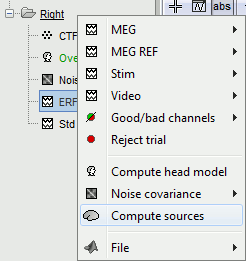 ---
--- 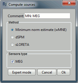
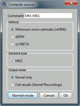
With this window you can select the method you want to use to estimate the cortical currents, and the sensors you are going to use for this estimation. The default "Normal mode" only let you edit the following options:
Comment: This field contains what is going to be displayed in the database explorer.
Method: Please select wMNE. The other methods dSPM and sLORETA are also based on wMNE. They may give better and/or smoother results depending on the cases.
Sensors type: Modalities that are used for the reconstruction. Here we only have one type of MEG sensors (axial gradiometers), so nothing to change.
Expert mode: Show other options we do not care about right now.
- Click on Run.
A new file is available in the database explorer.
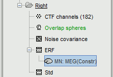
It is displayed inside the recordings file ERF, because it is related to this file only.
- Meaning of that weird filename: "MN" stands for "Minimum Norm", and "Constr" stands for "Constrained orientation" of the dipoles (the estimated dipoles orientations are constrained to be normal to the cortex).
You can have a look to the corresponding matrix file (right-click > File > View file contents). You would find all the options of forward and inverse modelling, and only one interesting field : ImagingKernel, which contains the inversion kernel. It is a [nVertices x nChannels] matrix that has to be multiplied with the recordings matrix in order to get the activity for each source at all the time samples.
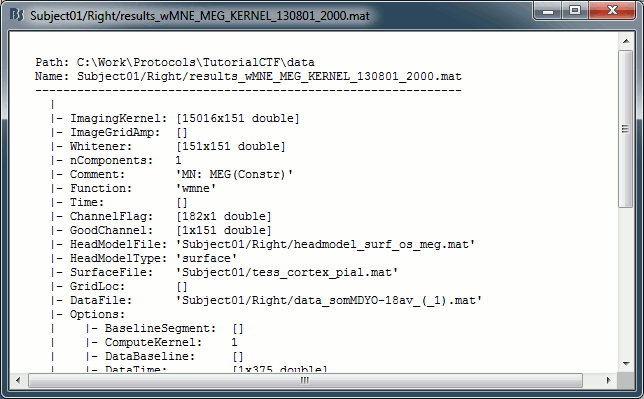
Do the same for the Left / ERF file
Sources visualization
There are two main ways to display the sources: on the cortex surface and on the MRI slices.
Sources on cortex surface
Double-click on recordings Right / ERF, to display the time series (always nice to have a time reference).
Double-click on sources Right / ERF / MN: MEG.
Equivalent to right-click > Cortical activations > Display on cortex.Go to the main peak around 46ms (by clicking on the times series figure)
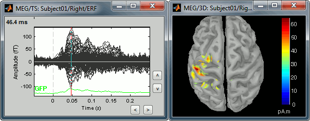
Then you can manipulate the sources display exactly the same way as the surfaces and the 2D/3D recordings figures: rotation, zoom, Surface tab(smoothing, sulci, resection...), colormap, sensors, pre-defined orientations (keys from 0 to 7)...
Three new controls are available in the Surfaces tab, in panel Data options:
Amplitude: Only the sources that have a value superior than a given percentage of the colorbar maximum are displayed.
Min. size: Hide all the small activated regions, ie. the connected color patches that contain a number of vertices smaller than this "min.size" value.
Transparency: Change the transparency of the sources on the cortex.
Take a few minutes to understand what this threshold value represents.
The colorbar maximum depends on the way you configured your Sources colormap. In case the colormap is NOT normalized to current time frame, and the maximum is NOT set to a specific value, the colorbar maximum should be around 70 pA.m.
- On the screenshot above, the threshold value was set to 34%. It means that only the sources that had a value over 0.34*55 = 18.7 pA.m were visible.
- If you set the threshold to 0%, you display all the sources values on the cortex surface; and as most of the sources have values close to 0, the brain is mainly blue.
Move the slider and look for a threshold value that would give you a really focal source.The following figures represent the sources activations at t=46ms respectively with threshold at 0% and 90%.
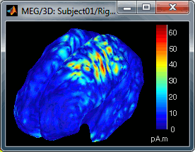
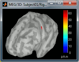
- The figure on the right shows the most active area of the cortex 46ms after an electric stimulation of the right thumb. As expected, it is localized in the left hemisphere, in the middle of post central gyrus (projection of the right hand in the primary somatosensory cortex).
Sources on MRI (3D)
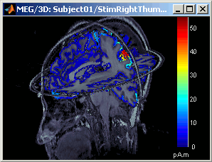
Close all the figures (Close all button). Open the time series view for Right / ERF.
Right-click on Right / ERF / MN: MEG > Cortical activations > Display on MRI (3D).
This view was also introduced in the tutorial about MRI and surface visualization. Try to rotate, zoom, move the slices, move in time, change the threshold.
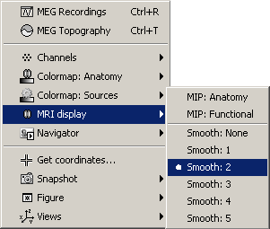
- A new menu is available in the popup menu of this figure: MRI Display
MIP Anatomy: for each slice, display the maximum value over all the slices instead of the original value in the strcuctural MRI (fig 1)
MIP Functional: same thing but with the layer of functional values (fig 2)
Smooth level: The sources values are smoothed after being re-interpolated in the volume. Those menus define the size of the smoothing kernel (fig2: smooth=2; fig3: smooth=5).
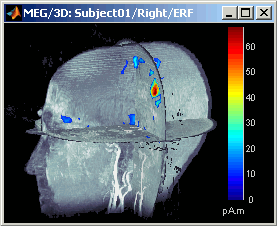
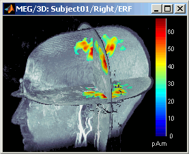
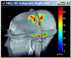
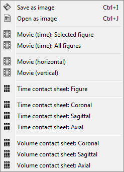
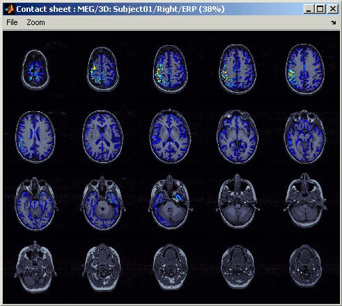
This view can be used to lots of different types of contact sheets: in time or in space, for each orientation. You can try all the menus. Example: Right-click on the figure > Snapshot > Volume contact sheet: axial:
Sources on MRI (MRI Viewer)
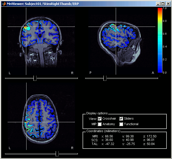
Right-click on Right / ERF / MN: MEG > Cortical activations > Display on MRI (MRI Viewer).
This view was also introduced in the tutorial about MRI and surface visualization. Try to move the slices (sliders, mouse wheel, click on the views), move in time, change the threshold.
Computing sources for multiple data files
The sources file we are observing was computed as an inversion kernel. It means that we can apply it to any similar recordings file (same subject, same run, same positions of sensors). But in our TutorialCTF database, the MN: MEG node only appears in the the ERF file, not in the Std one. What is nessary to share an inversion kernel between different recordings ?
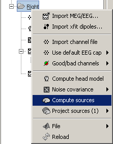
Compute another source estimation: but instead of clicking on the Compute sources fron the ERF recordings popup menu (which would mean that you only want sources for this particular recordings file), get this menu from the Right condition. This means that you want the inversion model to be applied to all the data in the condition.
- Select "Minimum Norm Imaging", click on Run.
Three new nodes are available in the tree:
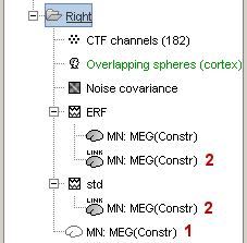
The actual inversion kernel you have just computed (1), contains the same information as the one from the previous section (Computing sources for a single data file). Note that you cannot do anything with this file: if you right-click on it, you can see that there are no Display menu for it.
Two links (2) that allow you apply this inversion kernel to the data files available in this condition (ERF and Std). In their popup menus, there are all the display options introduced in the previous section.
- Those links are not saved as files but as specific strings in the database: "link|kernel_file|data_file". This means that to represent them, one should load the shared kernel, load the recordings, and multiply them.
The sources for the Std file do not have any meaning, do not even try to open it. It was just to illustrate the way a kernel is shared
Double-click on both sources files available for Right / ERF (link and non-link), and verify at many different times that the cortical maps are exactly the same in both cases.
You can estimate the sources for many subjects or conditions at once, as it was explained for the head models in previous tutorial: the Compute sources menu is available on all the subjects and conditions popup menus.
- Delete the shared kernel (1), we don't need redundant and confusing information for the next steps. Observe that both links disappear at the same time.
Minimum norm options
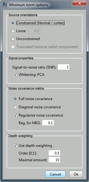
Let's introduce briefly the other options offered for the source estimation. Right-click again on Right / ERF > Compute sources. Click on "Expert mode", you more options appearing in the window.If you click on Run, you have access to all the options of the wMNE algorithm.
Method
wMNE: Linear L2-minimum norm estimates algorithm inspired from Matti Hamalainen's MNE software. Introduced in Brainstorm 3.1 by Rey Ramirez. For a full description of this method, please refer to the MNE manual, section 6, "The current estimates". Download MNE manual here.
dSPM: Noise-normalized estimate (dynamical Statistical Parametric Mapping). Its computation is based on the wMNE solution.
sLORETA: Noise-normalized estimate using the sLORETA approach. sLORETA solutions have in general a smaller location bias than either the expected current (MNE) or the dSPM.
Old minimum norm: Minimum norm solution from Brainstorm 3 and earlier. For compatibility purpose only.
Cortical LCMV beamformer: Ongoing development. Not stable enough yet.
Output mode
Full results: Saves in one big matrix the values of all the sources (15000) for all the time samples (375).
- The size in memory of such a matrix is about 45Mb for 300ms of recordings. This is still reasonable, so you may use this option in this case. But if you need to process longer recordings, you may have some "Out of memory" errors in Matlab, or fill your hard drive quickly.
Kernel only: Saves only the Inversion kernel, a matrix that describes how to compute the sources when you know the values at the sensor level. So its size is: number of sources (15000) x number of sensors (151).
- To get the sources time series, you just need to multiply this kernel by the MEG recordings.
Full results = Inversion kernel * Recordings
- The size of this matrix is about 18Mb. In this case, the difference is not very important because we only process 375 time samples. But this inversion kernel is independent from the recordings length, so you can easily scale its computation to much longer recordings.
- This is possible because those minimum norm methods are linear methods.
- Which option should you choose ?
Probably "Kernel only", as it is faster and produces smaller files.
- All the following operations in Brainstorm will be exactly the same whatever you select. Each time you access the sources values, the program has to do the multiplication Kernel * Recordings, but this is done in a totally transparent way.
The only reason that would make you chose the "Full results" options would be any interest in having the full matrix in one file, in case you want to process the sources values by yourself (filtering, statistics, display...).
Source orientation
Constrained:
Loose:
Unconstrained:
Truncated:
Signal properties
Signal to noise ratio (SNR):
PCA Whitening:
Noise covariance matrix
Full noise covariance:
Diagonal noise covariance:
Regularize noise covariance:
Depth weighting
Next
You can now observe the cortical maps estimated from a MEG evoked potential. This information is interesting in itself, but it is an image; it is difficult to compare it rigorously with other subjects or stimulations, or to test statistically some hypothesis.
The next tutorial describes how to create and study a ?region of interest.
