|
Size: 4196
Comment:
|
Size: 11355
Comment:
|
| Deletions are marked like this. | Additions are marked like this. |
| Line 1: | Line 1: |
| ## page was renamed from Tutorials/TutSourcesEstimation | |
| Line 36: | Line 35: |
| 1. A new file is available in the database explorer. | 1. A new file is available in the database explorer.<<BR>><<BR>> {{attachment:treeMinNorm.gif}} |
| Line 38: | Line 37: |
| * You can have a look to what there is in the corresponding matrix file (right-click > File > View .mat file). You would find all the options of forward and inverse modelling, and only one interesting field : '''ImagingKernel'''. | * You can have a look to what there is in the corresponding matrix file (right-click > File > View .mat file). You would find all the options of forward and inverse modelling, and only one interesting field : '''!ImagingKernel'''. == Sources visualization == There are two main ways to display the sources: on the cortex surface and on the MRI slices. === Sources on cortex surface === 1. Double-click on recordings !StimRightThumb / ERP, to display the time series (always indispensable to have a time reference). 1. Double-click on sources !StimRightThumb / ERP / MN: MEG(Kernel). <<BR>>Equivalent to right-click > Cortical activations > Display on cortex. 1. Go to the main peak around 45ms (by clicking on the times series figure)<<BR>><<BR>> {{attachment:sources1.gif}} 1. Then you can manipulate the sources display exactly the same way as the surfaces and the 2D/3D recodings figures: rotation, zoom, ''Surfaces ''tab(smooth, curvature, resection...), colormap, sensors, pre-defined orientations (keys from 1 to 6)... 1. Only two new controls are available in the ''Surfaces ''tab, in panel ''Data options'': Threshold and transparency. * Transparency: changes the transparency of the sources on the cortex. * Threshold: Only the sources that have a value superior than a given percentage of the colorbar maximum are displayed. 1. Take a few minutes to understand what this threshold value represents.<<BR>> * The colorbar maximum depends on the way you configured your ''Sources ''colormap. In case the colormap is NOT normalized to current time frame, and the maximum is NOT set to a specific value, the colorbar maximum should be around 55 pA.m. * On the screenshot above, the threshold value was set to 34%. It means that only the sources that had a value over 0.34*55 = 18.7 pA.m were visible. * If you set the threshold to 0%, you display all the sources values on the cortex surface; and as most of the sources have values close to 0, the brain is mainly blue. * Move the slider and look for a threshold value that would give you a really focal source.The following figures represent the sources activations at t=46ms respectively with threshold at 0% and 90%.<<BR>><<BR>> {{attachment:threshold0.gif}} {{attachment:threshold90.gif}} * The figure on the right shows the most active area of the cortex 46ms after an electric stimulation of the right thumb. As expected, it is localized in the middle of post central gyrus (projection of the hand in the primary somatosensory cortex). === Sources on MRI === 1. Close all the figures (''Close all'' button). Open the time series view for !StimRightThumb / ERP. 1. Right-click on !StimRightThumb / ERP / MN: MEG(Kernel) > Cortical activations > Display on MRI (3D). 1. This view was also introduced in the tutorial about MRI and surface visualization. Try to rotate, zoom, move the slices, move in time, change the threshold.<<BR>><<BR>> {{attachment:sources3D.gif}} === Modelized data === What is called ''modelized data ''here is the part of the recordings that are explained by the minimum-norm solution. This information is saved the sources file, in the ''Fsynth ''field. 1. Close all the figures. Open the'' 2D sensor cap'' view for !StimRightThumb / ERP. 1. Right-click on ERP sources file > Modelized data > Display time series 1. Right-click on ERP sources file > Modelized data > 2D sensor cap 1. You can browse among time to observe what are the differences between what the model explains and the real recordings. The modelized data is smoother: the regularization which is applied to obtain the sources is supposed to lower the noise.<<BR>><<BR>>''' {{attachment:topoReal.gif}} {{attachment:topoModelized.gif}} ''' === Residuals === The ''residuals ''are the difference between the recordings and the modelized data. This information is not stored in any file but reconstructed when needed. 1. Right-click on ERP sources > Residuals > Display time series<<BR>>At each time: Residuals = || Modelized - Recordings || / || max(Recordings) 1. Right-click on ERP sources > Residuals > 2D sensor cap: Spatial representation of the same values. 1. Right-click on ERP sources > Residuals > Display global error:<<BR>>At each time: Norm of residuals across all the sensors / Norm of the recordings across all the sensors<<BR>><<BR>>''' {{attachment:residualsTS.gif|residualsTopo.gif|height="163",width="216"}} {{attachment:residualsTopo.gif||height="162",width="212"}} {{attachment:residualsGlobal.gif||height="162",width="215"}} ''' == Computing sources for multiple data files == The sources file we are observing was computed as am ''inversion kernel''. It means that we can apply it to any similar recordings file (same subject, same run, same positions of sensors). But in our TutorialCTF database, the ''MN: MEG(Kernel)'' node only appears in the the ERP file, not in the Std one. What is nessary to share an inversion kernel between different recordings ? 1. Compute another source estimation: but instead of clicking on the ''Compute sources'' fron the ''ERP ''recordings popup menu (which would mean that you only want sources for this particular recordings file), get this menu from the ''!StimRightThumb'' condition. This means that you want the inversion model to be applied to all the data in the condition.<<BR>><<BR>> {{attachment:popupComputeMulti.gif}} 1. Select "Min. Norm Imaging", click Run, and then click Ok to validate the default options for minimum norm estimation. 1. Three new nodes are available in the tree:<<BR>><<BR>> {{attachment:treeMinNormMulti.gif}} 1. The actual inversion kernel you have just computed (1), which contains the same information as the one from the previous section (Computing sources for a single data file). Note that you cannot do anything with this file: if you right-click on it, you will see that there are no ''Display ''menu for it. * Two links (2 and 3) that allow you apply this inversion kernel to the data files available in this condition (''ERP ''and ''Std''). In their popup menus, there are all the display options introduced in the previous section. * Right-click on the link in ERP (2) > File > View .mat file. The fields points to the recordings file (!DataFile) and the inversion kernel file (!LinkToFile). When you request any operation on this file, both recordings and kernel are loaded, multiplied to get the sources values, and then processed. <<BR>><<BR>> {{attachment:linkresultsMat.gif}} * The sources for the ''Std ''file do not have any meaning (it contains information about the averaging); but it illustrates the way a kernel is shared 1. Double-click on both sources files available for StimRightThumb/ERP, and check at many different times that the cortical maps are exactly the same in both cases. 1. Delete the shared kernel (1), we don't need redundant and confusing information for the next steps. And observe that both links disappear at the same time. == Next == You can now observe the cortical maps estimated from a MEG evoked potential. This information is interesting in itself, but it is an image; it is difficult to compare it rigorously with other subjects or stimulations, or to test statistically some hypothesis. The next tutorial describes how to create and study some [[Tutorials/TutScouts|regions of interest]]. |
Tutorial: Source estimation
This tutorial is still based on Sabine Meunier's somatotopy experiment, called TutorialCTF in your Brainstorm database.
Now you have in you database a forward model matrix that explains how the cortical sources determine the values on the sensors. This is useful for simulations, but what we really need is to build the inverse information: how to estimate the sources when you have the results. Many solutions described in the literature, some of them are implemented in Brainstorm, and only one is presented in this tutorial: the minimum-norm estimation. It is not really the most advanced solution, but it is one of the most robust.
For more information about inverse models and minimum-norm estimation, visit the ?Theory section.
Contents
Computing sources for a single data file
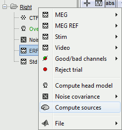
Right-click on Subject01 / StimRightThumb / ERP > Compute sources.
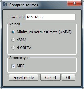
- With this first window you can select the method you want to use to estimate the cortical currents, and the sensors you are going to use for this estimation.
- Edit the Comment field if you want.
- Select "Min. Norm Imaging"
- For the sensors, you have no other option than MEG (All), because those recordings were recorded with only one type of MEG sensors (axial gradiometers) and no EEG signal was registrated at the same time.
- Run.
The next window shows the options for the minimum norm estimation algorithm.
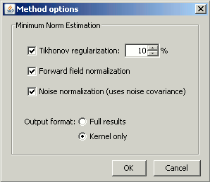
Leave the Tikhonov and Forward field normalization selected. To learn more about those options, please consult the the ?Theory section.
However, you need to understand well what is the meaning of the last option, Output format, which defines the way the sources estimates are saved.
Full results: Saves in one big matrix the values of all the sources (15000) for all the time samples (375).
- The size in memory of such a matrix is about 45Mb for 300ms of recordings. This is still reasonable, so you may use this option in this case.
- But if you need to process longer recordings, you may have some "Out of memory" errors in Matlab, or fill your hard drive quicklky.
Kernel only: Saves only the Inversion kernel, a matrix which describes how to compute the sources when you know the values at the sensors level. So its size is: number of sources (15000) x number of sensors (151).
- To get the sources time series, you just need to multiply this kernel by the MEG recordings.
Full results = Inversion kernel * Recordings
- The size of this matrix is about 18Mb. In this case, the difference is not very important because we only process 375 time samples. But this inversion kernel is independent from the recordings length, so you can easily scale its computation to much longer recordings.
- This is possible because the Minimum norm estimation is a linear method.
- Which option should you choose ?
Probably "Kernel only", as it is faster and produces smaller files.
- All the following operations in Brainstorm will be exactly the same whatever you select. Each time you will access the sources values, the program will have to do the multiplication Kernel * Recordings, but this is done in a totally transparent way.
The only reason that would make you chose the "Full results" options would be any interest in having the full matrix in one file, in case you want to process the sources values by yourself (filtering, statistics, display...).
So please "Kernel only" for the moment. And click Ok.
A new file is available in the database explorer.
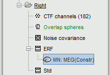
It is displayed inside the recordings file ERP, because it is related to this file only.
You can have a look to what there is in the corresponding matrix file (right-click > File > View .mat file). You would find all the options of forward and inverse modelling, and only one interesting field : ImagingKernel.
Sources visualization
There are two main ways to display the sources: on the cortex surface and on the MRI slices.
Sources on cortex surface
Double-click on recordings StimRightThumb / ERP, to display the time series (always indispensable to have a time reference).
Double-click on sources StimRightThumb / ERP / MN: MEG(Kernel).
Equivalent to right-click > Cortical activations > Display on cortex.Go to the main peak around 45ms (by clicking on the times series figure)
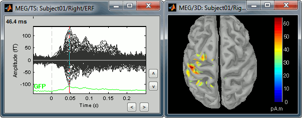
Then you can manipulate the sources display exactly the same way as the surfaces and the 2D/3D recodings figures: rotation, zoom, Surfaces tab(smooth, curvature, resection...), colormap, sensors, pre-defined orientations (keys from 1 to 6)...
Only two new controls are available in the Surfaces tab, in panel Data options: Threshold and transparency.
- Transparency: changes the transparency of the sources on the cortex.
- Threshold: Only the sources that have a value superior than a given percentage of the colorbar maximum are displayed.
Take a few minutes to understand what this threshold value represents.
The colorbar maximum depends on the way you configured your Sources colormap. In case the colormap is NOT normalized to current time frame, and the maximum is NOT set to a specific value, the colorbar maximum should be around 55 pA.m.
- On the screenshot above, the threshold value was set to 34%. It means that only the sources that had a value over 0.34*55 = 18.7 pA.m were visible.
- If you set the threshold to 0%, you display all the sources values on the cortex surface; and as most of the sources have values close to 0, the brain is mainly blue.
Move the slider and look for a threshold value that would give you a really focal source.The following figures represent the sources activations at t=46ms respectively with threshold at 0% and 90%.
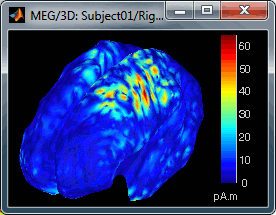
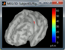
- The figure on the right shows the most active area of the cortex 46ms after an electric stimulation of the right thumb. As expected, it is localized in the middle of post central gyrus (projection of the hand in the primary somatosensory cortex).
Sources on MRI
Close all the figures (Close all button). Open the time series view for StimRightThumb / ERP.
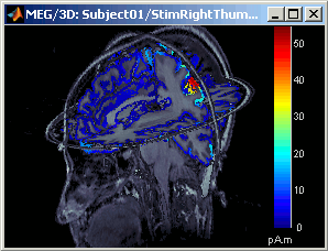
Right-click on StimRightThumb / ERP / MN: MEG(Kernel) > Cortical activations > Display on MRI (3D).
This view was also introduced in the tutorial about MRI and surface visualization. Try to rotate, zoom, move the slices, move in time, change the threshold.
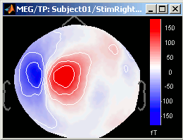
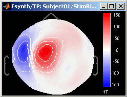
Modelized data
What is called modelized data here is the part of the recordings that are explained by the minimum-norm solution. This information is saved the sources file, in the Fsynth field.
Close all the figures. Open the 2D sensor cap view for StimRightThumb / ERP.
Right-click on ERP sources file > Modelized data > Display time series
Right-click on ERP sources file > Modelized data > 2D sensor cap
You can browse among time to observe what are the differences between what the model explains and the real recordings. The modelized data is smoother: the regularization which is applied to obtain the sources is supposed to lower the noise.
Residuals
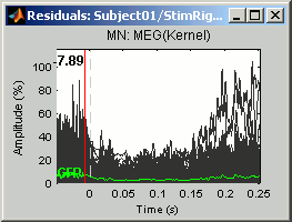
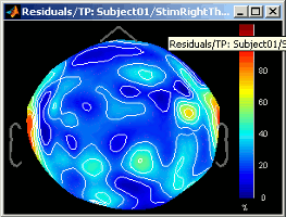
The residuals are the difference between the recordings and the modelized data. This information is not stored in any file but reconstructed when needed.
Right-click on ERP sources > Residuals > Display time series
At each time: Residuals = || Modelized - Recordings || / || max(Recordings)Right-click on ERP sources > Residuals > 2D sensor cap: Spatial representation of the same values.
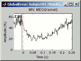
Right-click on ERP sources > Residuals > Display global error:
At each time: Norm of residuals across all the sensors / Norm of the recordings across all the sensors
Computing sources for multiple data files
The sources file we are observing was computed as am inversion kernel. It means that we can apply it to any similar recordings file (same subject, same run, same positions of sensors). But in our TutorialCTF database, the MN: MEG(Kernel) node only appears in the the ERP file, not in the Std one. What is nessary to share an inversion kernel between different recordings ?
Compute another source estimation: but instead of clicking on the Compute sources fron the ERP recordings popup menu (which would mean that you only want sources for this particular recordings file), get this menu from the StimRightThumb condition. This means that you want the inversion model to be applied to all the data in the condition.
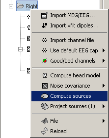
- Select "Min. Norm Imaging", click Run, and then click Ok to validate the default options for minimum norm estimation.
Three new nodes are available in the tree:
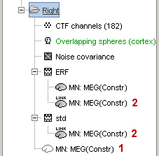
The actual inversion kernel you have just computed (1), which contains the same information as the one from the previous section (Computing sources for a single data file). Note that you cannot do anything with this file: if you right-click on it, you will see that there are no Display menu for it.
Two links (2 and 3) that allow you apply this inversion kernel to the data files available in this condition (ERP and Std). In their popup menus, there are all the display options introduced in the previous section.
Right-click on the link in ERP (2) > File > View .mat file. The fields points to the recordings file (DataFile) and the inversion kernel file (LinkToFile). When you request any operation on this file, both recordings and kernel are loaded, multiplied to get the sources values, and then processed.
![[ATTACH] [ATTACH]](/moin_static1911/brainstorm1/img/attach.png)
The sources for the Std file do not have any meaning (it contains information about the averaging); but it illustrates the way a kernel is shared
- Double-click on both sources files available for StimRightThumb/ERP, and check at many different times that the cortical maps are exactly the same in both cases.
- Delete the shared kernel (1), we don't need redundant and confusing information for the next steps. And observe that both links disappear at the same time.
Next
You can now observe the cortical maps estimated from a MEG evoked potential. This information is interesting in itself, but it is an image; it is difficult to compare it rigorously with other subjects or stimulations, or to test statistically some hypothesis.
The next tutorial describes how to create and study some ?regions of interest.
