|
Size: 33181
Comment:
|
Size: 35184
Comment:
|
| Deletions are marked like this. | Additions are marked like this. |
| Line 22: | Line 22: |
| From the figure above, which designs the Morlet wavelet, we can see that the default wavelet (central frequency 1Hz, FWHM=3sec) has temporal resolution 0.60sec at 5Hz and 0.3sec at 10Hz. In such case, the edge effects are roughly half these times: 0.30sec in 5Hz and 0.15sec in 10Hz. Examples of such edge effects are given in the figures below. | From the figure above, which designs the Morlet wavelet, we can see that the default wavelet (central frequency 1Hz, FWHM=3sec) has temporal resolution 0.25sec at 5Hz and 0.1sec at 10Hz. In such case, the edge effects are roughly half these times: 125ms in 5Hz and 50ms in 10Hz. Examples of such edge effects are given in the figures below. |
| Line 26: | Line 26: |
| == TF: Recordings == * We are going first to compute the time-frequency decomposition for the two averaged recordings we have in the protocol. * Drag'n'drop the two ERF files from ''Right ''and ''Left ''in ''Process1''. Select "Recordings".<<BR>><<BR>> {{attachment:fileSelection.gif}} * Click on Run. Select the process: Analyze > Time-frequency decomposition. You do not have anything else to configure here. Click on Ok.<<BR>><<BR>> {{attachment:processSelection.gif}} * Time-frequency option window. You may: 1) define bands in time and frequency or analyze the data in all points, 2) configure the time and frequency resolution of the wavelets, 3) define which sensors to process, and the output type (complex coefficients or squared coefficients / power). <<BR>><<BR>> {{attachment:timeFreqOptionsBasic.gif}} |
== Time-frequency decomposition of MEG Recordings == We are going first to compute the time-frequency decomposition for the two averaged recordings we have in the protocol. Drag'n'drop the two ERF files from ''Right ''and ''Left ''in ''Process1''. Select "Recordings". {{attachment:fileSelection.gif}} Click on Run. Select the process: '''Frequency > Time-frequency (Morlet wavelets)'''. * The only generic option you have access to in this window is the selection of the sensors on which you want to apply the process. You can use this box to select a mixed list of channel types (ex: "MEG") or channel names (ex: "MRT16"). * For now, you can just leave the default "MEG, EEG". There is no EEG channel but it doesn't matter, the extra information is just ignored. Click on the "Edit" button to get access to the options specific to the time-frequency decomposition process. {{attachment:processSelection.gif}} Time-frequency option window. You may: 1. define bands in time and frequency or analyze the data in all points, 1. configure the time and frequency resolution of the wavelets, 1. define the output type (complex coefficients or squared coefficients / power). {{attachment:timeFreqOptionsBasic.gif}} |
| Line 33: | Line 49: |
| * '''Comment''': This is the string that will be displayed in the database explorer to represent the output file. * '''Time definition''': * This panel describes the time points for which you will get a value at the end of the computation. * '''Same as input file''': If you select this option, you would get the time-frequency decomposition (TF) for each of the time samples in the input file (here: 375 samples between -50ms to 250ms) * '''Group in time bands''': This option adds another step of computation: * 1) It first computes the TF for each of the time points in the initial file, exactly like with the "same as input file" option * 2) For each time band: it groups the corresponding time points by averaging the power of their TF values. * Definition of the time bands: two methods * Enter your own time bands in the text area, one line per time band, with following format: "name : start_time, stop_time" * Click on the "Generate" button to create automatically a list of time bands with the same length. You will be asked the maximal length of each time band. * '''Frequency definition''': * This panel describes the frequencies for which the power will be estimated at each time instant. * '''Linear''': You can specify the frequencies with any Matlab syntax start:step:stop. The default is "1:1:30", which produces 60 values [1, 2, 3, 4, ..., 59, 60] * '''Group in frequency bands''': As for the time definition, this option leads to a two-step process: * 1) It computes the TF for 4 frequencies for each frequency band. For example, the first default frequency band "delta: 2,4" would estimate the TF for the frequencies [2, 2.66, 3.33, 4] * 2) Then for each frequency band: it averages the power of the 4 frequencies, so that you get only one value for each frequency band (and for each time point and each sensor). * Definition of the frequency bands: * One line per frequency band, with the format "name : start_freq, stop_freq" * Click on the "Reset" button to go back to the default settings. * '''Morlet wavelet options''': * Central frequency: frequency where the mother wavelet is designed. All other wavelets will be shifted and scaled versions of the mother wavelet * Time resolution (FWHM): desirable temporal resolution of the wavelet at the central frequency (in units of Full Width Half Maximum). Click 'display' to see the resolution of the wavelet in other frequencies * See the first section of this tutorial for a description of those parameters. * '''Processing options''': * '''Sensors to process''': * This is the list of the sensors for which the TF is going to be computed. * You can provide either sensor types (eg. EEG, MEG, MEG GRAD), or sensor names (eg. MLC15, MEG0121, EEG23) * '''Compute the following measure''': * The TF returns basically the wavelet coefficients for each frequency/time/sensor, which are complex values. Typically, what you want to display is the power of the coefficients, which is the square of the amplitude: abs(TF).^2. You can choose if you want to apply this transformation or not. * '''Power''': Applies the "power" transformation right after the computation. This causes a loss of the phase information. * '''None''': Save the TF coefficients as they are computed. This can be useful if you plan to use those decompositions for other purposes that require the phase. * If you select "None" here, the power will be computed on the fly for the various displays. * Some combinations of options may disable this choice. Example: if you ask for time bands or frequency bands, the program will have to compute the power before averaging the values; so in those cases the "None" option is disabled. * '''Output''': * '''Save individual TF maps''': This option stops the computation here, and saves in the database one time-frequency file for each input file. * Be very careful using this option because if you have hundreds of trials, it will fill your hard drive very quickly. * One full TF file in this case contains [nSensors x nTime x nFreq] = 3.397.500 values = 25 Mb. * You can however limit the amount of data produced by using time and/or frequency bands. For 15 time bands and 6 frequency bands, the size of each file drops to: 110 Kb. * '''Save average TF maps''': This option is available only when there are more than one input files (number of files you dropped in the Processes tab). * Instead of saving the TF for each file separately, it automatically computes the average of the power of all the TF. * This is a good choice if you do not plan to use independently all the TF files, because it saves a lot of time and disk space. |
'''Comment''': String that will be displayed in the database explorer to represent the output file. '''Time definition''': * This panel describes the time points for which you will get a value at the end of the computation. * '''Same as input file''': If you select this option, you would get the time-frequency decomposition (TF) for each of the time samples in the input file (here: 375 samples between -50ms to 250ms) * '''Group in time bands''': This option adds another step of computation: * It first computes the TF for each of the time points in the initial file, exactly like with the "same as input file" option * Then for each time band: it groups the corresponding time points by averaging the power of their TF values. * Definition of the time bands: two methods * Enter your own time bands in the text area, one line per time band, with following format: "name : start_time, stop_time" * Click on the "Generate" button to create automatically a list of time bands with the same length. You will be asked the maximal length of each time band. '''Frequency definition''': * This panel describes the frequencies for which the power will be estimated at each time instant. * '''Linear''': You can specify the frequencies with any Matlab syntax start:step:stop. The default is "1:1:30", which produces 60 values [1, 2, 3, 4, ..., 59, 60] * '''Group in frequency bands''': As for the time definition, this option leads to a two-step process: * It computes the TF for several values in the frequency band (see below ho to define a frequency band) * Then for each frequency band: it averages the power of all the frequencies in the band, so that you get only one value for each frequency band (and for each time point and each sensor). * Definition of the frequency bands: * One line per frequency band, with the format '''"name / frequency definition / function" ''' * The name can be any string you want * The frequency definition is a Matlab expression evaluated with an eval() call. If the frequency definition contains only two values, Brainstorm adds two extra values in the middle so that the final averaged value is a bit more robust. * Examples of valid Matlab expressions: * "2,4": evaluates to [2,4], and as there are only two values, it uses the frequency vector [2, 2.66, 3.33, 4] instead * "2, 2.5, 3, 3.5, 4": evaluates to [2 2.5 3 3.5 4] * "2:4": evalues to [2 3 4] * "2:0.1:4": evaluates to a vector of 21 values [2 2.1 2.2 2.3 .... 3.8 3.9 4] * Click on the "Reset" button to go back to the default settings. '''Morlet wavelet options''': * Central frequency: frequency where the mother wavelet is designed. All other wavelets will be shifted and scaled versions of the mother wavelet * Time resolution (FWHM): desirable temporal resolution of the wavelet at the central frequency (in units of Full Width Half Maximum). Click 'display' to see the resolution of the wavelet in other frequencies * See the first section of this tutorial for a description of those parameters. '''Processing options''': * '''Compute the following measure''': * The TF returns the wavelet coefficients for each frequency/time/sensor, which are complex values. Typically, what you want to display is the power of the coefficients, which is the square of the amplitude: abs(TF).^2. You can choose if you want to apply this transformation or not. * '''Power''': Applies the "power" transformation right after the computation. This causes a loss of the phase information. * '''None''': Save the TF coefficients as they are computed. This can be useful if you plan to use those decompositions for other purposes that require the phase, but the files are going to be twice as big. * If you select "None" here, the power will be computed on the fly for the various displays. * Some combinations of options may disable this choice. Example: if you ask for time bands or frequency bands, the program will have to compute the power before averaging the values; so in those cases the "None" option is disabled. * '''Output''': * '''Save individual TF maps''': This option stops the computation here, and saves in the database one time-frequency file for each input file. * Be very careful using this option because if you have hundreds of trials, it will fill your hard drive very quickly. * One full TF file in this case contains [nSensors x nTime x nFreq] = 3.397.500 values = 25 Mb. * You can however limit the amount of data produced by using time and/or frequency bands. For 15 time bands and 6 frequency bands, the size of each file drops to: 110 Kb. * '''Save average TF maps''': This option is available only when there are more than one input files (number of files you dropped in the Processes tab). * Instead of saving the TF for each file separately, it automatically computes the average of the power of all the TF. * This is a good choice if you do not plan to use independently all the TF files, because it saves a lot of time and disk space. === Computation === Back to our evoked fields. Let's select the following options: * Time: Same as input * Frequency: Linear 1:1:60 * Morlet wavelet: 1Hz / 3s * Output: Power / Individual TF maps (we want one map for the left, and one for the right) Start the computation: * Click on "Ok" * Back to the Pipeline editor, click on "Run". * After a while, two new files will appear in the tree, representing the TF for the two averaged recordings of the two conditions. |
| Line 76: | Line 118: |
| * Back to our evoked fields. Let's first keep all the default options for time, frequency and wavelet definitions. * Just change the '''Output '''option to '''Save individual TF maps'''.''' '''What we want is to compute two TF decompositions, one for the Left condition and one for the Right, not the average of the two. * Click on "Ok". After a while, two new files will appear in the tree, representing the TF for the two averaged recordings of the two conditions. * Right-click on the TF file of the ''Left ''condition to see what are the possible display mode.<<BR>><<BR>> {{attachment:treePopupRecordings.gif}} === Time-frequency maps === * This is the default view for the TF dcompositions of full recordings value, ie. what would be displayed if you double-click on this file. It shows for one sensor (or one cluster/scout/source) the power of each frequency at each time. * When you load time-frequency related files, the "Time-freq" tab automatically appears in the main Brainstorm window, to offer some options for the displays.<<BR>><<BR>> {{attachment:panelTimefreq.gif}} - {{attachment:timeFreqInit.gif}} === Time-frequency maps: "Time-Freq" tab === * '''Current frequency''': Slider that shows the current frequency selected in ALL the figures. <<BR>>Exactly as the time is Brainstorm, the frequency selection/display is centralized and managed by one control only for all the figures. As a consequence, it is impossible to display TF files with different frequency definitions at the same time. This can be perceived as an annoying limitation, but it allows all the simultaneous displays to be consistent at anytime, and make the interface much more intuitive to manipulate, with lower risks of mistakes in the interpretation of the different figures. * '''List of sensors''': This controls shows what is displayed in the selected figure. Try to change it, it will update the display of the figure, showing the frequency powers for another sensor.<<BR>>Warning: this selection is relative only to the selected figure, and gets updated when you selected another TF figure. <<BR>><<BR>> {{attachment:timeFreqSensor2.gif}} - {{attachment:timeFreqSensor3.gif}} * '''Display square root of power''': This is a global setting that is applied to all the figures when selected, and saved from one session to another.<<BR>>When unchecked (left fig): displays the power for each time/frequency, as described previously.<<BR>>When checked (right fig): displays the square root of the power; it produces displays with much less contrast between the high and low values, allowing to see better what is happening in the high frequencies.<<BR>><<BR>> {{attachment:timeFreqPower.gif}} - {{attachment:timeFreqSqrt.gif}} * '''Hide edge effect''': When this option, the time-frequency coefficients that could not be properly estimated are hidden. It allows you to see only the information that is really reliable. In this example, you can see that it masks a large portion of the window: 375 time samples are not enough to perform a correct time-frequency decomposition. Try to work on larger time windows when using those tools.<<BR>><<BR>> {{attachment:timeFreqHide.gif}} === Time-frequency maps: Mouse and keyboard === |
Right-click on the TF file of the ''Left ''condition to see what are the possible display options . {{attachment:treePopupRecordings.gif}} === Time-freq: One channel === * This is the default view for the TF decompositions of full recordings, ie. what would be displayed if you double-click on this file. It shows for one sensor (or one cluster/scout/source) the power of each frequency at each time. * When you load time-frequency related files, the "Display" tab automatically appears in the main Brainstorm window to offer some options for the displays, together with the "current frequency" slider. * '''Current frequency''': Slider that shows the current frequency selected in ALL the figures. <<BR>>Exactly as the time is Brainstorm, the frequency selection/display is centralized and managed by one control only for all the figures. As a consequence, it is impossible to display TF files with different frequency definitions at the same time. This can be perceived as an annoying limitation, but it allows all the simultaneous displays to be consistent at anytime, and make the interface much more intuitive to manipulate, with lower risks of mistakes in the interpretation of the different figures. <<BR>><<BR>> {{attachment:panelTimefreq.gif}} === Display tab === * '''List of sensors''': This drop-down list shows the current entry displayed in the selected figure. In this case, it is by default the MEG sensor "MLC11". Try to change it, it will update the display of the figure, showing the frequency power for another sensor.<<BR>>This selection is relative only to the selected figure, and gets updated when you selected another TF figure. <<BR>><<BR>> {{attachment:timeFreqSensor2.gif}} - {{attachment:timeFreqSensor3.gif}} * '''Hide edge effects''': When this option is selected, the time-frequency coefficients that could not be properly estimated because of a lack of time samples are hidden. It allows you to see only the information that is really reliable in the selected figure. In this example, you can see that it masks a large portion of the window: 375 time samples are not enough to perform a correct time-frequency decomposition. Try to work on larger time windows when using those tools.<<BR>><<BR>> {{attachment:timeFreqHide.gif}} * '''Measure''': The selection reflects the type of measure that is currently represented in the selected figure. The entries that are enabled depend on the type of data that is saved in the file. In this case, we saved directly the power of the wavelet coefficients in the file, we discarded the angle/phase information, hence the "phase" option is disabled. If we name "power" the values that are saved in the file in the database, the other options would perform the following operations: * '''Power''': Shows the power values unchanged - (left figure) * '''Magnitude''': Shows sqrt(power) - (right figure) * '''Log''': Shows 10 * log10(power) * {{attachment:timeFreqPower.gif}} - {{attachment:timeFreqSqrt.gif}} === Mouse and keyboard === |
| Line 93: | Line 138: |
| * If you click anywhere on a TF figure, it will move the current time/frequency cursor to the clicked point, update the Time and the Frequency sliders in the Brainstorm window, and also update all other visualization figures. | * If you click anywhere on a TF figure, it will move the current time/frequency cursor to the clicked point, update the time and the frequency sliders in the Brainstorm window, and also update all other visualization figures. |
| Line 108: | Line 153: |
| * '''Popup menu''': Right-click on the figure.<<BR>><<BR>> {{attachment:figurePopup.gif}} * All the menus have been described in the [[Tutorials/TutExploreRecodings|tutorial #4 "Exploring the recordings"]], except the "Time-frequency selection menu":<<BR>>(You can see this full menu only if there is a selection defined in the figure) |
* '''Popup menu''': Right-click on the figure. * {{attachment:figurePopup.gif}} * All the menus have been described in the [[Tutorials/TutExploreRecodings|tutorial #4 "Exploring the recordings"]], except for the "Time-frequency selection menu":<<BR>>(You can see this full menu only if there is a selection defined in the figure) |
| Line 112: | Line 158: |
| * '''Export to file''': Same as "Export to database", but the saved file is not registered in the database. The user has to select where to save the file. <<BR>>The database time constrains do not apply here, so the ONLY the selected time points are exported. | * '''Export to file''': Same as "Export to database", but the saved file is not registered in the database. The user has to select where to save the file. Unlike the previous menu, only the selected times AND selected frequencies are exported. |
| Line 117: | Line 163: |
| * '''Up and down arrows''': Change the the sensor displayed in this figure (same as using the drop-list in the Time-freq tab) | * '''Up and down arrows''': Change the the sensor displayed in this figure (same as using the drop-list in the Display tab) |
| Line 125: | Line 171: |
| === Time-frequency maps (all the sensors) === * Right-click on the TF file in condition ''Left ''and select: "Time-frequency maps (all sensors)". This is a spatial view of the TF maps for all the sensors. <<BR>><<BR>> {{attachment:timeFreqAllSensors.gif}} * What to do with this figure: * Maximize the window to be able to see something * '''Click''': clicking on any small TF image opens a new figure and shows it bigger * '''Shift + click''': Same, but opens the original recordings time series of the sensor instead of the TF * '''Mouse wheel''': Zoom / unzoom * '''Left+right mouse click + move''': Move in a zoomed figure. === Time-frequency 2D topography === * Right-click on the TF file in condition ''Left ''and select successively the first three menus in "MEG": 3D Sensor cap, 2D Sensor cap, 2D Disc.<<BR>><<BR>> {{attachment:topo3DSensorCap.gif}} {{attachment:topo2DSensorCap.gif}} {{attachment:topo2DDisc.gif}} * All those three windows represent the same information, in a slightly different way: a spatial map of the power of the current frequency, for all the sensors at the current time. * Try to move the time and frequency sliders and see what happens. * '''Keyboard shortcuts''': * '''Left and right arrows''': Change the current time * '''Page-up and page-down''': Also change the current time, but faster (10 time samples instead of one) * '''Up and down arrows''': Change the current frequency * '''Control + E''': Display the sensors markers * '''Control + E again''': Display the sensors names * All the other shortcuts and the popup menu are already described in [[Tutorials/TutExploreRecodings|tutorial #4 "Exploring the recordings"]]. * Display the sensors (Control + E) * '''Shift + Click on a sensor''': Displays the time-frequency decomposition for that specific sensors.<<BR>><<BR>> {{attachment:topoSelectSensor.gif}} {{attachment:topoSelectSensorTf.gif}} === Time-frequency 2D Layout === * The last display mode available for those TF decomposition of recordings is this "2D Layout" menu. Right-click on the TF file for the Left condition and select MEG > 2D Layout. |
== Time-freq: Multiple channels == Three menus display the same information (the TF maps of all the channels) with different spatial organizations. * '''Time-freq: All channels''': All the maps are displayed one after the other, in the order they are saved in the file. <<BR>><<BR>> {{attachment:timeFreqAllSensors.gif}} * '''Time-freq: 2D Layout''': Similarly to the "2D Layout" for the recordings, it shows each the position of each TF map where the sensor is located on a flattened 2D map. <<BR>><<BR>> {{attachment:timeFreqAllSensors2.gif|timeFreqAllSensors.gif}} * '''Time-freq: 2D Layout (no overlap)''': Similar to the "2D Layout", but reorganizing the positions of the small images so that they do not overlap. Overlapping in the "2D Layout" views is not a problem with this old CTF system (151 sensors); it gets much worse with the newer CTF systems (275 sensors), or the Elekta-Neuromag systems (102 chips with 3 sensors at each position). This display is a good intermediate between seeing all the information, and having it spatially organized. <<BR>><<BR>> {{attachment:timeFreqAllSensors3.gif|timeFreqAllSensors.gif}} What to do with these figures: * Maximize the window to be able to see something * '''Click''': clicking on any small TF image opens a new figure to display only the selected sensor * '''Shift + click''': Same, but opens the original recordings time series of the sensor instead of the TF * '''Mouse wheel''': Zoom / unzoom * '''Left+right mouse click + move''': Move in a zoomed figure. == Power spectrum and time series == Those two menus generate similar figures: they represent as a line the evolution of each sensor for one parameter (time or frequency) when the other parameter is fixed. * Power spectrum: For the given time, show the evolution of all the sensors across the frequencies * Time series: For the given frequency, show the evolution of all the sensors in time Open at the same time three figures for the Left/ERF file: * Time-freq: One channel * Power spectrum * Time series. Then navigate in time and frequencies, and observe how each figure gets updated at each change. . {{attachment:timeFreqSpectrum.gif|topo3DSensorCap.gif}} === 2D topography === Right-click on the TF file in condition ''Left ''and select successively the first three topography menus. All those three windows represent the same information, in a slightly different way: a spatial map of the power of the current frequency, for all the sensors at the current time. * 3D Sensor cap * 2D Sensor cap * 2D Disc Try to move the time and frequency sliders and see what happens. You can open at the same time a "Time-freq: One channel" view, to keep track easily of the current time and frequency. {{attachment:timeFreqTopo.gif|topoSelectSensor.gif}} '''Keyboard shortcuts''': * '''Left and right arrows''': Change the current time * '''Page-up and page-down''': Also change the current time, but faster (10 time samples instead of one) * '''Up and down arrows''': Change the current frequency * '''Control + E''': Display the sensors markers * '''Control + E again''': Display the sensors names * '''Shift + Click on a sensor''': Displays the time-frequency decomposition for that specific sensors. {{attachment:topoSelectSensor.gif}} {{attachment:topoSelectSensorTf.gif}} === 2D Layout === * The last display mode available for those TF decomposition of recordings is this "2D Layout" topography menu. Right-click on the TF file for the Left condition and select "2D Layout". |
| Line 154: | Line 230: |
| * '''Left+right click + move''': Move into the window | * '''Left+right click + move''': (or middle click+move) Move into the zoomed window |
| Line 156: | Line 232: |
| * '''Control + mouse wheel''': Increase/decrease the length of the time window displayed around the current time. | |
| Line 157: | Line 234: |
| * '''Right click + move''': Select a group of sensors | |
| Line 158: | Line 236: |
| * '''Right-click''': Display popup menu. More options in the "2D Layout options" sub-menu. | |
| Line 162: | Line 241: |
| * Right click one of the TF files, and select the menu File > View .mat file, to have a look to what is the actual contents of those structures.<<BR>><<BR>> {{attachment:viewMatFile.gif}} | * Right click one of the TF files, and select the menu File > View file contents, to have a look to what is the actual contents of those structures.<<BR>><<BR>> {{attachment:viewMatFile.gif}} |
| Line 178: | Line 257: |
| * '''!RowNames''': Cell array of strings that describes each line of the TF matrix. In this specific case, it would be the list of all the MEG sensor names. But it could also be a list of names of scouts or clusters. | * '''!RowNames''': Cell array of strings that describes each row of the TF matrix. In this specific case, it would be the list of all the MEG sensor names. But it could also be a list of names of scouts or clusters. |
| Line 185: | Line 264: |
| * '''History''': List of operations performed on this file (better visualized with popup menu File > View file history) * '''Options''': Options that were selected in the time-frequency options window. |
|
| Line 188: | Line 269: |
| * Drag'n'drop the averaged file ''Left'' /'' ERF ''in the Process tab, click on Run, select "Time-frequency decomposition" process, and click on Run again. | * Drag'n'drop the averaged file ''Left'' /'' ERF ''in the Process tab, click on Run, select ''Analyze > Time-frequency decomposition''. Click on Ok. |
| Line 190: | Line 271: |
| * Double-click on the file you've just computed "Power,!FreqBands".<<BR>><<BR>> {{attachment:freqBands.gif}} | * Right-click on the file you've just computed "Power,!FreqBands" > Time-frequency maps.<<BR>><<BR>> {{attachment:freqBands.gif}} |
| Line 198: | Line 279: |
| * Double-click on this new file "Power,!TimeBands, 1:1:60Hz"<<BR>><<BR>> {{attachment:timeBands.gif}} | * Right-click on this new file "Power,1:1:60Hz" > Time-frequency maps.<<BR>><<BR>> {{attachment:timeBands.gif}} |
| Line 207: | Line 288: |
| * If you do not remember how to create a cluster of sensors, you should read again [[Tutorials/TutScouts|tutorial #8 "Regions of interest"]]. | |
| Line 214: | Line 294: |
| * Select the process "Spectral analysis > Time-frequency decomposition". | * Select the process "Analysis > Time-frequency decomposition". |
| Line 216: | Line 296: |
| * Check the "Use only selected clusters", and select them both. * The effect of this selection is that the TF decomposion will not occur on all the channels, but only on the averaged time series for each cluster. |
* Check the option "Use clusters time series", and select them both. * The TF decomposition will be done for all the channels, but only on the averaged time series for each cluster. |
| Line 219: | Line 299: |
| * The selection of the "cluster function" is done in the "Cluster" tab, menu "View > Cluster function". Possible choices: mean (default), max, power, PCA, all. | * The selection of the "cluster function" is done in the "Cluster" tab. |
| Line 225: | Line 305: |
| * Right-click on file and select "Time-frequency maps (All sensors)". There are only two displays, one per sensor.<<BR>><<BR>> {{attachment:timeFreqClustersAll.gif}} | |
| Line 228: | Line 307: |
| * Next thing that may interest you: how to display the TF decompositions for the source time series. Let's first see how it works. | * How to display the TF decompositions for the source time series? |
| Line 230: | Line 309: |
| * We need then to simplify this problems. Two methods: compute the TF only for a few scouts (next section), or use the linear property of the TF decomposition. | * We need then to simplify this problem. Two methods: compute the TF only for a few scouts (next section), or use the linear property of the TF decomposition. |
| Line 232: | Line 311: |
| * So the solution is to estimate the TF of the recordings, and then multiply it on the fly by the !ImagingKernel only for the required sources and/or frequency and/or time instant. This will be done in a completely transparent way from a user point a view. | * So the solution is to estimate the TF of the recordings, and then multiply it on the fly by the !ImagingKernel only for the required sources and/or frequency and/or time instant. This is done in a completely transparent way from the user point a view. |
| Line 234: | Line 313: |
| * Drag'n'drop the intial sources file computed for the ''Left / ERF'' file in the Processes tab. * Select the "Sources" button in the Processes tab. * Warning: Make sure not to take the "zscore" file, but the file which is called "MN: MEG(Constr)". * Click on Run. Select "Spectal analysis > Time-frequency decomposition" and click on Run. |
* Drag'n'drop the source file computed for the ''Left / ERF'' file in ''Process1''. * Select the "Process sources" button. * Click on Run. Select "Time-frequency decomposition" and click on Ok. |
| Line 247: | Line 325: |
| * Right-click on the TF file for the ERF sources file of condition ''Left''. Select "Display on cortex". | * Right-click on the TF file for the ERF source file of condition ''Left''. Select "Display on cortex". |
| Line 249: | Line 327: |
| * With the "Scout" tab, create two scouts on this cortex surface, one in the left somato-sensory cortex, and one in the right. * Rename them "LeftSS" and "RightSS".<<BR>><<BR>> {{attachment:createScouts.gif}} |
* In the "Scout" tab, load the two scouts LeftSS and RightSS that you created in tutorial #8 (or create two scouts).<<BR>><<BR>> {{attachment:createScouts.gif}} |
| Line 252: | Line 329: |
| * Drag'n'drop the sources file (MN: MEG(Constr)) into the Processes tab. * Select the "Sources" button in the Processes tab. * Click on Run. Select "Spectral analysis > Time-frequency decomposition". |
* Drag'n'drop the sources file (''MN: MEG(Constr)'') into ''Process1''. * Select the "Process sources" button. * Click on Run. Select "Analyze > Time-frequency decomposition". |
| Line 256: | Line 333: |
| * Select "Use only selected scouts", and select both scouts in list. Click on Run. * This time, all the options are available again. We are going to compute the full TF matrix at once for the two scouts, so we can compute the power right away, together with time and/or frequency bands. |
* Select "Use scouts time series", and select both scouts in list. Click on Ok. * This time, most of the options are available again. We are going to compute the full TF matrix at once for the two scouts, so we can compute the power right away, together with time and/or frequency bands. |
| Line 267: | Line 344: |
| * The selection of the "scout function" is done in the "Scout" tab, menu "View > Scout function". Possible choices: mean (default), max, power, PCA, All. * Right-click on this file and try the two visualization menus available.<<BR>><<BR>> {{attachment:scoutsTfFile.gif}} <<BR>><<BR>> {{attachment:scoutsTfDisplay.gif}} |
* The selection of the "scout function" is done in the "Scout" tab. * Right-click on this file and try the two visualization menus available.<<BR>><<BR>> {{attachment:scoutsTfFile.gif}} |
| Line 271: | Line 348: |
| * Time-frequency files, once computed, can be processed with the Processes tab, exactly as recordings or sources file, as introduced in [[Tutorials/TutProcesses|Tutorial #9]]. | * Time-frequency files, once computed, can be processed with ''Process1'' and ''Process2'', exactly as recordings or sources file, as introduced in [[Tutorials/TutProcesses|Tutorial #9]]. |
| Line 273: | Line 350: |
| * The TF of full source files, as explained above, are saved in the database in an incomplete form, that requires a few more on-the-fly computation steps. The Processes and Statistics tab require an access to the full TF matrix, which is usually too big to be handled in Matlab for those TF/sources files. | * The TF of full source files, as explained above, are saved in the database in an incomplete form, that requires a few more on-the-fly computation steps. The processing engine requires an access to the full TF matrix, which is usually too big to be handled in Matlab for those TF/sources files. |
| Line 276: | Line 353: |
| * Same for the Statistics tab: it can be used to compute t-tests on TF files.<<BR>><<BR>> {{attachment:panelStat.gif}} | |
| Line 278: | Line 354: |
| * '''Z-SCORE''' |
Tutorial 11: Time-frequency
This tutorial introduces how to compute time-frequency decompositions of MEG recordings and cortical currents using complex Morlet wavelets. There are several ways to reach the same result, please read all the sections carefully and then chose the method that is best suited for your own data.
Contents
- Introduction to complex Morlet wavelets
- Edge effects
- Time-frequency decomposition of MEG Recordings
- Description of the options
- Display time-frequency maps
- Time-freq: Multiple channels
- Power spectrum and time series
- Contents of the "timefreq" files
- Time and frequency bands
- TF: Clusters time series
- TF: Cortical sources
- TF: Scouts time series
- Processing time-frequency files
- Next
Introduction to complex Morlet wavelets
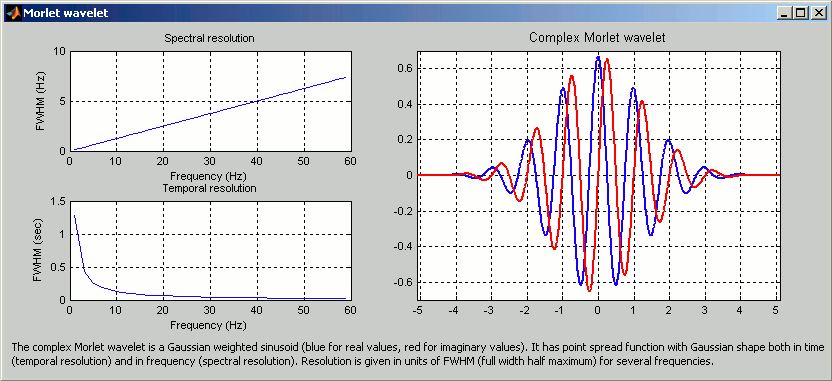
Complex Morlet wavelets are very popular in EEG/MEG data analysis for time-frequency decomposition. They have the shape of a sinusoid, weighted by a Gaussian kernel, and they can therefore capture local oscillatory components in the time series. An example of this wavelet is show below, where the blue and red curves represent the real and imaginary part, respectively.
Contrary to the standard short-time Fourier transform, wavelets have variable resolution in time and frequency. When designing the wavelet, we basically decide a trade off between temporal and spectral resolution.
To design the wavelet, we first need to choose a central frequency, ie the frequency where we will define the mother wavelet. All other wavelets will be scaled and shifted versions of the mother wavelet. Unless interested in designing the wavelet at a particular frequency band, the default 1Hz should be fine.
Then, the desirable time resolution for the central frequency should be defined. For example, we may wish to have a temporal resolution of 3 seconds at frequency 1 Hz (default parameters). These two parameters, uniquely define the temporal and spectral resolution of the wavelet for all other frequencies, as shown in the plots below.
Resolution is given in units of Full Width Half Maximum of the Gaussian kernel, both in time and frequency. The relevant plots are given below.
Edge effects
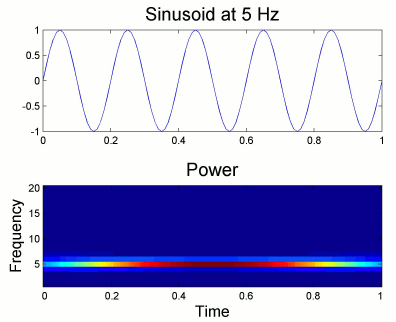
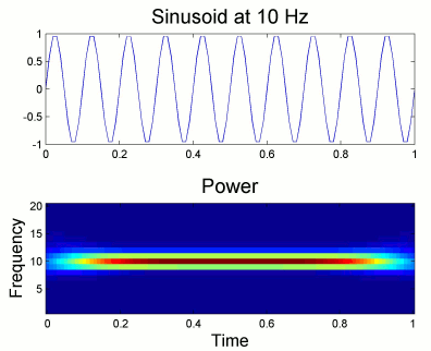
Users should pay attention to edge effects when applying wavelet analysis. Wavelet coefficients are computed by convolving the wavelet kernel with the time series. Similarly to any convolution of signals, there is zero padding at the edges of the time series and therefore the wavelet coefficients are weaker at the begining and end of the timeseries.
From the figure above, which designs the Morlet wavelet, we can see that the default wavelet (central frequency 1Hz, FWHM=3sec) has temporal resolution 0.25sec at 5Hz and 0.1sec at 10Hz. In such case, the edge effects are roughly half these times: 125ms in 5Hz and 50ms in 10Hz. Examples of such edge effects are given in the figures below.
Time-frequency decomposition of MEG Recordings
We are going first to compute the time-frequency decomposition for the two averaged recordings we have in the protocol. Drag'n'drop the two ERF files from Right and Left in Process1. Select "Recordings".
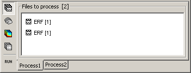
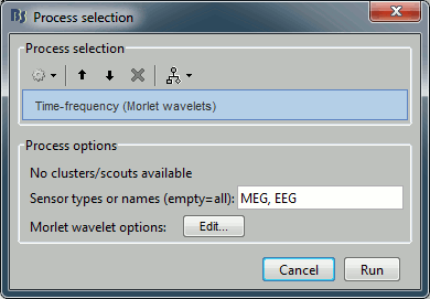
Click on Run. Select the process: Frequency > Time-frequency (Morlet wavelets).
- The only generic option you have access to in this window is the selection of the sensors on which you want to apply the process. You can use this box to select a mixed list of channel types (ex: "MEG") or channel names (ex: "MRT16").
- For now, you can just leave the default "MEG, EEG". There is no EEG channel but it doesn't matter, the extra information is just ignored.
Click on the "Edit" button to get access to the options specific to the time-frequency decomposition process.
Time-frequency option window. You may:
- define bands in time and frequency or analyze the data in all points,
- configure the time and frequency resolution of the wavelets,
- define the output type (complex coefficients or squared coefficients / power).
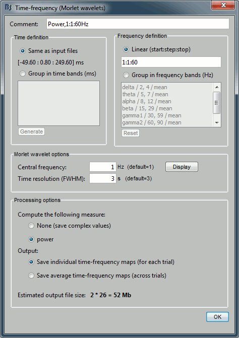
Description of the options
Comment: String that will be displayed in the database explorer to represent the output file.
Time definition:
- This panel describes the time points for which you will get a value at the end of the computation.
Same as input file: If you select this option, you would get the time-frequency decomposition (TF) for each of the time samples in the input file (here: 375 samples between -50ms to 250ms)
Group in time bands: This option adds another step of computation:
- It first computes the TF for each of the time points in the initial file, exactly like with the "same as input file" option
- Then for each time band: it groups the corresponding time points by averaging the power of their TF values.
- Definition of the time bands: two methods
- Enter your own time bands in the text area, one line per time band, with following format: "name : start_time, stop_time"
- Click on the "Generate" button to create automatically a list of time bands with the same length. You will be asked the maximal length of each time band.
Frequency definition:
- This panel describes the frequencies for which the power will be estimated at each time instant.
Linear: You can specify the frequencies with any Matlab syntax start:step:stop. The default is "1:1:30", which produces 60 values [1, 2, 3, 4, ..., 59, 60]
Group in frequency bands: As for the time definition, this option leads to a two-step process:
- It computes the TF for several values in the frequency band (see below ho to define a frequency band)
- Then for each frequency band: it averages the power of all the frequencies in the band, so that you get only one value for each frequency band (and for each time point and each sensor).
- Definition of the frequency bands:
One line per frequency band, with the format "name / frequency definition / function"
- The name can be any string you want
- The frequency definition is a Matlab expression evaluated with an eval() call. If the frequency definition contains only two values, Brainstorm adds two extra values in the middle so that the final averaged value is a bit more robust.
- Examples of valid Matlab expressions:
- "2,4": evaluates to [2,4], and as there are only two values, it uses the frequency vector [2, 2.66, 3.33, 4] instead
- "2, 2.5, 3, 3.5, 4": evaluates to [2 2.5 3 3.5 4]
- "2:4": evalues to [2 3 4]
- "2:0.1:4": evaluates to a vector of 21 values [2 2.1 2.2 2.3 .... 3.8 3.9 4]
- Click on the "Reset" button to go back to the default settings.
Morlet wavelet options:
- Central frequency: frequency where the mother wavelet is designed. All other wavelets will be shifted and scaled versions of the mother wavelet
- Time resolution (FWHM): desirable temporal resolution of the wavelet at the central frequency (in units of Full Width Half Maximum). Click 'display' to see the resolution of the wavelet in other frequencies
- See the first section of this tutorial for a description of those parameters.
Processing options:
Compute the following measure:
- The TF returns the wavelet coefficients for each frequency/time/sensor, which are complex values. Typically, what you want to display is the power of the coefficients, which is the square of the amplitude: abs(TF).^2. You can choose if you want to apply this transformation or not.
Power: Applies the "power" transformation right after the computation. This causes a loss of the phase information.
None: Save the TF coefficients as they are computed. This can be useful if you plan to use those decompositions for other purposes that require the phase, but the files are going to be twice as big.
- If you select "None" here, the power will be computed on the fly for the various displays.
- Some combinations of options may disable this choice. Example: if you ask for time bands or frequency bands, the program will have to compute the power before averaging the values; so in those cases the "None" option is disabled.
Output:
Save individual TF maps: This option stops the computation here, and saves in the database one time-frequency file for each input file.
- Be very careful using this option because if you have hundreds of trials, it will fill your hard drive very quickly.
- One full TF file in this case contains [nSensors x nTime x nFreq] = 3.397.500 values = 25 Mb.
- You can however limit the amount of data produced by using time and/or frequency bands. For 15 time bands and 6 frequency bands, the size of each file drops to: 110 Kb.
Save average TF maps: This option is available only when there are more than one input files (number of files you dropped in the Processes tab).
- Instead of saving the TF for each file separately, it automatically computes the average of the power of all the TF.
- This is a good choice if you do not plan to use independently all the TF files, because it saves a lot of time and disk space.
Computation
Back to our evoked fields. Let's select the following options:
- Time: Same as input
- Frequency: Linear 1:1:60
- Morlet wavelet: 1Hz / 3s
- Output: Power / Individual TF maps (we want one map for the left, and one for the right)
Start the computation:
- Click on "Ok"
- Back to the Pipeline editor, click on "Run".
- After a while, two new files will appear in the tree, representing the TF for the two averaged recordings of the two conditions.
Display time-frequency maps
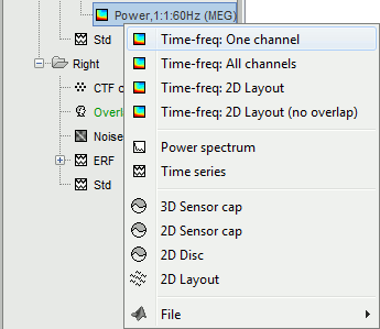
Right-click on the TF file of the Left condition to see what are the possible display options
Time-freq: One channel
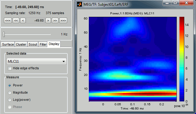
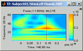
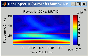
- This is the default view for the TF decompositions of full recordings, ie. what would be displayed if you double-click on this file. It shows for one sensor (or one cluster/scout/source) the power of each frequency at each time.
- When you load time-frequency related files, the "Display" tab automatically appears in the main Brainstorm window to offer some options for the displays, together with the "current frequency" slider.
Current frequency: Slider that shows the current frequency selected in ALL the figures.
Exactly as the time is Brainstorm, the frequency selection/display is centralized and managed by one control only for all the figures. As a consequence, it is impossible to display TF files with different frequency definitions at the same time. This can be perceived as an annoying limitation, but it allows all the simultaneous displays to be consistent at anytime, and make the interface much more intuitive to manipulate, with lower risks of mistakes in the interpretation of the different figures.
Display tab
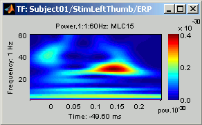
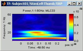
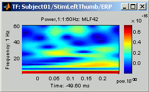
List of sensors: This drop-down list shows the current entry displayed in the selected figure. In this case, it is by default the MEG sensor "MLC11". Try to change it, it will update the display of the figure, showing the frequency power for another sensor.
This selection is relative only to the selected figure, and gets updated when you selected another TF figure.
 -
- 
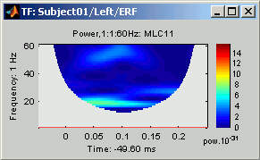
Hide edge effects: When this option is selected, the time-frequency coefficients that could not be properly estimated because of a lack of time samples are hidden. It allows you to see only the information that is really reliable in the selected figure. In this example, you can see that it masks a large portion of the window: 375 time samples are not enough to perform a correct time-frequency decomposition. Try to work on larger time windows when using those tools.
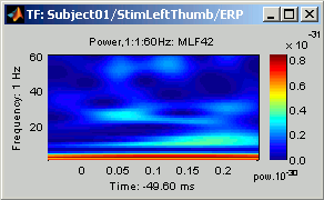
Measure: The selection reflects the type of measure that is currently represented in the selected figure. The entries that are enabled depend on the type of data that is saved in the file. In this case, we saved directly the power of the wavelet coefficients in the file, we discarded the angle/phase information, hence the "phase" option is disabled. If we name "power" the values that are saved in the file in the database, the other options would perform the following operations:
Power: Shows the power values unchanged - (left figure)
Magnitude: Shows sqrt(power) - (right figure)
Log: Shows 10 * log10(power)
 -
- 
Mouse and keyboard
Left-click: Selection of current time and frequency.
- If you click anywhere on a TF figure, it will move the current time/frequency cursor to the clicked point, update the time and the frequency sliders in the Brainstorm window, and also update all other visualization figures.
- If you change the current time or the current frequency with the sliders or with another figure, you would observe that the time/frequency cursor position is updated.
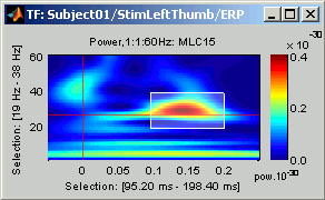
Left-click + move: Select a time/frequency range.
Hold the left mouse button and move the mouse to mark a selection in both time and frequency. The legends of the X and Y axis are updated to display the selected time and frequency ranges selected.
- This selection is used by some functions accessible in the figure's popup menu.
Zoom:
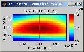
Mouse wheel: Zoom/unzoom in time, centered on the current time cursor.
Control + mouse wheel: Zoom/unzoom in frequencies, centered on the current frequency cursor.
Right-click + move, or Control + left-click + move: Move in the zoomed image.
Double-click: Restore initial view.
Colormap:
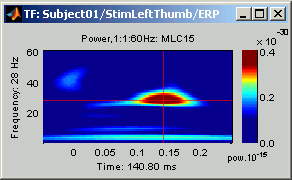
- As explained in the previous tutorials, you can change the colormap by left-clicking on the colorbar on the right of the figure, holding the button, and then by moving the mouse.
- Up/down: Changes the brightness of the colormap.
- Left/Right: Changes the contrast.
This has the same effect than changing the brightness/contrast using the popup menu.
 -
- 
Popup menu: Right-click on the figure.
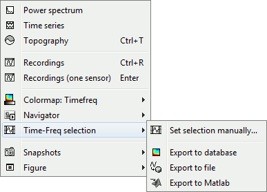
All the menus have been described in the ?tutorial #4 "Exploring the recordings", except for the "Time-frequency selection menu":
(You can see this full menu only if there is a selection defined in the figure)Set selection manually: Does the same thing as drawing a time/freq selection square on a figure, but by typing the values for time and frequency manually.
Export to database: Save the selection for the displayed sensor in a new TF file in the database. However, it is necessary to keep the same time definition for this new file because as it has to stay compatible with the other files it is linked with (here: the recordings file). So in this case, only the selected frequencies are saved, but the time selection is ignored, all the time points are saved.
Remember that only one sensor is exported using this menu, all the others are ignored.Export to file: Same as "Export to database", but the saved file is not registered in the database. The user has to select where to save the file. Unlike the previous menu, only the selected times AND selected frequencies are exported.
Export to Matlab: Same as "Export to file", but the output structure is sent to a variable in the Matlab base workspace instead of being saved to a file.
Keyboard shortcuts:
Left and right arrows: Change the current time
Page-up and page-down: Also change the current time, but faster (10 time samples instead of one)
Up and down arrows: Change the the sensor displayed in this figure (same as using the drop-list in the Display tab)
Control + up and down arrows: Change the current frequency
Enter: View the original time series for this sensor.
Control + R: View the original MEG recordings (this shortcut and the following are visible in the popup menu)
Control + T: View the time-frequency 2D topography (explained in the next sections)
Control + I: Save as image
Control + D: Dock figure in the Matlab environment.
Time-freq: Multiple channels
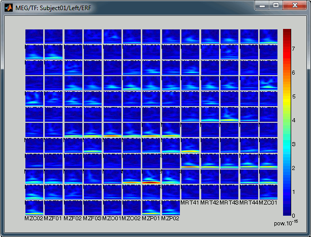
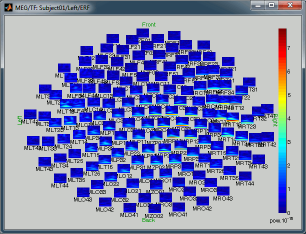
Three menus display the same information (the TF maps of all the channels) with different spatial organizations.
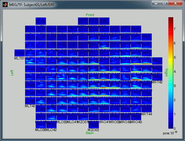
Time-freq: All channels: All the maps are displayed one after the other, in the order they are saved in the file.
Time-freq: 2D Layout: Similarly to the "2D Layout" for the recordings, it shows each the position of each TF map where the sensor is located on a flattened 2D map.
Time-freq: 2D Layout (no overlap): Similar to the "2D Layout", but reorganizing the positions of the small images so that they do not overlap. Overlapping in the "2D Layout" views is not a problem with this old CTF system (151 sensors); it gets much worse with the newer CTF systems (275 sensors), or the Elekta-Neuromag systems (102 chips with 3 sensors at each position). This display is a good intermediate between seeing all the information, and having it spatially organized.
What to do with these figures:
- Maximize the window to be able to see something
Click: clicking on any small TF image opens a new figure to display only the selected sensor
Shift + click: Same, but opens the original recordings time series of the sensor instead of the TF
Mouse wheel: Zoom / unzoom
Left+right mouse click + move: Move in a zoomed figure.
Power spectrum and time series
Those two menus generate similar figures: they represent as a line the evolution of each sensor for one parameter (time or frequency) when the other parameter is fixed.
- Power spectrum: For the given time, show the evolution of all the sensors across the frequencies
- Time series: For the given frequency, show the evolution of all the sensors in time
Open at the same time three figures for the Left/ERF file:
- Time-freq: One channel
- Power spectrum
- Time series.
Then navigate in time and frequencies, and observe how each figure gets updated at each change.
2D topography
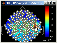
Right-click on the TF file in condition Left and select successively the first three topography menus. All those three windows represent the same information, in a slightly different way: a spatial map of the power of the current frequency, for all the sensors at the current time.
- 3D Sensor cap
- 2D Sensor cap
- 2D Disc
Try to move the time and frequency sliders and see what happens. You can open at the same time a "Time-freq: One channel" view, to keep track easily of the current time and frequency.
Keyboard shortcuts:
Left and right arrows: Change the current time
Page-up and page-down: Also change the current time, but faster (10 time samples instead of one)
Up and down arrows: Change the current frequency
Control + E: Display the sensors markers
Control + E again: Display the sensors names
Shift + Click on a sensor: Displays the time-frequency decomposition for that specific sensors.
2D Layout
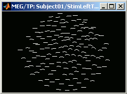
- The last display mode available for those TF decomposition of recordings is this "2D Layout" topography menu. Right-click on the TF file for the Left condition and select "2D Layout".
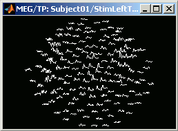
This represents spatially the power of the current frequency for all the sensors and all the time points. Try to move the current frequency slider to see how the display changes when increasing the frequency. It is a good example to show that the time resolution increase with the frequency. Below: the "2D Layout" displays for f=8Hz and f=60Hz.
- Useful operations for this window:
Mouse wheel: Zoom / unzoom
Left+right click + move: (or middle click+move) Move into the zoomed window
Shift+mouse wheel: Increase/decrease the sharpness of the time series
Control + mouse wheel: Increase/decrease the length of the time window displayed around the current time.
Click on a line: Select a sensor
Right click + move: Select a group of sensors
Shift + click on a line: Display the time-frequency decomposition for the selected sensor
Right-click: Display popup menu. More options in the "2D Layout options" sub-menu.
Control + E: Display the channels names
All the other shortcuts and the popup menu are already described in ?tutorial #4 "Exploring the recordings".
Contents of the "timefreq" files
Right click one of the TF files, and select the menu File > View file contents, to have a look to what is the actual contents of those structures.
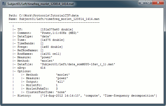
TF: [nSensors x nTime x nFrequency] matrix containing all the values of the time-frequency decomposition (complex wavelet coefficients, or power of amplitudes)
- nSensors: Number of sensors for which the TF has been estimated
- nTime:
If there are time bands defined, nTime = size(TimeBands,1) = number of time bands
- If there are no time bands (linear time sampling): nTime = length(Time)
- nFrequency:
- If there are frequency bands defined, nFrequency = size(Freqs,1) = number of frequency bands
- If there are no frequency bands (linear frequency sampling): nFrequency = length(Freqs
Comment: String displayed in the database explorer to represent the file.
DataType: Explains from what kind of data this file was computed. Possible values are: 'data', 'results', 'cluster', 'scout'
Time: Time vector used to estimate this file.
TimeBands: Description of the time bands. Cell array {nTimeBands x 3}, where each line represents a time band {'band_name', time_start, time_stop}
Freqs:
- If frequecy bands: Cell array {nFreqBands x 3}, where each line represents a frequency band {'band_name', freq_start, freq_stop}
- In linear frequency sampling: vector containing all the frequencies
RowNames: Cell array of strings that describes each row of the TF matrix. In this specific case, it would be the list of all the MEG sensor names. But it could also be a list of names of scouts or clusters.
Measure: Contains the name of the function that was applied right after the computation of the wavelet coefficients. So it represents the type of data contained in the TF matrix. Possible values:
- Empty matrix: No measure applied, TF contains the complex wavelet coefficients.
- 'Power': TF contains the power for each frequency, ie. the square of the amplitude: abs(coefficients).^2
DataFile: Initial file from which this file was computed. In the database explorer, the TF file will be shown as a child of this DataFile file.
ChannelFlag: Good/bad channel vector of the recordings file at the time the TF file was computed
nAvg: Number of trials that were averaged to obtain this file (copied from the recordings file at computation)
History: List of operations performed on this file (better visualized with popup menu File > View file history)
Options: Options that were selected in the time-frequency options window.
Time and frequency bands
Frequency bands
Drag'n'drop the averaged file Left / ERF in the Process tab, click on Run, select Analyze > Time-frequency decomposition. Click on Ok.
- Just change the frequency definition: select "Group in frequency bands", leave the default frequency bands, and click on Ok.
Right-click on the file you've just computed "Power,FreqBands" > Time-frequency maps.
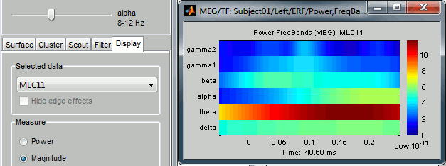
- You can notice that now the frequency selection is discreet, both in the figure and in the frequency slider, it is not possible to select a frequency in between. At each time and for each sensor, there are now just 6 values, one per frequency band.
- Now if you try to open at the same time the first TF that you have computed "Power,1:1:60Hz", you would get an error message: This frequency definition is not compatible for display with the linear [1...60] scale.
- Display the other possible views (All sensors, 2D Sensor Cap, 2D Layout), and change the current time and the current frequency in different ways (sliders, keyboard, clicks on figures). Play with the open figures until you are completely comfortable with those representations.
Time bands
Compute TF again for file Left / ERF, but this time select the option "Group in time bands" (with "linear" frequency definition). To generate a list of regular time intervals, click on "Generate" and enter "30" ms as the duration of each time band.
- You get 11 time bands: t-2 and t-1 before 0ms, and t1 to t9 after 0ms. Click on Ok to start the computation.
Right-click on this new file "Power,1:1:60Hz" > Time-frequency maps.
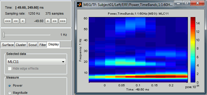
- Observe that the behavior is not the same as with the frequency bands: it is still possible to select a specific time in a time band (using the slider or clicking on the figure). This is because the time definition in the interface is still based on the ERF averaged file time definition, which is "continuous". Only 11 values in time are computed, and when requesting values a specific time point, the interface gets the values associated with the time band that time point belongs to.
- As a consequence, it is possible to open at the same time the first TF file that you have computed: "Power,1:1:60Hz". You would not get an error message like with the frequencies mismatching.
- Display also other types of figures (All sensors, 2D topographies), change current time and frequency several times in serveral ways (sliders, keyboard, clicks on figures).
Time bands and frequency bands
Just for curiosity, compute a file with both time and frequency bands.
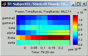
TF: Clusters time series
- Create two clusters "c1" and "c2" for the Left condition.
Display a time series view for the Left / ERF average:
- Select a few sensors, and click on the "New sel" button in the "Cluster" tab.
- Press "Escape" to unselect all the selected sensors.
- Select another group of sensors, and click on the "New sel" button again.
Drag'n'drop the Left / ERF file in the Processes list. Click on run.
Select the process "Analysis > Time-frequency decomposition".
As some clusters are now available, you can have access to them in this interface.
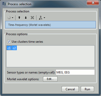
- Check the option "Use clusters time series", and select them both.
- The TF decomposition will be done for all the channels, but only on the averaged time series for each cluster.
Click on run. A new option is displayed in the options window, "Cluster function"

- The selection of the "cluster function" is done in the "Cluster" tab.
Before: The selected function (in this case: mean), is applied to get only one time serie for each cluster, and the TF is computed only for those processed time series. Faster, but may cause a loss of information, if the phase is slightly different for each sensor.
After: The TF is computed for all the sensors, and then then the selected function (mean) is applied to the power of those TF to get only one TF decomposition for each cluster. Slower, but more representative of the power of each frequency.
- When the selected function is "All", this option doesn't appear because there is no function applied, it computes the TF for all the sensors.
- Do not change any TF option, click on OK.
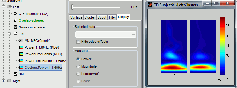
A new file "Clusters,Power,1:1:60Hz" appears in the database. The size of TF matrix in this file is [nClusters x nTimes x nFrequencies] = [2 x 375 x 60]. Double-click on it. The list in the "Time-freq" tab only contains two items: c1 and c2.
TF: Cortical sources
- How to display the TF decompositions for the source time series?
- It is possible to estimate the TF for each source of the brain, but it would be unrealistic to save this information to a file. The size of the TF matrix would be [nVertices x nTimes x nFrequencies] = [15010 x 375 x 60] complex-double = 5.2 Gb!
- We need then to simplify this problem. Two methods: compute the TF only for a few scouts (next section), or use the linear property of the TF decomposition.
As both the source reconstruction process (ImagingKernel * recordings) and the TF are linear operators, it is possible to exchange them:
TF(Inverse(Recordings)) = Inverse(TF(Recordings))
=> Power(TF(Inverse(Recordings))) = Power(Inverse(TF(Recordings)))So the solution is to estimate the TF of the recordings, and then multiply it on the fly by the ImagingKernel only for the required sources and/or frequency and/or time instant. This is done in a completely transparent way from the user point a view.
- Start the computation of the TF for a source file:
Drag'n'drop the source file computed for the Left / ERF file in Process1.
- Select the "Process sources" button.
- Click on Run. Select "Time-frequency decomposition" and click on Ok.
Note that almost all the options are disabled. This is because the Power transformation is non-linear: we need to keep the complex Morlet wavelet coefficients. Those complex values will be first multiplied by the ImagingKernel matrix; the power is computed after, for display only.
- As a consequence, it is impossible to compute time or frequency bands now, because they are averages of the power values.
Click on Ok. A new file appears in the database explorer, as a child of the source file. Right-click on it, try all the visualization menus.
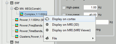
If you understood well how to use the visualization of both the sources and the time-frequency maps, the manipulation of those figures should be rather intuitive. Change several times the current time and the current frequency in different ways.
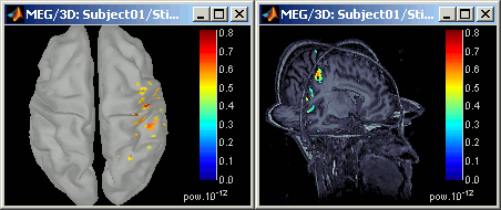
Shift + click on the cortex surface: This is a useful shortcut that you should remember. It displays the TF decomposition of the selected source.
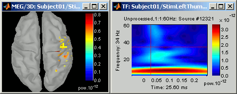
TF: Scouts time series
It is interesting to display the TF for a single source, but it is hard to extract synthetic information that can be analyzied statistically or compared between subjects this way. A better option is to define cortical regions of interest (scouts, see ?tutorial #8), and compute the TF for the average time serie of these scouts.
- Create scouts:
Right-click on the TF file for the ERF source file of condition Left. Select "Display on cortex".
- Change current time and frequency so that you can observe the main response in the somato-sensory cortex (eg. t = 46.40ms, f = 45Hz).
In the "Scout" tab, load the two scouts LeftSS and RightSS that you created in tutorial #8 (or create two scouts).
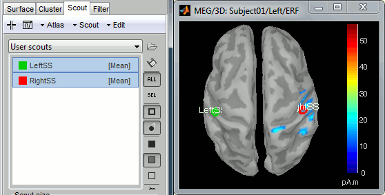
- Compute the TF decomposition for these scouts:
Drag'n'drop the sources file (MN: MEG(Constr)) into Process1.
- Select the "Process sources" button.
Click on Run. Select "Analyze > Time-frequency decomposition".
As some scouts are defined, you will see this new box:
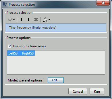
- Select "Use scouts time series", and select both scouts in list. Click on Ok.
- This time, most of the options are available again. We are going to compute the full TF matrix at once for the two scouts, so we can compute the power right away, together with time and/or frequency bands.
- Do not change any option and click on Ok. A new file appears in the tree, as a child of the sources file: "Scouts,Power,1:1:60Hz".
- To compute the TF of each scout, the operations are the following:
- Get time series for each source in the scout
If the scout function is applied before the TF:
- Apply the "scout function", that combines the different sourcesto get only one time serie for each scout.
- Compute the power of the TF for each scout.
If the scout function is applied after the TF:
- Compute the power of the TF for each source
- Apply the "scout function", that combines the different sources TF to get one TF only for each scout.
- The selection of the "scout function" is done in the "Scout" tab.
Right-click on this file and try the two visualization menus available.

Processing time-frequency files
Time-frequency files, once computed, can be processed with Process1 and Process2, exactly as recordings or sources file, as introduced in ?Tutorial #9.
- Only the TF of sensors, clusters and scouts can be processed this way.
- The TF of full source files, as explained above, are saved in the database in an incomplete form, that requires a few more on-the-fly computation steps. The processing engine requires an access to the full TF matrix, which is usually too big to be handled in Matlab for those TF/sources files.
- If you need to average or do some group-analysis on time-frequency data at the source level, the problem has to be simplified a few steps before: for instance by doing your analysis only on a few scouts instead of the full cortex.
Drag'n'drop the TF files in the Processes panel, select the "Time-freq" button, click on Run, and select a process.
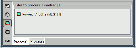
Warning: Those features are still experimental, they might not work properly. Note also that it is impossible to display yet the results of the t-tests on TF files.
Z-SCORE
Next
This is the last tutorial for Brainstorm introduction. You had an overview of most of the software features. Now you can go back to the main Tutorials page, and read tutorials that are closer to your area of interest.

