|
Size: 34466
Comment:
|
Size: 23011
Comment:
|
| Deletions are marked like this. | Additions are marked like this. |
| Line 2: | Line 2: |
| ''Authors: Francois Tadel, Elizabeth Bock.'' The aim of this tutorial is to reproduce the analysis and results o The aim of this tutorial is to provide high-quality recordings of a simple auditory stimulation and illustrate the best analysis paths possible with Brainstorm and FieldTrip. This page presents the workflow in the Brainstorm environment, the equivalent documentation for the FieldTrip environment will be available on the [[http://fieldtrip.fcdonders.nl/|FieldTrip website]]. Note that the operations used here are not detailed, the goal of this tutorial is not to teach Brainstorm to a new inexperienced user. For in depth explanations of the interface and the theory, please refer to the introduction tutorials. |
''Authors: Francois Tadel, Elizabeth Bock. '' The aim of this tutorial is to reproduce in the Brainstorm environment the analysis described in the SPM tutorial "[[ftp://ftp.mrc-cbu.cam.ac.uk/personal/rik.henson/wakemandg_hensonrn/Publications/SPM12_manual_chapter.pdf|Multimodal, Multisubject data fusion]]". The data processed here consists in simulateneous MEG/EEG recordings of 16 (19) subjects performing simple visual task on a large number of famous, unfamiliar and scrambled faces. The analysis is split in two tutorial pages: the present tutorial describes the detailed analysis of one single subject and another one that the describes the batch processing and [[Tutorials/VisualGroup|group analysis of the 16 subjects]]. Note that the operations used here are not detailed, the goal of this tutorial is not to teach Brainstorm to a new inexperienced user. For in depth explanations of the interface and the theory, please refer to the introduction tutorials. |
| Line 12: | Line 12: |
| == License == These data are provided freely for research purposes only (as part of their Award of the BioMag2010 Data Competition). If you wish to publish any of these data, please acknowledge Daniel Wakeman and Richard Henson. The best single reference is: Wakeman DG, Henson RN, [[http://www.nature.com/articles/sdata20151|A multi-subject, multi-modal human neuroimaging dataset]], Scientific Data (2015) Any questions, please contact: rik.henson@mrc-cbu.cam.ac.uk == Presentation of the experiment == ==== Experiment ==== * 19 subjects * 6 runs (sessions) of approximately 10mins for each subject * Presentation of series of images: familiar faces, unfamiliar faces, phase-scrambled faces * The subject has to judge the left-right symmetry of each stimulus * Total of nearly 300 trials in total for each of the 3 conditions ==== MEG acquisition ==== * Acquisition at 1100Hz with an Elekta-Neuromag VectorView system (simultaneous MEG+EEG). * Recorded channels (404): * 102 magnetometers * 204 planar gradiometers * 70 EEG electrodes recorded with a nose reference. * MEG data have been "cleaned" using Signal-Space Separation as implemented in MaxFilter 2.1. * A Polhemus digitizer was used to digitise three fiducial points and a large number of other points across the scalp, which can be used to coregister the M/EEG data with the structural MRI image. * The distribution contains 3 sub-directories of empty-room recordings of 3-5mins acquired at roughly the same time of year (spring 2009) as the 19 subjects. The sub-directory names are Year (first 2 digits), Month (second 2 digits) and Day (third 2 digits). Inside each are 2 raw *.fif files: one for which basic SSS has been applied by maxfilter in a similar manner to the subject data above, and one (*-noSSS.fif) for which SSS has not been applied (though the data have been passed through maxfilter just to convert to float format). ==== Subject anatomy ==== * MRI data acquired on a 3T Siemens TIM Trio: 1x1x1mm T1-weighted structural MRI * Processed with FreeSurfer 5.3 |
|
| Line 13: | Line 40: |
| * '''Requirements''': You have already followed all the basic tutorials and you have a working copy of Brainstorm installed on your computer. * Go to the [[http://neuroimage.usc.edu/brainstorm3_register/download.php|Download]] page of this website, and download the file: '''sample_auditory.zip ''' * Unzip it in a folder that is not in any of the Brainstorm folders (program folder or database folder). This is really important that you always keep your original data files in a separate folder: the program folder can be deleted when updating the software, and the contents of the database folder is supposed to be manipulated only by the program itself. * Start Brainstorm (Matlab scripts or stand-alone version) * Select the menu File > Create new protocol. Name it "'''TutorialAuditory'''" and select the options: |
* The data is hosted on this FTP site (use an FTP client such as FileZilla, not your web browser): <<BR>>ftp://ftp.mrc-cbu.cam.ac.uk/personal/rik.henson/wakemandg_hensonrn/ * Alternative to discuss: use the original 19 subjects from the openfmri website: <<BR>>https://openfmri.org/dataset/ds000117/ * Download only the following folders (about 75Gb): * '''EmptyRoom''': MEG empty room measurements. * '''SubXX/MEEG/*_sss.fif''': MEG and EEG recordings in FIF format, corrected with SSS. * '''SubXX/MEEG/Trials''': Trials definition files. * '''Publications''': Reference publications related with this dataset. * '''README.TXT''': License and dataset description. * The FreeSurfer segmentations of the T1 images are not part of this package. You can either process them by yourself, or download the result of the segmentation from the Brainstorm website. <<BR>>Go to the [[http://neuroimage.usc.edu/bst/download.php|Download]] page, and download the file: '''sample_group_anat.zip'''<<BR>>Unzip this file in the same folder where you downloaded all the datasets. * Reminder: Do not put the downloaded files in the Brainstorm folders (program or database folders). * Start Brainstorm (Matlab scripts or stand-alone version). For help, see the [[Installation]] page. * Select the menu File > Create new protocol. Name it "'''TutorialVisual'''" and select the options: |
| Line 24: | Line 58: |
| * Right-click on the TutorialAuditory folder > New subject > '''Subject01''' | * Right-click on the TutorialAuditory folder > New subject > '''Sub001''' |
| Line 28: | Line 62: |
| * Select the folder: '''sample_auditory/anatomy''' | * Select the folder: '''Anatomy/Sub001''' (from sample_group_anat.zip) |
| Line 30: | Line 64: |
| * Set the 6 required fiducial points (indicated in MRI coordinates): * NAS: x=127, y=213, z=139 * LPA: x=52, y=113, z=96 * RPA: x=202, y=113, z=91 * AC: x=127, y=119, z=149 * PC: x=128, y=93, z=141 * IH: x=131, y=114, z=206 (anywhere on the midsagittal plane) * At the end of the process, make sure that the file "cortex_15000V" is selected (downsampled pial surface, that will be used for the source estimation). If it is not, double-click on it to select it as the default cortex surface. {{attachment:anatomy.gif||height="264",width="335"}} |
* The two sets of fiducials we usually have to define interactively are here automatically set. * '''NAS/LPA/RPA''': The file Anatomy/Sub01/fiducials.m contains the definition of the nasion, left and right ears. The anatomical points used by the authors are the same as the ones we recommend in the Brainstorm [[CoordinateSystems|coordinates systems page]]. * '''AC/PC/IH''': Automatically identified using the SPM affine registration with an MNI template. * If you want to double-check that all these points were correctly marked after importing the anatomy, right-click on the MRI > Edit MRI. * At the end of the process, make sure that the file "cortex_15000V" is selected (downsampled pial surface, that will be used for the source estimation). If it is not, double-click on it to select it as the default cortex surface. Do not worry about the big holes in the head surface, parts of MRI have been remove voluntarily for anonymization purposes.<<BR>><<BR>> {{attachment:anatomy_import.gif||height="384",width="613"}} * All the anatomical atlases [[Tutorials/LabelFreeSurfer|generated by FreeSurfer]] were automatically imported: the surface-based cortical atlases and the atlas of sub-cortical regions (ASEG). <<BR>><<BR>> {{attachment:anatomy_atlas.gif||height="211",width="550"}} |
| Line 43: | Line 76: |
| * Right-click on the subject folder > Review raw file * Select the file format: "'''MEG/EEG: CTF (*.ds...)'''" * Select all the .ds folders in: '''sample_auditory/data''' {{attachment:raw1.gif||height="156",width="423"}} * Refine registration now? '''YES'''<<BR>><<BR>> {{attachment:raw2.gif||height="224",width="353"}} === Multiple runs and head position === * The two AEF runs 01 and 02 were acquired successively, the position of the subject's head in the MEG helmet was estimated twice, once at the beginning of each run. The subject might have moved between the two runs. To evaluate visually the displacement between the two runs, select at the same time all the channel files you want to compare (the ones for run 01 and 02), right-click > Display sensors > MEG.<<BR>><<BR>> {{attachment:raw3.gif||height="220",width="441"}} * Typically, we would like to group the trials coming from multiple runs by experimental conditions. However, because of the subject's movements between runs, it's not possible to directly compare the sensor values between runs because they probably do not capture the brain activity coming from the same regions of the brain. * You have three options if you consider grouping information from multiple runs: * '''Method 1''': Process all the runs separately and average between runs at the source level: The more accurate option, but requires a lot more work, computation time and storage. * '''Method 2''': Ignore movements between runs: This can be acceptable for commodity if the displacements are really minimal, less accurate but much faster to process and easier to manipulate. * '''Method 3''': Co-register properly the runs using the process Standardize > Co-register MEG runs: Can be a good option for displacements under 2cm.<<BR>>Warning: This method has not be been fully evaluated on our side, to use at your own risk. Also, it does not work correctly if you have different SSP projectors calculated for multiple runs. * In this tutorial, we will illustrate only method 1: runs are not co-registered. === Epoched vs. continuous === * The CTF MEG system can save two types of files: epoched (.ds) or continuous (_AUX.ds). * Here we have an intermediate storage type: continuous recordings saved in an "epoched" file. The file is saved as small blocks of recordings of a constant time length (1 second in this case). All these time blocks are contiguous, there is no gap between them. * Brainstorm can consider this file either as a continuous or an epoched file. By default it imports the regular .ds folders as epoched, but we can change this manually, to process it as a continuous file. * Double-click on the "Link to raw file" for run 01 to view the MEG recordings. You can navigate in the file by blocks of 1s, and switch between blocks using the "Epoch" box in the Record tab. The events listed are relative to the current epoch.<<BR>><<BR>> {{attachment:raw4.gif||height="206",width="575"}} * Right-click on the "Link to raw file" for run 01 > '''Switch epoched/continuous''' * Double-click on the "Link to raw file" again. Now you can navigate in the file without interruptions. The box "Epoch" is disabled and all the events in the file are displayed at once.<<BR>><<BR>> {{attachment:raw5.gif||height="209",width="576"}} * Repeat this operation twice to convert all the files to a continuous mode. * '''Run 02''' > Switch epoched/continuous * '''Noise''' > Switch epoched/continuous == Stimulation triggers delay == === Evaluation === * Right-click on Run01/Link to raw file > '''Stim '''> Display time series (stimulus channel, UPPT001)<<BR>>Right-click on Run01/Link to raw file > '''ADC V''' > Display time series (audio signal generated, UADC001) * In the Record tab, set the duration of display window to '''0.200s'''.<<BR>>Jump to the third event in the "standard" category. * We can observe that there is a delay of about '''13ms''' between the time where the stimulus trigger is generated by the stimulation computer and the moment where the sound is actually played by the sound card of the stimulation computer ('''delay #1'''). This is matching the documentation of the experiment in the first section of this tutorial. <<BR>><<BR>> {{attachment:stim1.gif||height="282",width="590"}} === Correction === * '''Delay #1''': We can detect the triggers from the analog audio signal (ADC V/UADC001) rather than using the events already detected by the CTF software from the stim channel (Stim/UPPT001). * Drag and drop '''Run01 '''and '''Run02 '''to the Process1 box. * Add __'''twice'''__ the process "'''Events > Detect analog triggers'''".<<BR>>Once with event name="standard_fix" and reference event="standard".<<BR>>Once with event name="deviant_fix" and reference event="deviant".<<BR>>Set the other options as illustrated below:<<BR>><<BR>> {{attachment:stim2.gif}} * Open Run01 (channel ADC V) to evaluate the correction that was performed by this process. If you look at the third trigger in the "standard" category, you can measure a 14.6ms delay between the original event "standard" and the new event "standard_fix".<<BR>><<BR>> {{attachment:stim3.gif||height="151",width="570"}} * Open '''Run01''' to re-organize the event categories: * '''Delete '''the unused event categories: '''standard''', '''deviant'''. * '''Rename '''standard_fix and deviant_fix to '''standard''' and '''deviant'''. * Open '''Run02''' and do the same cleaning operations:<<BR>><<BR>> {{attachment:stim5.gif||height="149",width="502"}} * '''Important note''': We compensated for the jittered delays (delay #1), but not for the other ones (delays #2, #3 and #4). There is still a''' constant 5ms delay''' between the stimulus triggers ("standard" and "deviant") and the time where the sound actually reaches the subject's ears. == Detect and remove artifacts == |
* Right-click on the subject folder > '''Review raw file'''. * Select the file format: "'''MEG/EEG: Neuromag FIFF (*.fif)'''" * Select the '''first''' FIF files in: '''Sub001/MEEG''' <<BR>><<BR>> {{attachment:review_raw.gif||height="181",width="446"}} * Events:''' Ignore'''<<BR>>We will read events for the stimulus channel and define trial definitions later.<<BR>><<BR>> {{attachment:review_ignore.gif||height="186",width="330"}} * Refine registration now? '''NO''' <<BR>>The head points that are available in the FIF files contain all the points that were digitized during the MEG acquisition, including the ones corresponding to the parts of the face that have been removed from the MRI. If we run the fitting algorithm, all the points around the nose will not match any close points on the head surface, leading to a wrong result. We will first remove the face points and then run the registration manually. === Channel classification === A few non-EEG channels are mixed in with the EEG channels, we need to change this before applying any operation on the EEG channels. * Right-click on the channel file > '''Edit channel file'''. Double-click on a cell to edit it. * Change the type of '''EEG062''' to '''EOG '''(electrooculogram). * Change the type of '''EEG063 '''to '''ECG '''(electrocardiogram). * Change the type of '''EEG061''' and '''EEG064''' to '''NOSIG'''. <<BR>><<BR>> {{attachment:channel_edit.gif||height="252",width="561"}} === MRI registration === * Right-click on the channel file > '''Digitized head points > Remove points below nasion'''.<<BR>><<BR>> {{attachment:channel_remove.gif||height="194",width="329"}} * Right-click on the channel file > '''MRI registration > Refine registration'''.<<BR>><<BR>> {{attachment:channel_refine.gif||height="173",width="294"}} * MEG/MRI registration, before (left) and after (right) this automatic registration procedure: <<BR>><<BR>> {{attachment:registration.gif||height="209",width="236"}} {{attachment:registration_final.gif||height="208",width="237"}} * Right-click on the channel file > MRI registration > EEG: Edit...<<BR>>Click on ['''Project electrodes on surface''']<<BR>><<BR>> {{attachment:channel_project.gif||height="207",width="477"}} * Close all the windows (use the [X] button at the top-right corner of the Brainstorm window). === Import event markers === * Right-click on the "Link to raw file" > '''MEG (all) > Display time series'''. * In the Record tab, menu '''File > Read events from channel'''. * Event channels: '''STI101''' * Select '''Value''' <<BR>><<BR>> {{attachment:events_read_channel_STI101.png||height="200",width="300"}} * Three event markers represent each trial type that we will explore in this analysis and need to be merged to one event. * In the Record tab, menu '''Events > Merge groups''' combine the following events to create the labeled groups: * Famous: 5,6,7 * Unfamiliar: 8,9,10 * Scrambled: 11,12,13 <<BR>><<BR>> {{attachment:events_merge.png||height="200",width="300"}} * Because the detection only looks for values, multiple events can be detected in one trial. For example, a value of 7 represents a Famous trial, but during the trial another event occurred as well. The value went from 7 to 4101, for example, and then back to 7. In this case, the 7 would be counted twice. * In the Record tab, menu '''Events > Detect multiple responses''', remove the extra events * Response events: '''Famous''' * Minimum delay between events: '''2200ms''' * Select '''Keep only the first event''' <<BR>><<BR>> {{attachment:events_detect_multiple.png||height="250",width="300"}} * The stimulus presentation to the subject has a delay of 34.5ms, which can be corrected with an offset. * In the Record tab, menu '''Events > Add time offset''' * Event names: '''Famous''' * Time offset: '''34.5ms''' <<BR>><<BR>> {{attachment:events_add_time_offset.png||height="250",width="300"}} * Complete these same steps (merge, detect multiple and add time offset) for types Unfamiliar and Scrambled. == Pre-processing == |
| Line 89: | Line 121: |
| * One of the typical pre-processing steps consist in getting rid of the contamination due to the power lines (50 Hz or 60Hz). Let's start with the spectral evaluation of this file. * Drag '''ALL''' the "Link to raw file" to the Process1 box, or easier, just drag the node "Subject01", it will select recursively all the files in it. * Run the process "'''Frequency > Power spectrum density (Welch)'''": * Time window: '''[All file]''', Window length: '''4s''', Overlap: '''50%''', Sensor types: '''MEG''' * Note that you need at least 8Gb of RAM to run the PSD on the entire file. If you don't or if you get "Out of memory" errors, you can try running the PSD on a shorter time window. * Click on '''[Edit]''' and select option "'''Save individual PSD values''' (for each trial)".<<BR>><<BR>> {{attachment:psd1.gif||height="394",width="615"}} * Double-click on the new PSD files to display them. * Observations for '''Run''''''01''': <<BR>><<BR>> {{attachment:psd_eval01.gif||height="207",width="394"}} * Peaks related with the power lines: '''60Hz, 120Hz, 180Hz '''(240Hz and 300Hz could be observed as well depending on the window length used for the PSD) * The drop after '''600Hz''' corresponds to the low-pass filter applied at the acquisition time. * One channel indicates a higher noise than the others in high frequencies: '''MLO52''' (in red).<<BR>>We will probably mark it as bad later, when reviewing the recordings. * Observations for '''Run02''': <<BR>><<BR>> {{attachment:psd_eval02.gif||height="208",width="394"}} <<BR>> {{attachment:psd_eval02_zoom.gif||height="208",width="595"}} * Same peaks related with the power lines: '''60Hz, 120Hz, 180Hz''' * Same drop after '''600Hz'''. * Same noisy channel: '''MLO52'''. * Additionally, we observe higher level of noise in frequencies in the range of 30Hz to 100Hz on '''many occipital sensors'''. This is probably due to some tension in the neck due to an uncomfortable position. We will see later whether these channels need to be tagged as bad. === Power line contamination === * Put '''ALL''' the "Link to raw file" into the Process1 box (or directly the Subject01 folder) * Run the process: '''Pre-process > Notch filter''' * Select the frequencies: '''60, 120, 180 Hz''' * Sensor types or names: '''MEG''' * The higher harmonics are too high to bother us in this analysis, plus they are not clearly visible in all the recordings. * In output, this process creates new .ds folders in the same folder as the original files, and links the new files to the database.<<BR>><<BR>> {{attachment:psd3.gif}} * Run again the PSD process "'''Frequency > Power spectrum density (Welch)'''" on these new files, with the same parameters, to evaluate the quality of the correction. * Double-click on the new PSD files to open them.<<BR>><<BR>> {{attachment:psd5.gif||height="177",width="416"}} * Zoom in with the mouse wheel to observe what is happening around 60Hz (before / after).<<BR>><<BR>> {{attachment:psd6.gif||height="143",width="453"}} * To avoid the confusion later, delete the links to the original files: Select the folders containing the original unfiltered files and press the Delete key (or right-click > File > Delete).<<BR>><<BR>> {{attachment:psd7.gif||height="184",width="356"}} === Heartbeats and eye blinks === * Select the two AEF runs in the Process1 box. * Select successively the following processes, then click on [Run]: * '''Events > Detect heartbeats:''' Select channel '''ECG''', check "All file", event name "cardiac". * '''Events > Detect eye blinks:''' Select channel '''VEOG''', check "All file", event name "blink". * '''Events > Remove simultaneous''': Remove "'''cardiac'''", too close to "'''blink'''", delay '''250ms'''. * '''Compute SSP: Heartbeats''': Event name "cardiac", sensors="MEG", '''do not use existing SSP'''. * '''Compute SSP: Eye blinks''': Event name "blink", sensors="MEG", '''do not use existing SSP'''.<<BR>><<BR>> {{attachment:ssp_pipeline.gif||height="359",width="527"}} * Double-click on '''Run01 '''to open the MEG.<<BR>>You can change the color of events "standard" and "deviant" to make the figure more readable. * Review the '''EOG '''and '''ECG '''channels and make sure the events detected make sense.<<BR>><<BR>> {{attachment:events.gif||height="369",width="557"}} * In the Record tab, menu SSP > '''Select active projectors'''. * Blink: The first component is selected and looks good. * Cardiac: The category is disabled because no component has a value superior to 12%. * Select the first component of the cardiac category and display its topography. * It looks exactly like a cardiac topography, keep it selected and click on [Save].<<BR>><<BR>> {{attachment:ssp_result.gif||height="172",width="700"}} * Repeat the same operations for '''Run02''': * Review the events. * Select the first cardiac component. === Bad segments === * At this point, you should review the entire files, by pages of a few seconds scrolling with the F3 key, to identify all the bad channels and the noisy segments of recordings. Do this with the the EOG channel open at the same time to identify saccades or blinks that were not completely corrected with the SSP projectors. As this is a complicated task that requires some expertise, we have prepared a list of bad segments for these datasets. * Open '''Run01'''. In the Record tab, select '''File > Add events from file''': * File name: sample_auditory/data/S01_AEF_20131218_01_notch/'''events_bad_01.mat ''' * File type: Brainstorm (events*.mat) * It adds '''12 bad segments''' to the file. * Open '''Run02'''. In the Record tab, select '''File > Add events from file''': * File name: sample_auditory/data/S01_AEF_20131218_02_notch/'''events_bad_02.mat ''' * File type: Brainstorm (events*.mat) * It adds '''9 bad segments''' and '''16 saccades''' to the file. === Saccades === * Run02 contains a few saccades that generate a large amount of noise in the MEG recordings. They are not identified well by the automatic detection process based on the horizontal EOG. We have marked some of them, you have already loaded these events together with the bad segments. We are going to use again the SSP technique to remove the spatial components associated with these saccades. * Open the MEG recordings for '''Run02''' and select the right-frontal sensors (Record tab > CTF RF). * In the Record tab, menu SSP > Compute SSP: Generic<<BR>>Event name='''saccade''', Time='''[0,500]ms''', Frequency='''[1,15]Hz''', '''Use existing SSP'''<<BR>><<BR>> {{attachment:ssp_saccade_process.gif||height="442",width="329"}} * Example of saccade without correction:<<BR>><<BR>> {{attachment:ssp_saccade_before.gif||height="259",width="711"}} * With the first component of saccade SSP applied: <<BR>><<BR>> {{attachment:ssp_saccade_after.gif||height="283",width="507"}} * This first component removes really well the saccade, keep it selected and click on [Save]. === Bad channels === * During the visual exploration, some channels appeared generally noisier than the others. Example: <<BR>><<BR>> {{attachment:badchannel02.gif||height="200",width="456"}} * Right-click on '''Run01 '''> Good/bad channels > Mark some channels as bad<<BR>> > '''MRT51, MLO52''' * Right-click on '''Run02 '''> Good/bad channels > Mark some channels as bad<<BR>> > '''MRT51, ''''''MLO52, MLO42, MLO43''' |
* Drag and drop the "Link to raw file" in Process1. {{attachment:psd_select.gif||height="106",width="388"}} * Run process "'''Frequency > Power spectrum density (Welch)'''" with the options illustrated below. <<BR>><<BR>> {{attachment:psd_process.gif||height="321",width="543"}} * Right-click on the PSD file > Power spectrum. <<BR>><<BR>> {{attachment:psd_plot.gif||height="315",width="546"}} * Observations: * Three groups of sensors, from top to bottom: EEG, MEG gradiometers, MEG magnetometers. * Power lines: '''50 '''Hz and harmonics * Alpha peak around 10 Hz * Artifacts due to Elekta electronics: '''293'''Hz, '''307'''Hz, '''314'''Hz, '''321'''Hz, '''328'''Hz. * Suspected bad EEG channels: '''EEG016''' * Close all the windows. === Remove line noise === * Keep the "Link to raw file" in Process1. * Select process "'''Pre-process > Notch filter'''" to remove the line noise (50-200Hz).<<BR>>Add immediately after the process "'''Frequency > Power spectrum density (Welch)'''" <<BR>><<BR>> {{attachment:notch_process.gif||height="262",width="562"}} * Double-click on the PSD for the new continuous file to evaluate the quality of the correction. <<BR>><<BR>> {{attachment:notch_result.gif||height="215",width="566"}} * Close all the windows (use the [X] button at the top-right corner of the Brainstorm window). === EEG reference and bad channels === * Right-click on link to the processed file ("Raw | notch(50Hz ...") > '''EEG > Display time series'''. * Select channel '''EEG016''' and mark it as '''bad''' (using the popup menu or pressing Delete key).<<BR>><<BR>> {{attachment:channel_bad.gif||height="214",width="587"}} * In the Record tab, menu '''Artifacts > Re-reference EEG''' > "AVERAGE". <<BR>><<BR>> {{attachment:channel_ref.gif||height="270",width="535"}} * At the end, the window "select active projectors" is open to show the new re-referencing projector. Just close this window. To get it back, use the menu Artifacts > Select active projectors. == Artifact correction with SSP == === Artifact detection === In the record tab, run the following menus: * '''Artifacts > Detect heartbeats''': Channel name='''EEG063''', All file, Event name=cardiac * In many of the other tutorials, you will have detected the blink category and used the SSP process to remove the blink artifact. In this experiment, we are particularly interested in the subject's response to seeing the stimulus. Therefore we will mark eyeblinks and other eye movements as BAD. * '''Artifacts > Detect events above threshold''': Channel name='''EEG062''', All file, Event name='''blink_BAD''', Maximum threshold='''100''', Threshold units='''uV''', Filter='''[0.30,20.00]Hz''', Use '''absolute value is checked'''<<BR>> <<BR>> {{attachment:artifact_detect_blink_thresh.png||height="325",width="200"}} <<BR>><<BR>> {{attachment:artifacts_blink_bad.png||height="186",width="545"}} * Close all the windows (using the [X] button). === Heartbeats === * Empty the Process1 list (right-click > Clear list). * Drag and drop the continuous processed file ("Raw | notch(50Hz...)") to the Process1 list. * Select the following processes and run the pipeline: * Artifacts > '''SSP: Heartbeats''' > Sensor type: '''MEG MAG''' * Artifacts > '''SSP: Heartbeats''' > Sensor type: '''MEG GRAD '''<<BR>><<BR>> {{attachment:ssp_ecg_process.gif||height="225",width="293"}} * Double-click on the continuous file to show all the MEG sensors. <<BR>>In the Record tab, select sensors "Left-temporal". * Menu Artifacts > Select active projectors. * In category '''cardiac/MEG MAG''': Select '''component #1''' and view topography. * In category '''cardiac/MEG GRAD''': Select '''component #1 '''and view topography. <<BR>><<BR>> {{attachment:ssp_ecg_topo.gif||height="175",width="604"}} * Make sure that selecting the two components removes the cardiac artifact. Then click '''[Save]'''. === Additional bad segments === * Process1>Run: Select the process "'''Events > Detect other artifacts'''". This should be done separately for MEG and EEG to avoid confusion about which sensors are involved in the artifact. <<BR>><<BR>> {{attachment:artifacts_detect_other.png||height="235",width="276"}} * Display the MEG sensors. Review the segments that were tagged as artifact, determine if each event represents an artifact and then mark the time of the artifact as BAD. This can be done by selecting the time window around the artifact, Right-click > '''Reject time segment'''. Note that this detection process marks 1-second segments but the artifact can be shorter.<<BR>><<BR>> {{attachment:artifacts_mark_bad.png||height="200",width="640"}} * Once all the events in the two categories are reviewed and bad segments are marked, the two categories (1-7Hz and 40-240Hz) can be deleted. * Do this detection and review again for the EEG. * __'''SQUID SENSOR ARTIFACTS'''__''' (SQUID JUMPS): '''Because of the different sensor technologies, one can expect that the different MEG systems may produce different types of artifact. With the Neuromag system, used for this experiment, one can see an artifact produced by the sensors which is exaggerated by the pre-processing completed with Max Filter, seen here in the examples below. The spacial filtering of Max Filter causes the artifact to be speard across most sensors and also spread a bit in time. Ideally, the offending should be marked bad before applying the Max Filter. In the case of this dataset, we have the artifacts - sometimes more frequent than others. The 1-7Hz artifact detection employed here will usually catch them, but it is important to review all the sensors and all the time in each recording to be sure these events are marked as bad segments.<<BR>><<BR>> {{attachment:artifact_jump_example.png||height="200",width="640"}} <<BR>> {{attachment:artifacts_jump_example2.png||height="200",width="640"}} == Prepare all runs == Complete the above steps for Runs 2-6: <<BR>> [[#Access_the_recordings|Access the recordings]]<<BR>> [[#Pre-processing|Pre-processing]]<<BR>> [[#Artifact_detection|Artifact detection]] |
| Line 165: | Line 180: |
| === Import recordings === To import epochs from '''Run01''': * Right-click on the "Link to raw file" > '''Import in database''' * Use events: "'''standard'''" and "'''deviant'''" * Epoch time: '''[-100, +500] ms''' * Apply the existing SSP (make sure that you have 2 selected projectors) * '''Remove DC''' '''offset '''based on time window: '''[-100, 0] ms''' * '''UNCHECK''' the option "Create a separate folder for each epoch type", this way all the epochs are going to be saved in the same Run01 folder, and we will able to separate the trials from Run01 and Run02.<<BR>><<BR>> {{attachment:import1.gif||height="344",width="521"}} * Note that the trials that are overlapping with a BAD segment are tagged as bad in the database explorer (marked with a red dot).<<BR>><<BR>> {{attachment:import2.gif}} Repeat the same operation for '''Run02''': * Right-click on the "Link to raw file" > '''Import in database''' * Use the same options as for the previous run.<<BR>><<BR>> {{attachment:import3.gif||height="235",width="216"}} === Average responses === * As said previously, it is usually not recommended to average recordings in sensor space across multiple acquisition runs because the subject might have moved between the sessions. Different head positions were recorded for each run, we will reconstruct the sources separately for each each run to take into account these movements. * However, in the case of event-related studies it makes sense to start our data exploration with an average across runs, just to evaluate the quality of the evoked responses. We have seen that the subject almost didn't move between the two runs, so the error would be minimal. We will compute now an approximate sensor average between runs, and we will run a more formal average in source space later. * We have 80 good "deviant" trials that we want to average together. * Select the trial groups "deviant" from both runs in Process1, run process "'''Average > Average files'''"<<BR>>Select the option "'''By trial group (subject average)'''"<<BR>><<BR>> {{attachment:process_average_data1.gif||height="456",width="470"}} * To compare properly this "deviant" average with the other condition, we need to use the same number of trials in the "standard" condition. We are going to pick 40 "standard" trials from Run01 and 40 from Run02. To make it easy, let's take the 40 first good trials. * Select the '''41 '''first "standard" trials of Run01 + the '''41 '''first "standard" trials of Run02 in Process1.<<BR>>This will sum to '''80 '''selected files, because the Process1 tab ignores the bad trials (trial #37 is bad in Run01, trial #36 is bad in Run02) * Run again process "'''Average > Average files'''" > "'''By trial group (subject average)'''"<<BR>><<BR>> {{attachment:process_average_data2.gif||height="444",width="471"}} * The average for the two conditions "standard" and "deviant" are saved in the folder ''(intra-subject)''. The channel file added to this folder is an average of the channel files from Run01 and Run02.<<BR>><<BR>> {{attachment:average_sensor_files.gif||height="205",width="220"}} === Visual exploration === * Display the two averages, "standard" and "deviant": * Right-click on average > MEG > Display time series * Right-click on average > MISC > Display time series (EEG electrodes Cz and Pz) * Right-click on average > MEG > 2D Sensor cap * In the Filter tab, add a '''low-pass filter''' at '''100Hz'''. * Right-click on the 2D topography figures > Snapshot > Time contact sheet. * Here are results for the standard (top) and deviant (bottom) beeps:<<BR>><<BR>> {{attachment:average_sensor.gif||height="399",width="703"}} * '''P50''': 50ms, bilateral auditory response in both conditions. * '''N100''': 95ms, bilateral auditory response in both conditions. * '''MMN''': 100-200ms, mismatch negativity in the deviant condition only (detection of deviant). * '''P200''': 170ms, in both conditions but much stronger in the standard condition. * '''P300''': 300-400ms, deviant condition only (decision making in preparation of the button press). * '''Standard '''(right-click on the topography figure > Snapshot > Time contact sheet) : <<BR>><<BR>> {{attachment:average_sensor_standard.gif||height="286",width="370"}} * '''Deviant''': <<BR>><<BR>> {{attachment:average_sensor_deviant.gif||height="300",width="371"}} === Difference deviant-standard === * In the Process2 tab, select the deviant average (Files A) and the standard average (Files B). * Run the process "'''Other > Difference A-B'''"<<BR>><<BR>> {{attachment:average_sensor_diff.gif||height="293",width="340"}} * The difference deviant-standard does not show anymore the early responses (P50, P100) but emphasizes the difference in the later process (MMN/P200 and P300). <<BR>><<BR>> {{attachment:average_sensor_diff2.gif||height="214",width="456"}} |
=== Import epochs === * Drag and drop the 6 pre-processed raw folders in Process1 > Run * Run the two processes together: '''Import recordings > Import MEG/EEG: Events''' and '''Pre-process > Remove DC offset'''<<BR>><<BR>> {{attachment:import_process1box_allruns.png||height="120",width="180"}} {{attachment:import_events.png||height="325",width="225"}} {{attachment:import_events_removedc.png||height="170",width="225"}} === Average === * Drag and drop all the imported trials in Process1. * Run > '''Average > Average files''': '''By trial groups (folder average)''' <<BR>><<BR>> {{attachment:average_process1_alltrials.png||height="400",width="230"}} {{attachment:average_by_trial_group.png||height="320",width="215"}} === Review EEG ERP === * EEG evoked response (famous, scrambled, unfamiliar): <<BR>><<BR>> {{attachment:average_EEG_ERP_topo.png||height="453",width="640"}} * Make a cluster with channel EEG065 and overlay the channel across the three conditions. * Display the '''EEG time series''' for one of the averages. * Select '''EEG065''' * In the '''Cluster tab''', select the new selection button '''(NEW SEL)''' and check the box, '''overlay conditions'''<<BR>><<BR>> {{attachment:average_EEG_select_cluster.png||height="200",width="402"}} * Select the cluster then select three average files and '''right click > Clusters time series'''<<BR>><<BR>> {{attachment:average_select_cluster_conditions.png||height="320",width="350"}} {{attachment:average_EEG65_overlay_conditions.png||height="320",width="300"}} * Around 170ms (N170) there is a greater negative deflection for Famous than Scrambled faces and as well as a difference between Famous and Unfamiliar faces after 250ms. == Empty room recordings == For this dataset, one empty room recording will be used for all subjects. * Create a new subject: '''emptyroom''' * Create a link to the raw file: '''sample_group/EmptyRoom/090707.fif''' * Apply the same '''notch filter''' as for the data * Compute the noise covariance. Right-click on''' Raw | notch > Noise covariance > Compute from recordings''' * Copy the noise covariance to Sub001. Right-click on the '''Noise covariance > Copy to other subjects '''<<BR>><<BR>> {{attachment:emptyroom.png||height="180",width="300"}} |
| Line 214: | Line 206: |
| === Head model === * Select the two imported folders at once, right-click > Compute head model<<BR>><<BR>> {{attachment:headmodel1.gif||height="221",width="413"}} * Use the '''overlapping spheres''' model and keep all of the options at their default values.<<BR>><<BR>> {{attachment:headmodel2.gif||height="234",width="209"}} {{attachment:headmodel3.gif||height="208",width="244"}} * For more information: [[Tutorials/TutHeadModel|Head model tutorial]]. === Noise covariance matrix === * We want to calculate the noise covariance from the empty room measurements and use it for the other runs. * In the '''Noise''' folder, right-click on the Link to raw file > Noise covariance > Compute from recordings.<<BR>><<BR>> {{attachment:noisecov1.gif||height="253",width="392"}} * Keep all the default options and click [OK]. <<BR>><<BR>> {{attachment:noisecov2.gif||height="285",width="291"}} * Right-click on the noise covariance file > Copy to other conditions.<<BR>><<BR>> {{attachment:noisecov3.gif||height="181",width="232"}} * You can double-click on one the copied noise covariance files to check what it looks like:<<BR>><<BR>> {{attachment:noisecov4.gif||height="232",width="201"}} * For more information: [[Tutorials/TutNoiseCov|Noise covariance tutorial]]. === Inverse model === * Select the two imported folders at once, right-click > Compute sources<<BR>><<BR>> {{attachment:inverse1.gif||height="192",width="282"}} * Select '''dSPM''' and keep all the default options.<<BR>><<BR>> {{attachment:inverse2.gif||height="205",width="199"}} * Then you are asked to confirm the list of bad channels to use in the source estimation for each run. Just leave the defaults, which are the channels that we set as bad earlier.<<BR>><<BR>> {{attachment:inverse_bad1.gif||height="202",width="326"}} * One inverse operator is created in each condition, with one link per data file.<<BR>><<BR>> {{attachment:inverse3.gif||height="240",width="202"}} * For more information: [[Tutorials/TutSourceEstimation|Source estimation tutorial]]. === Average in source space === * Now we have the source maps available for all the trials, we average them in source space. * Select the folders for '''Run01 '''and '''Run02 '''and the ['''Process sources'''] button on the left. * Run process "'''Average > Average files'''":<<BR>>Select "'''By trial group (subject average)'''"<<BR>><<BR>> {{attachment:process_average_results.gif||height="376",width="425"}} * Double-click on the source averages to display them (standard=top, deviant=bottom).<<BR>><<BR>> {{attachment:average_source.gif||height="321",width="780"}} * Note that opening the source maps can be very long because of the online filters. Check in the Filter tab, you probably still have a '''100Hz low-pass filter''' applied for the visualization. In the case of averaged source maps, the 15000 source signals are filtered on the fly when you load a source file. This can take a significant amount of time. You may consider unchecking this option if the display is too slow on your computer. * '''Standard:''' (Right-click on the 3D figures > Snapshot > Time contact sheet)<<BR>><<BR>> {{attachment:average_source_standard_left.gif||height="263",width="486"}} <<BR>> {{attachment:average_source_standard_right.gif||height="263",width="486"}} * '''Deviant:'''<<BR>><<BR>> {{attachment:average_source_deviant_left.gif||height="263",width="486"}} <<BR>> {{attachment:average_source_deviant_right.gif||height="263",width="486"}} * '''Movies''': Right-click on any figure > Snapshot > '''Movie (time): All figures''' (click to download video)<<BR>><<BR>>[[http://neuroimage.usc.edu/wikidocs/average_sources.avi|{{attachment:average_source_video.gif|http://neuroimage.usc.edu/brainstorm/wikidocs/average_sources.avi|height="258",width="484"}}]] === Difference deviant-standard === * In the Process2 tab, select the average of the deviant sources (Files A) and the average of the standard sources (Files B). * Run the process "'''Other > Difference A-B'''"<<BR>><<BR>> {{attachment:average_source_diff.gif||height="347",width="424"}} * Double-click on the difference to display it, explore it in time.<<BR>><<BR>> {{attachment:average_source_diff_left.gif||height="252",width="455"}} <<BR>> {{attachment:average_source_diff_right.gif||height="252",width="455"}} * The first observations we can make are the following: * '''P50''': No important difference. * '''N100''': Stronger response in the right auditory system for the deviant condition. * '''MMN '''(125ms): Stronger response for the deviant (left auditory, right temporal/frontal/motor). * '''P200 '''(175ms): Stronger response in the auditory system for the standard condition. * '''After 200ms''': Stronger response in the deviant condition (left auditory, left motor, right auditory, right temporal, right motor, right parietal) * Alternatively, you could calculate the difference of the average of all the "deviant" (80) and all the "standard" (388) trials, using the process "'''Other > Weighted difference'''". It is an attempt to compensate for the difference of number of trials. === Student's t-test === * Using a t-test instead of the difference of the two averages, you can reproduce similar results but with a significance level attached to each value. With this test, we can also use all the trials we have, unlike the difference of the means: The t-test behaves very well with imbalanced designs, we can keep all the standard trials. * In the Process2 tab, select the following files: * Files A: All the deviant trials, with the '''[Process sources]''' button selected. * Files B: All the standard trials, with the '''[Process sources]''' button selected. * Run the process "'''Test > Student's t-test'''", Equal variance, Absolute value of average.<<BR>><<BR>> {{attachment:ttest_source1.gif||height="406",width="699"}} * Double-click on the t-test file to open it. Set the options in the Stat tab: * p-value threshold: '''0.05''' * Multiple comparisons: '''FDR''' * Control over dimensions: '''1.Signals''' and '''2.Time''' * Explore the results in time.<<BR>><<BR>> {{attachment:ttest_source2_left.gif||height="231",width="415"}} <<BR>> {{attachment:ttest_source2_right.gif||height="231",width="415"}} == Regions of interest == === Manual tracing === * Let's place all the regions of interest starting from the easiest to identify. * Open the average source files (standard and deviant), together with the average recordings for the standard condition for an easier time navigation. * In the Surface tab, smooth the cortical surface at '''70%'''. * For each region: go to the indicated time point, adjust the amplitude threshold in the Surface tab, identify the area of interest, click on its center, grow the scout, rename it. * Grow all the regions to the same size: '''20 vertices'''. * Note that all the following screen captures are produced with a online low-pass filter at 100Hz. * '''A1L''': Left primary auditory cortex (Heschl gyrus) * The most visible region in both conditions. Active during all the main steps of the auditory processing: P50, N100, MMN, P200, P300. * '''Standard '''condition, t='''90ms''', amplitude threshold='''70%'''<<BR>><<BR>> {{attachment:scout_a1l.gif||height="162",width="650"}} * '''A1R''': Right primary auditory cortex (Heschl gyrus) * The position of this region is a lot less obvious than A1L, we don't see one focal region with a sustained activity. These binaural auditory stimulations should be generating similar bilateral responses in both left and right auditory cortices at early latencies. Possible explanations for this observation: * The earplug was not adjusted on the right side and the sound was not well delivered. * The subject's hearing from the right ear is impaired. * The response is actually stronger in the left auditory cortex for this subject. * The orientation of the source makes it difficult to capture for the MEG sensors. * We are trying to find a region that peaks at the same time as A1L (95ms and 200ms in the standard condition). It is very difficult to find anything that behaves this way in both the deviant and the standard condition, so we will pick something very approximate, knowing that we cannot really rely on this region. The auditory system is very dynamic, in squared centimeters of cortex we can observe many functionally independent regions activated at different moments. * '''Deviant '''condition, t='''34ms''', amplitude threshold='''20%''' * Results are ok for the deviant condition but not so good for the standard condition. <<BR>><<BR>> {{attachment:scout_a1r.gif||height="162",width="648"}} * '''IFGL''': Left inferior frontal gyrus (Brodmann area 44) * Involved in the auditory processing, particularly while processing irregularities. * You can use the atlas "Brodmann-thresh" available in the Scout tab for identifying this region. * '''Deviant '''condition, t='''140ms''', amplitude threshold='''40% '''<<BR>><<BR>> {{attachment:scout_ifgl.gif||height="162",width="648"}} * '''IFGR''': Right inferior frontal gyrus (Brodmann area 44''')''' * Expected to have an activity similar to the left IFG. * '''Deviant '''condition, t='''110ms''', amplitude threshold='''40% '''<<BR>><<BR>> {{attachment:scout_ifgr.gif||height="162",width="648"}} * '''M1L''': Left motor cortex * The subject taps with the right index when a deviant is presented. * The motor cortex responds at very early latencies together with the auditory cortex, in both conditions (50ms and 100ms). The subject is ready for a fast response to the task. * At 175ms, the peak in the deviant condition probably corresponds to an inhibition: the sound heard is not a deviant, there is no further motor processing required. * At 225ms, the peak in the standard condition is probably a motor preparation. At 350ms, the motor task begins, the subject moves the right hand (recorded reaction times 500ms +/- 108ms). * '''Deviant '''condition, t='''240ms''', amplitude threshold='''50% '''<<BR>><<BR>> {{attachment:scout_m1l.gif||height="162",width="648"}} * '''M1R''': Right motor cortex * Probably involved in the preparation of the motor response as well. Less recruited during the actual motor command. * '''Deviant '''condition, t='''35ms''', amplitude threshold='''25%'''''' '''<<BR>><<BR>> {{attachment:scout_m1r.gif||height="162",width="648"}} * '''PPCR''': Right posterior parietal cortex * Known to play a role as a relay in the auditory processing. * '''Deviant '''condition, t='''225ms''', amplitude threshold='''60%'''''' '''<<BR>><<BR>> {{attachment:scout_ppcr.gif||height="163",width="652"}} === Latency comparisons [TODO] === === Influence of the number of trials === * We have decided to run the source analysis on the same number of trials for both conditions. We have been working so far with an average of the standard condition calculated from 80 trials. Just out of curiosity, we can recalculate another average with all the good standard trials (388). * Here are the scouts traces for both averages (80 trials in green, 388 trials in red):<<BR>><<BR>> {{attachment:scouts_ntrials.gif||height="266",width="607"}} * As expected, the signal is cleaner in the average with more trials, but it is interesting to note that the overall shape of the traces does not change. The main effects observed are similar, the latencies are identical, multiplying the number of trials by five does not change much the interpretation. == Time-frequency [TODO] == * Select in Process1 all the trials for the deviant condition (80 files) and the 41 first trials of each run for the deviant condition (80 files), just like you did when calculating the averages. * Select the ['''Process sources'''] button. * Run the process "'''Frequency > Time-frequency (Morlet wavelets)'''" * This produced one time-frequency file per trial in input: 80 for each condition. Now we want to average the time-frequency maps of all the trials for each condition separately. * Select the ['''Process time-freq'''] button. * Run the process "'''Average > Average files'''" > "'''By trial group (subject average)'''" * Z-score + Difference of the averages * t-test == Coherence [TODO] == == Dipole scanning [TODO] == == Phase-amplitude coupling [TODO] == == Discussion == Discussion about the choice of the dataset on the FieldTrip bug tracker:<<BR>>http://bugzilla.fcdonders.nl/show_bug.cgi?id=2300 == Scripting [TODO] == ==== Process selection ==== ==== Graphic edition ==== ==== Generate Matlab script ==== The operations described in this tutorial can be reproduced from a Matlab script, available in the Brainstorm distribution: '''brainstorm3/toolbox/script/tutorial_auditory.m ''' <<EmbedContent(http://neuroimage.usc.edu/bst/get_feedback.php?Tutorials/Auditory)>> |
=== MEG === * Head Model: We will compute one head model file which contains both the Overlapping Spheres (MEG) model and OpenMEEG BEM (EEG) model. To compute the OpenMEEG BEM on the EEG, it is necessary to prepare the BEM surfaces. * Switch to the "Anatomy" view. Right-click on '''Sub01 > Generate BEM surfaces'''. Select the default values. If you have memory errors while generating the model (below), you can reduce the number of vertices in these BEM surfaces.<<BR>><<BR>> {{attachment:sources_generate_BEM.png||height="300",width="400"}} * Switch back to the "Functional" view. Drag and drop the 6 imported trial folders in Process1. * Run > '''Sources > Compute head model''': Overlapping spheres (MEG) and OpenMEEG BEM (EEG). It will take quite a long time to compute the BEM models. * Source Model: Run > '''Sources > Compute sources''', Sensor types=MEG, Leave all the default options to calculate a wMNE solution with constrained dipole orientation. === Averaging === Drag and drop all the imported trials in Process1, be sure to select the file type '''sources'''. Stack all the following processes to select a uniform number of trials, average across runs, filter, extract time and normalize: * '''File > Select uniform number of trials''': By trial group (subject), Uniformly distributed * '''Average > Average files''': By trial groups (subject average) * '''Pre-process > Band-pass filter''': Lower cutoff=0, Upper cutoff=32 * '''Extract > Extract time''': Time window [-100,800]Hz * '''Standardize > Z-score normalization''': Baseline=[-100,-1]ms, '''uncheck''' Use absolute values and '''uncheck''' Dynamic <<BR>><<BR>> {{attachment:sources_subject_average_pipeline.png||height="400",width="300"}} MEG source maps at 170ms, Famous, Scrambled, Unfamiliar: <<BR>><<BR>> {{attachment:average_sources_170ms.png||height="200",width="600"}} Plot the activation over time limited to the fusiform. * In the Scout panel, select the '''Desikan-Killiany''' atlas from the dropdown menu. * Select the two scouts: '''LT fusiform''' and '''RT fusiform''' * Plot the two scout time series, with '''relative values''', overlaying the '''conditions''' <<BR>><<BR>> {{attachment:average_fusiform_170ms.png||height="300",width="600"}} === EEG === * Compute a EEG noise covariance for EACH RUN using the EEG recordings and merge it with the existing noise covariance, which contains the noise covariance for MEG. * Expand the folder run_01_sss_notch to see the imported files. Select all imported trials, Right-click >''' Noise covariance > Compute from recordings''', Time window=[-300,0]ms, Sensor types=EEG, select '''Merge'''. * Repeat for runs 2-6. * Run''' > Sources > Compute sources''', Sensor types=EEG, Leave all the default options to calculate a wMNE solution with constrained dipole orientation. Click Run. * Average the EEG sources: Drag and drop all the imported trials in Process1, be sure to select the file type '''sources and apply a filter: EEG '''(to select only the EEG sources). Stack all the following processes to select a uniform number of trials, average across runs, filter, extract time and normalize: * '''File > Select uniform number of trials''': By trial group (subject), Uniformly distributed * '''Average > Average files''': By trial groups (subject average) * '''Pre-process > Band-pass filter''': Lower cutoff=0, Upper cutoff=32 * '''Extract > Extract time''': Time window [-100,800]Hz * '''Standardize > Z-score normalization''': Baseline=[-100,-1]ms, '''uncheck''' Use absolute values and '''uncheck''' Dynamic == Scripting == Corresponding script in the Brainstorm distribution:<<BR>> '''TODO: Coming soon.''' . <<EmbedContent(http://neuroimage.usc.edu/bst/get_feedback.php?Tutorials/VisualSingle)>> |
MEG visual tutorial: Single subject
Authors: Francois Tadel, Elizabeth Bock.
The aim of this tutorial is to reproduce in the Brainstorm environment the analysis described in the SPM tutorial "Multimodal, Multisubject data fusion". The data processed here consists in simulateneous MEG/EEG recordings of 16 (19) subjects performing simple visual task on a large number of famous, unfamiliar and scrambled faces.
The analysis is split in two tutorial pages: the present tutorial describes the detailed analysis of one single subject and another one that the describes the batch processing and group analysis of the 16 subjects.
Note that the operations used here are not detailed, the goal of this tutorial is not to teach Brainstorm to a new inexperienced user. For in depth explanations of the interface and the theory, please refer to the introduction tutorials.
Contents
License
These data are provided freely for research purposes only (as part of their Award of the BioMag2010 Data Competition). If you wish to publish any of these data, please acknowledge Daniel Wakeman and Richard Henson. The best single reference is: Wakeman DG, Henson RN, A multi-subject, multi-modal human neuroimaging dataset, Scientific Data (2015)
Any questions, please contact: rik.henson@mrc-cbu.cam.ac.uk
Presentation of the experiment
Experiment
- 19 subjects
- 6 runs (sessions) of approximately 10mins for each subject
- Presentation of series of images: familiar faces, unfamiliar faces, phase-scrambled faces
- The subject has to judge the left-right symmetry of each stimulus
- Total of nearly 300 trials in total for each of the 3 conditions
MEG acquisition
Acquisition at 1100Hz with an Elekta-Neuromag VectorView system (simultaneous MEG+EEG).
- Recorded channels (404):
- 102 magnetometers
- 204 planar gradiometers
- 70 EEG electrodes recorded with a nose reference.
MEG data have been "cleaned" using Signal-Space Separation as implemented in MaxFilter 2.1.
- A Polhemus digitizer was used to digitise three fiducial points and a large number of other points across the scalp, which can be used to coregister the M/EEG data with the structural MRI image.
- The distribution contains 3 sub-directories of empty-room recordings of 3-5mins acquired at roughly the same time of year (spring 2009) as the 19 subjects. The sub-directory names are Year (first 2 digits), Month (second 2 digits) and Day (third 2 digits). Inside each are 2 raw *.fif files: one for which basic SSS has been applied by maxfilter in a similar manner to the subject data above, and one (*-noSSS.fif) for which SSS has not been applied (though the data have been passed through maxfilter just to convert to float format).
Subject anatomy
- MRI data acquired on a 3T Siemens TIM Trio: 1x1x1mm T1-weighted structural MRI
Processed with FreeSurfer 5.3
Download and installation
The data is hosted on this FTP site (use an FTP client such as FileZilla, not your web browser):
ftp://ftp.mrc-cbu.cam.ac.uk/personal/rik.henson/wakemandg_hensonrn/Alternative to discuss: use the original 19 subjects from the openfmri website:
https://openfmri.org/dataset/ds000117/- Download only the following folders (about 75Gb):
EmptyRoom: MEG empty room measurements.
SubXX/MEEG/*_sss.fif: MEG and EEG recordings in FIF format, corrected with SSS.
SubXX/MEEG/Trials: Trials definition files.
Publications: Reference publications related with this dataset.
README.TXT: License and dataset description.
The FreeSurfer segmentations of the T1 images are not part of this package. You can either process them by yourself, or download the result of the segmentation from the Brainstorm website.
Go to the Download page, and download the file: sample_group_anat.zip
Unzip this file in the same folder where you downloaded all the datasets.- Reminder: Do not put the downloaded files in the Brainstorm folders (program or database folders).
Start Brainstorm (Matlab scripts or stand-alone version). For help, see the Installation page.
Select the menu File > Create new protocol. Name it "TutorialVisual" and select the options:
"No, use individual anatomy",
"No, use one channel file per condition".
Import the anatomy
- Switch to the "anatomy" view.
Right-click on the TutorialAuditory folder > New subject > Sub001
- Leave the default options you set for the protocol
Right-click on the subject node > Import anatomy folder:
Set the file format: "FreeSurfer folder"
Select the folder: Anatomy/Sub001 (from sample_group_anat.zip)
- Number of vertices of the cortex surface: 15000 (default value)
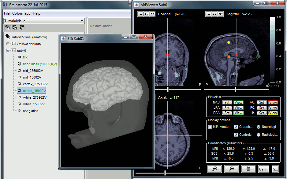
- The two sets of fiducials we usually have to define interactively are here automatically set.
NAS/LPA/RPA: The file Anatomy/Sub01/fiducials.m contains the definition of the nasion, left and right ears. The anatomical points used by the authors are the same as the ones we recommend in the Brainstorm coordinates systems page.
AC/PC/IH: Automatically identified using the SPM affine registration with an MNI template.
If you want to double-check that all these points were correctly marked after importing the anatomy, right-click on the MRI > Edit MRI.
At the end of the process, make sure that the file "cortex_15000V" is selected (downsampled pial surface, that will be used for the source estimation). If it is not, double-click on it to select it as the default cortex surface. Do not worry about the big holes in the head surface, parts of MRI have been remove voluntarily for anonymization purposes.
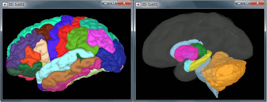
All the anatomical atlases generated by FreeSurfer were automatically imported: the surface-based cortical atlases and the atlas of sub-cortical regions (ASEG).
Access the recordings
Link the recordings
- Switch to the "functional data" view.
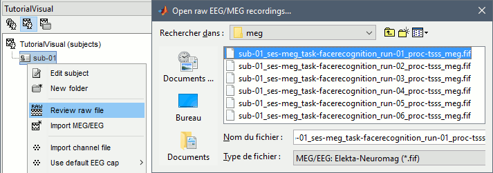
Right-click on the subject folder > Review raw file.
Select the file format: "MEG/EEG: Neuromag FIFF (*.fif)"
Select the first FIF files in: Sub001/MEEG
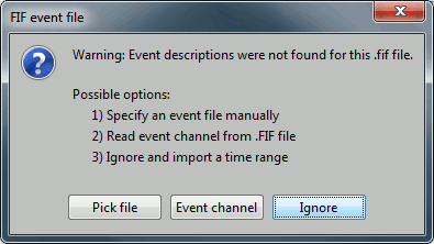
Events: Ignore
We will read events for the stimulus channel and define trial definitions later.
Refine registration now? NO
The head points that are available in the FIF files contain all the points that were digitized during the MEG acquisition, including the ones corresponding to the parts of the face that have been removed from the MRI. If we run the fitting algorithm, all the points around the nose will not match any close points on the head surface, leading to a wrong result. We will first remove the face points and then run the registration manually.
Channel classification
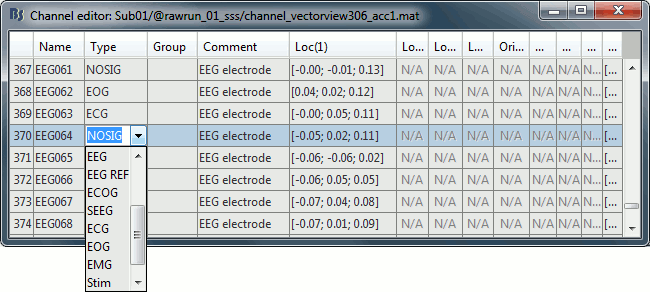
A few non-EEG channels are mixed in with the EEG channels, we need to change this before applying any operation on the EEG channels.
Right-click on the channel file > Edit channel file. Double-click on a cell to edit it.
Change the type of EEG062 to EOG (electrooculogram).
Change the type of EEG063 to ECG (electrocardiogram).
Change the type of EEG061 and EEG064 to NOSIG.
MRI registration
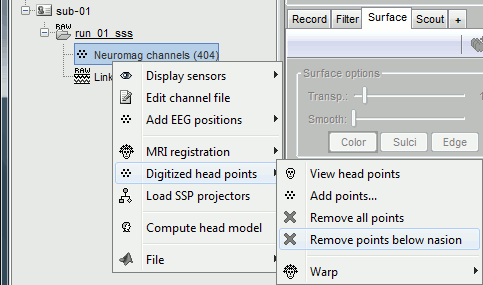
Right-click on the channel file > Digitized head points > Remove points below nasion.
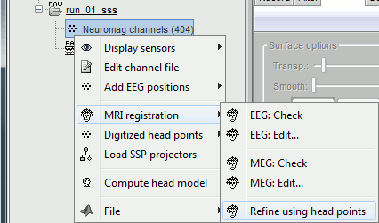
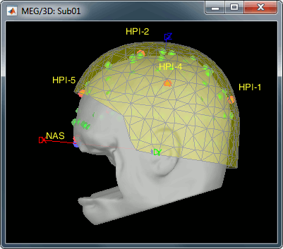
Right-click on the channel file > MRI registration > Refine registration.
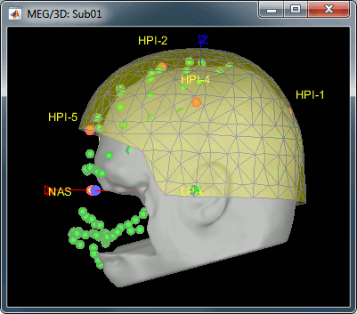
MEG/MRI registration, before (left) and after (right) this automatic registration procedure:
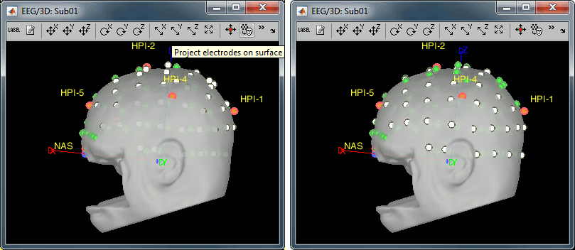
Right-click on the channel file > MRI registration > EEG: Edit...
Click on [Project electrodes on surface]
- Close all the windows (use the [X] button at the top-right corner of the Brainstorm window).
Import event markers
Right-click on the "Link to raw file" > MEG (all) > Display time series.
In the Record tab, menu File > Read events from channel.
- Three event markers represent each trial type that we will explore in this analysis and need to be merged to one event.
In the Record tab, menu Events > Merge groups combine the following events to create the labeled groups:
- Because the detection only looks for values, multiple events can be detected in one trial. For example, a value of 7 represents a Famous trial, but during the trial another event occurred as well. The value went from 7 to 4101, for example, and then back to 7. In this case, the 7 would be counted twice.
In the Record tab, menu Events > Detect multiple responses, remove the extra events
- The stimulus presentation to the subject has a delay of 34.5ms, which can be corrected with an offset.
In the Record tab, menu Events > Add time offset
- Complete these same steps (merge, detect multiple and add time offset) for types Unfamiliar and Scrambled.
Pre-processing
Spectral evaluation
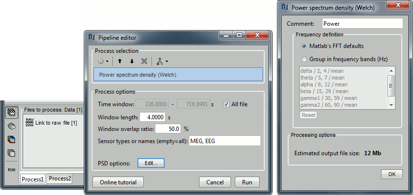
Run process "Frequency > Power spectrum density (Welch)" with the options illustrated below.
Right-click on the PSD file > Power spectrum.
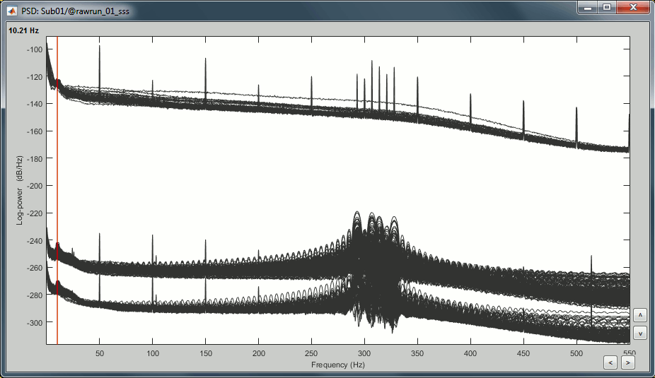
- Observations:
- Three groups of sensors, from top to bottom: EEG, MEG gradiometers, MEG magnetometers.
Power lines: 50 Hz and harmonics
- Alpha peak around 10 Hz
Artifacts due to Elekta electronics: 293Hz, 307Hz, 314Hz, 321Hz, 328Hz.
Suspected bad EEG channels: EEG016
- Close all the windows.
Remove line noise
- Keep the "Link to raw file" in Process1.
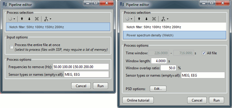
Select process "Pre-process > Notch filter" to remove the line noise (50-200Hz).
Add immediately after the process "Frequency > Power spectrum density (Welch)"
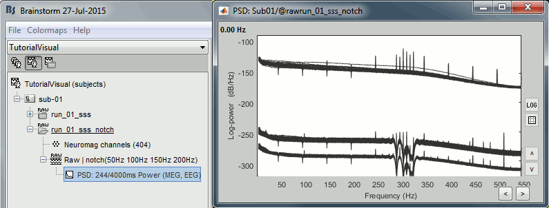
Double-click on the PSD for the new continuous file to evaluate the quality of the correction.
- Close all the windows (use the [X] button at the top-right corner of the Brainstorm window).
EEG reference and bad channels
Right-click on link to the processed file ("Raw | notch(50Hz ...") > EEG > Display time series.
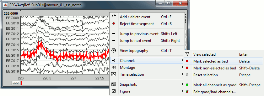
Select channel EEG016 and mark it as bad (using the popup menu or pressing Delete key).
In the Record tab, menu Artifacts > Re-reference EEG > "AVERAGE".
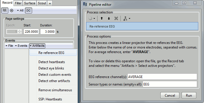
At the end, the window "select active projectors" is open to show the new re-referencing projector. Just close this window. To get it back, use the menu Artifacts > Select active projectors.
Artifact correction with SSP
Artifact detection
In the record tab, run the following menus:
Artifacts > Detect heartbeats: Channel name=EEG063, All file, Event name=cardiac
- In many of the other tutorials, you will have detected the blink category and used the SSP process to remove the blink artifact. In this experiment, we are particularly interested in the subject's response to seeing the stimulus. Therefore we will mark eyeblinks and other eye movements as BAD.
Artifacts > Detect events above threshold: Channel name=EEG062, All file, Event name=blink_BAD, Maximum threshold=100, Threshold units=uV, Filter=[0.30,20.00]Hz, Use absolute value is checked
![[ATTACH] [ATTACH]](/moin_static1911/brainstorm1/img/attach.png)
![[ATTACH] [ATTACH]](/moin_static1911/brainstorm1/img/attach.png)
- Close all the windows (using the [X] button).
Heartbeats
Empty the Process1 list (right-click > Clear list).
- Drag and drop the continuous processed file ("Raw | notch(50Hz...)") to the Process1 list.
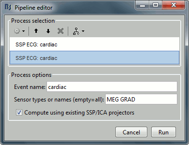
- Select the following processes and run the pipeline:
Artifacts > SSP: Heartbeats > Sensor type: MEG MAG
Artifacts > SSP: Heartbeats > Sensor type: MEG GRAD
Double-click on the continuous file to show all the MEG sensors.
In the Record tab, select sensors "Left-temporal".Menu Artifacts > Select active projectors.
In category cardiac/MEG MAG: Select component #1 and view topography.
In category cardiac/MEG GRAD: Select component #1 and view topography.

Make sure that selecting the two components removes the cardiac artifact. Then click [Save].
Additional bad segments
Process1>Run: Select the process "Events > Detect other artifacts". This should be done separately for MEG and EEG to avoid confusion about which sensors are involved in the artifact.
![[ATTACH] [ATTACH]](/moin_static1911/brainstorm1/img/attach.png)
Display the MEG sensors. Review the segments that were tagged as artifact, determine if each event represents an artifact and then mark the time of the artifact as BAD. This can be done by selecting the time window around the artifact, Right-click > Reject time segment. Note that this detection process marks 1-second segments but the artifact can be shorter.

- Once all the events in the two categories are reviewed and bad segments are marked, the two categories (1-7Hz and 40-240Hz) can be deleted.
- Do this detection and review again for the EEG.
SQUID SENSOR ARTIFACTS (SQUID JUMPS): Because of the different sensor technologies, one can expect that the different MEG systems may produce different types of artifact. With the Neuromag system, used for this experiment, one can see an artifact produced by the sensors which is exaggerated by the pre-processing completed with Max Filter, seen here in the examples below. The spacial filtering of Max Filter causes the artifact to be speard across most sensors and also spread a bit in time. Ideally, the offending should be marked bad before applying the Max Filter. In the case of this dataset, we have the artifacts - sometimes more frequent than others. The 1-7Hz artifact detection employed here will usually catch them, but it is important to review all the sensors and all the time in each recording to be sure these events are marked as bad segments.
![[ATTACH] [ATTACH]](/moin_static1911/brainstorm1/img/attach.png)
![[ATTACH] [ATTACH]](/moin_static1911/brainstorm1/img/attach.png)
Prepare all runs
Complete the above steps for Runs 2-6:
Access the recordings
Pre-processing
Artifact detection
Epoching and averaging
Import epochs
Drag and drop the 6 pre-processed raw folders in Process1 > Run
Run the two processes together: Import recordings > Import MEG/EEG: Events and Pre-process > Remove DC offset
![[ATTACH] [ATTACH]](/moin_static1911/brainstorm1/img/attach.png)
![[ATTACH] [ATTACH]](/moin_static1911/brainstorm1/img/attach.png)
![[ATTACH] [ATTACH]](/moin_static1911/brainstorm1/img/attach.png)
Average
- Drag and drop all the imported trials in Process1.
Run > Average > Average files: By trial groups (folder average)
![[ATTACH] [ATTACH]](/moin_static1911/brainstorm1/img/attach.png)
![[ATTACH] [ATTACH]](/moin_static1911/brainstorm1/img/attach.png)
Review EEG ERP
- Make a cluster with channel EEG065 and overlay the channel across the three conditions.
Select the cluster then select three average files and right click > Clusters time series
![[ATTACH] [ATTACH]](/moin_static1911/brainstorm1/img/attach.png)
![[ATTACH] [ATTACH]](/moin_static1911/brainstorm1/img/attach.png)
- Around 170ms (N170) there is a greater negative deflection for Famous than Scrambled faces and as well as a difference between Famous and Unfamiliar faces after 250ms.
Empty room recordings
For this dataset, one empty room recording will be used for all subjects.
Create a new subject: emptyroom
Create a link to the raw file: sample_group/EmptyRoom/090707.fif
Apply the same notch filter as for the data
Compute the noise covariance. Right-click on Raw | notch > Noise covariance > Compute from recordings
Copy the noise covariance to Sub001. Right-click on the Noise covariance > Copy to other subjects
![[ATTACH] [ATTACH]](/moin_static1911/brainstorm1/img/attach.png)
Source estimation
MEG
- Head Model: We will compute one head model file which contains both the Overlapping Spheres (MEG) model and OpenMEEG BEM (EEG) model. To compute the OpenMEEG BEM on the EEG, it is necessary to prepare the BEM surfaces.
Switch to the "Anatomy" view. Right-click on Sub01 > Generate BEM surfaces. Select the default values. If you have memory errors while generating the model (below), you can reduce the number of vertices in these BEM surfaces.
![[ATTACH] [ATTACH]](/moin_static1911/brainstorm1/img/attach.png)
- Switch back to the "Functional" view. Drag and drop the 6 imported trial folders in Process1.
Run > Sources > Compute head model: Overlapping spheres (MEG) and OpenMEEG BEM (EEG). It will take quite a long time to compute the BEM models.
Source Model: Run > Sources > Compute sources, Sensor types=MEG, Leave all the default options to calculate a wMNE solution with constrained dipole orientation.
Averaging
Drag and drop all the imported trials in Process1, be sure to select the file type sources. Stack all the following processes to select a uniform number of trials, average across runs, filter, extract time and normalize:
File > Select uniform number of trials: By trial group (subject), Uniformly distributed
Average > Average files: By trial groups (subject average)
Pre-process > Band-pass filter: Lower cutoff=0, Upper cutoff=32
Extract > Extract time: Time window [-100,800]Hz
Standardize > Z-score normalization: Baseline=[-100,-1]ms, uncheck Use absolute values and uncheck Dynamic
![[ATTACH] [ATTACH]](/moin_static1911/brainstorm1/img/attach.png)
MEG source maps at 170ms, Famous, Scrambled, Unfamiliar:

Plot the activation over time limited to the fusiform.
In the Scout panel, select the Desikan-Killiany atlas from the dropdown menu.
Select the two scouts: LT fusiform and RT fusiform
Plot the two scout time series, with relative values, overlaying the conditions
![[ATTACH] [ATTACH]](/moin_static1911/brainstorm1/img/attach.png)
EEG
- Compute a EEG noise covariance for EACH RUN using the EEG recordings and merge it with the existing noise covariance, which contains the noise covariance for MEG.
Expand the folder run_01_sss_notch to see the imported files. Select all imported trials, Right-click > Noise covariance > Compute from recordings, Time window=[-300,0]ms, Sensor types=EEG, select Merge.
- Repeat for runs 2-6.
Run > Sources > Compute sources, Sensor types=EEG, Leave all the default options to calculate a wMNE solution with constrained dipole orientation. Click Run.
Average the EEG sources: Drag and drop all the imported trials in Process1, be sure to select the file type sources and apply a filter: EEG (to select only the EEG sources). Stack all the following processes to select a uniform number of trials, average across runs, filter, extract time and normalize:
File > Select uniform number of trials: By trial group (subject), Uniformly distributed
Average > Average files: By trial groups (subject average)
Pre-process > Band-pass filter: Lower cutoff=0, Upper cutoff=32
Extract > Extract time: Time window [-100,800]Hz
Standardize > Z-score normalization: Baseline=[-100,-1]ms, uncheck Use absolute values and uncheck Dynamic
Scripting
Corresponding script in the Brainstorm distribution:
TODO: Coming soon.
