|
Size: 8726
Comment:
|
Size: 9720
Comment:
|
| Deletions are marked like this. | Additions are marked like this. |
| Line 2: | Line 2: |
| ''Author: Seyed-Mahdi Khaligh-Razavi'' | ''Author: Seyed-Mahdi Khaligh-Razavi, Francois Tadel, and Dimitrios Pantazis'' |
| Line 4: | Line 4: |
| These set of functions allow you to do support vector machine (SVM) and linear discriminant analysis (LDA) classification on your MEG data across time. | This set of functions allow you to do support vector machine (SVM) and linear discriminant analysis (LDA) classification on your MEG data across time. |
| Line 13: | Line 13: |
| During MEG recordings participants completed an orthogonal image categorization task. Participants saw 720 stimuli (360 faces, 360 scenes) centrally-presented ( 6 degree visual angle) for 0.5 second at a time and had to decide (without responding) if scenes were indoor / outdoor and faces were male / female. Every 2 to 4 trials (randomly determined), a question mark would appear on the screen for 1 second. At this time, participants were asked to press a button to indicate the category of the last image (male/female, indoor/outdoor), and they were also allowed to blink/swallow. This task was designed to ensure participants were attentive to the images without explicitly encoding them into memory. Participants only responded during the “question mark” trials so that activity during stimulus perception was not contaminated by motor activity. During the task, participants were asked to fixate on a cross centered on the screen and their eye movements were tracked, to ensure any results were not due to differential eye movement patterns. The whole experiment was divided into 16 runs. Each run contained 45 randomly selected images (each of them shown twice per run—not in succession), resulting in a total experiment time of about 50 min. The MEG data that is included here for demonstration purposes contains only the first 15 minutes of the whole session, during which 53 faces and 54 scenes have been observed. | During MEG recordings participants completed an orthogonal image categorization task. Participants saw 720 stimuli (360 faces, 360 scenes) centrally-presented ( 6 degree visual angle) for 0.5 second at a time and had to decide (without responding) if scenes were indoor / outdoor and faces were male / female. Every 2 to 4 trials (randomly determined), a question mark would appear on the screen for 1 second. At this time, participants were asked to press a button to indicate the category of the last image (male/female, indoor/outdoor), and they were also allowed to blink/swallow. This task was designed to ensure participants were attentive to the images without explicitly encoding them into memory. Participants only responded during the “question mark” trials so that activity during stimulus perception was not contaminated by motor activity. During the task, participants were asked to fixate on a cross centered on the screen and their eye movements were tracked, to ensure any results were not due to differential eye movement patterns. The whole experiment was divided into 16 runs. Each run contained 45 randomly selected images (each of them shown twice per run—not in succession), resulting in a total experiment time of about 50 min. <<BR>>The MEG data that is included here for demonstration purposes contains only the first 15 minutes of the whole session, during which 53 faces and 54 scenes have been observed. == License == This MEG decoding dataset remains a property of Aude Oliva’s Lab, Computer Science and AI (CSAIL), Massachusetts Institute of Technology, Cambridge, US. Its use and transfer outside the Brainstorm tutorial, e.g. for research purposes, is prohibited without written consent from the Lab. If you reference this dataset in your publications, please acknowledge its authors (Seyed-Mahdi Khaligh-Razavi, Francois Tadel, and Dimitrios Pantazis) and cite Khaligh-Razavi et al. (2015) and Brainstorm as indicated on the [[http://neuroimage.usc.edu/brainstorm/CiteBrainstorm|website]]. For questions, please contact us through the forum. |
| Line 93: | Line 100: |
== References == 1. Khaligh-Razavi, S-M; Bainbridge, W; Pantazis, D; and Oliva, A. (2015) Introducing Brain Memorability: an MEG study (in preparation). 1. Cichy, R.M., Pantazis, D., and Oliva, A. (2014). Resolving human object recognition in space and time. Nat Neurosci 17, 455–462. |
Tutorial 13: Decoding Conditions
Author: Seyed-Mahdi Khaligh-Razavi, Francois Tadel, and Dimitrios Pantazis
This set of functions allow you to do support vector machine (SVM) and linear discriminant analysis (LDA) classification on your MEG data across time.
Contents
Description of the MEG data
The data contains the first 15 minutes of MEG recording for one of the subjects in the following study, and can be downloaded from here: https://www.dropbox.com/s/fmu5p3950e2mknc/mem6-0_tsss_mc.fif?dl=0
The study was conducted according to the Declaration of Helsinki and approved by the local ethics committee (Institutional Review Board of the Massachusetts Institute of Technology). Informed consent was obtained from all participants.
During MEG recordings participants completed an orthogonal image categorization task. Participants saw 720 stimuli (360 faces, 360 scenes) centrally-presented ( 6 degree visual angle) for 0.5 second at a time and had to decide (without responding) if scenes were indoor / outdoor and faces were male / female. Every 2 to 4 trials (randomly determined), a question mark would appear on the screen for 1 second. At this time, participants were asked to press a button to indicate the category of the last image (male/female, indoor/outdoor), and they were also allowed to blink/swallow. This task was designed to ensure participants were attentive to the images without explicitly encoding them into memory. Participants only responded during the “question mark” trials so that activity during stimulus perception was not contaminated by motor activity. During the task, participants were asked to fixate on a cross centered on the screen and their eye movements were tracked, to ensure any results were not due to differential eye movement patterns. The whole experiment was divided into 16 runs. Each run contained 45 randomly selected images (each of them shown twice per run—not in succession), resulting in a total experiment time of about 50 min.
The MEG data that is included here for demonstration purposes contains only the first 15 minutes of the whole session, during which 53 faces and 54 scenes have been observed.
License
This MEG decoding dataset remains a property of Aude Oliva’s Lab, Computer Science and AI (CSAIL), Massachusetts Institute of Technology, Cambridge, US. Its use and transfer outside the Brainstorm tutorial, e.g. for research purposes, is prohibited without written consent from the Lab.
If you reference this dataset in your publications, please acknowledge its authors (Seyed-Mahdi Khaligh-Razavi, Francois Tadel, and Dimitrios Pantazis) and cite Khaligh-Razavi et al. (2015) and Brainstorm as indicated on the website. For questions, please contact us through the forum.
Description of the decoding functions
These set of functions allow you to do support vector machine (SVM) and linear discriminant analysis (LDA) classification on your MEG data across time.
Input: the input is channel data from two conditions (e.g. condA and condB) across time. Number of samples per condition should be the same for both condA and condB. Each of them should at least contain two samples.
Output: the output is a decoding curve across time, showing your decoding accuracy (decoding condA vs. condB) at timepoint 't'.
We have two condition types: faces, and scenes. We want to decode faces vs. scenes using 306 MEG channels. In the data, the faces are named as condition ‘201’; and the scenes are named as condition ‘203’.
Creating protocol and loading the data
Go to the file menu and create a new protocol called faces_vs_scenes with the options shown in the following figure.
After making your protocol, go to the functional data view (sorted by subjects). Then create a new subject (let's keep the default name: Subject01): to create a new subject right click on the protocol name; then press new subject, choose the default values shown in the following figure; press save.
Import MEG data
Right click on the subject node (Subject01), and select ‘review raw file’.
Change the file format to ‘MEG/EEG: Neuromag FIF (*.fif)’; then select the .fif file (mem6-0_tsss_mc.fif) you downloaded.
Press event channels
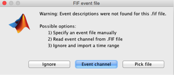
In the ‘mem6-0 tsss mc’ node right click on ‘Link to raw file’; select ‘Import in database’.
- Set epoch time to [-100, 1000]
- Time range: [-100,0]
From the events select only these two events: 201 (faces), and 203(scenes)
![[ATTACH] [ATTACH]](/moin_static1911/brainstorm1/img/attach.png)
- Then press import. You will get a message saying ‘some epochs are shorter than the others..’ . Press yes.
Decoding conditions
- Select ‘Process2’ from the bottom brainstorm window.
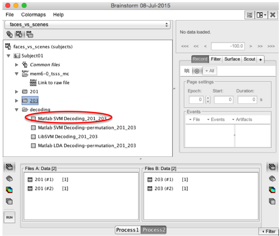
Drag and drop 40 files from folder ‘201’ to ‘Files A’; and 40 files from folder ‘203’ to ‘Files B’. You can select more than 40 or less. The important thing is that both ‘A’ and ‘B’ should have the same number of files.
![[ATTACH] [ATTACH]](/moin_static1911/brainstorm1/img/attach.png)
a) Cross-validation
Cross-validation is a model validation technique for assessing how the results of our decoding analysis will generalize to an independent data set.
Select run -> decoding conditions -> classification with cross validation
![[ATTACH] [ATTACH]](/moin_static1911/brainstorm1/img/attach.png)
Here, you will have three choices for cross-validation. If you have Matlab Statistics and Machine Learning Toolbox, you can use ‘Matlab SVM’ or ‘Matlab LDA’. You can also install the ‘LibSVM’ toolbox (https://www.csie.ntu.edu.tw/~cjlin/libsvm/ ); and addpath it to your Matlab session. LibSVM may be faster. The LibSVM cross-validation won’t be stratified. However, if you select Matlab SVM/LDA, it will do a k-fold stratified cross-validation for you, meaning that each fold will contain the same proportions of the two types of class labels.
You can also set the number of folds for cross-validation; and the cut-off frequency for low-pass filtering – this is to smooth your data.
2- To continue, set the values as shown below:
![[ATTACH] [ATTACH]](/moin_static1911/brainstorm1/img/attach.png)
3- The process will take some time.The results are then saved in a file (‘Matlab SVM Decoding_201_203’) under the new ‘decoding’ node. If you double click on it you will see a decoding curve across time (shown below).
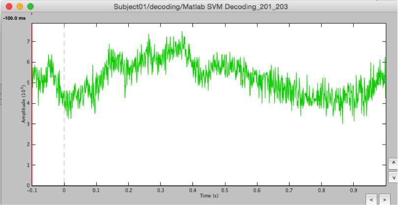
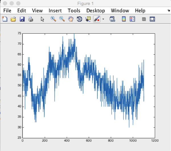
The internal brainstorm plot is not perfect for this purpose. To make a proper plot you can plot the results yourself. Right click on the result file (Matlab SVM Decoding_201_203), select 'export to Matlab' from the menu. Give it a name ‘decodingcurve’. Then using Matlab plot function you can plot the decoding accuracies across time.
Matlab code:
figure;
plot(decodingcurve.Value);
b) Permutation
This is an iterative procedure. The training and test data for the SVM/LDA classifier are selected in each iteration by randomly permuting the samples and grouping them into bins of size n (you can select the trial bin sizes). In each iteration two samples (one from each condition) are left out for test. The rest of the data are used to train the classifier with.
Select run -> decoding conditions -> classification with permutation
- Set the values as the following:
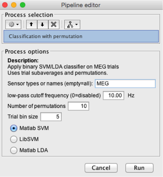
If the ‘Trial bin size’ is greater than 1, the training data will be randomly grouped into bins of the size you determine here. The samples within each bin are then averaged (we refer to this as sub-averaging); the classifier is then trained using the averaged samples. For example, if you have 40 faces and 40 scenes, and you set the trial bin size to 5; then for each condition you will have 8 bins each containing 5 samples. Seven bins from each condition will be used for training, and the two left-out bins (one face bin, one scene bin) will be used for testing the classifier performance.
- 3- The results are saved under the ‘decoding ’ node . If you selected ‘Matlab SVM’, the file name will be ‘Matlab SVM Decoding-permutation_201_203’ . Double click on it. You will get the plot blow:
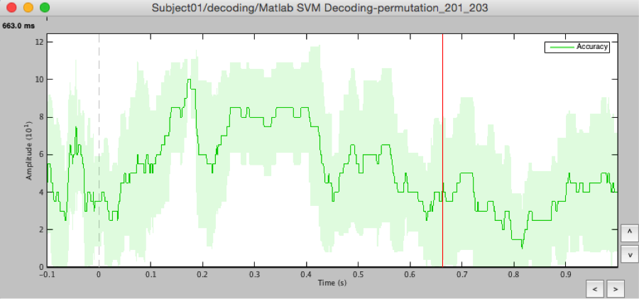
This might not be very intuitive. You can export the decoding results into Matlab and plot it yourself. If you export the decoding results into Matlab, the imported structure will have two important fields:
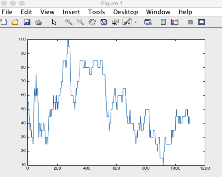
- a) Value: this is the mean decoding accuracy across all permutations
- b) Std: this is the standard deviation across all permutations.
If you plot the mean value (decodingcurve.Value), below is what you will get. You also have access to the standard deviation (decodingcurve.Std), in case you want to plot it.
References
- Khaligh-Razavi, S-M; Bainbridge, W; Pantazis, D; and Oliva, A. (2015) Introducing Brain Memorability: an MEG study (in preparation).
- Cichy, R.M., Pantazis, D., and Oliva, A. (2014). Resolving human object recognition in space and time. Nat Neurosci 17, 455–462.
