|
Size: 36
Comment:
|
Size: 11602
Comment:
|
| Deletions are marked like this. | Additions are marked like this. |
| Line 1: | Line 1: |
| Describe Tutorials/DeepAtlas here. | = DBA tutorial: Compute sources in deep cerebral structures = ''Authors: Jean-Eudes Le Douget, Francois Tadel, Denis Schwartz'' This tutorial explains step-by-step how to use the DBA (Deep Brain Activity) functionality, useful to assess subcortical source localization. <<TableOfContents(2,2)>> == Import database == This tutorial is based on resting-state recordings for 7 subjects with two conditions: eyes open (YO), eyes closed (YF). We have recorded 20 runs of 15 seconds for each subject and each condition. The goal is to compute the contrast between the two conditions in the alpha band. The data has already been filtered in the alpha frequency band (7-13Hz) and the default anatomy is used for all the subjects. * Start by downloading the tutorial dataset '''TutorialDba.zip''' from the [[http://neuroimage.usc.edu/bst/download.php|Download]] page. * The file is an exported Brainstorm protocol. To load it in your database, use the menu:<<BR>> File > Load Protocol > '''Load from zip file'''. <<BR>><<BR>> {{attachment:loadzip.gif}} == Select deep structures == The first step consists in creating the surface file that includes the cortex and the deep structures that we want to include in the model. Here, in the default anatomy: * Right-click on "aseg atlas" > '''Less vertices''' > '''15000''' vertices. <<BR>><<BR>> {{attachment:aseg_downsample.gif||height="213",width="436"}} * Double-click on "aseg atlas_15000V" (contains the subcortical structures from the FreeSurfer altas). * Select the amygdala, the thalamus and the hippocampus, and create a subatlas. <<BR>><<BR>> {{attachment:aseg_keep.gif||height="385",width="555"}} * '''Merge '''the cortex with the selected structures. '''Rename '''the new surface in "cortex_mixed". <<BR>><<BR>> {{attachment:aseg_merge.gif}} {{attachment:aseg_rename.gif}} * Open the cortex_mixed surface and create a new atlas "'''Source model options'''". With Matlab 2015b+, the display looks weird because it limits the number of possible transparent layers to 5. To produce nicer figures, disable the OpenGL renderer (File > Edit preferences). The display will be much slower, but the renderer won't suffer from this limitation.<<BR>><<BR>> {{attachment:atlas_model.gif||height="214",width="668"}} * Set the set modeling options to "'''Deep brain'''" for all the structures.<<BR>><<BR>> {{attachment:atlas_dba.gif||height="246",width="606"}} == Location and orientation constraints == Two types of constraints can be applied to each anatomical region in the atlas "Source model": * '''Location constraint''': Defines where the sources corresponding to these regions are placed. * '''Surface''': The sources are located on the surface of the structure (cortex and hippocampus). The surface describing the region is directly used as the source space. * '''Volume''': The sources are located inside the volume of the region. The source space is a grid of points uniformly distributed inside of the volume delimited by the syrface of the structure. * '''Deep brain''': Use the preferred configuration defined in the Deep Brain Atlas (surface for the cerebral cortex and hippocampus, volume for all the other structures). * '''Orientation constraint''': * '''Constrained''': Defines only one dipole per grid point, with a fixed orientation orientation. * With option "Surface": Uses the normal orientation to the surface at each point. * With option "Deep brain": Uses the preferred orientation defined in the atlas (see below). * '''Unconstrained''': Uses three orthogonal dipoles per grid point (x,y,z). * '''Loose''': Intermediate option, uses three orthogonal dipoles per grid point, but favors the preferred orientation used for the contrained case. Based on the anatomical observations reported for each subcortical region in the reference articles (next section), the preferred combination of constrains is described below.<<BR>><<BR>> || ||'''Location constraint''' ||'''Preferred orientation''' ||'''Default''' || ||'''Cortex''' ||Surface ||Normal ||Constrained || ||'''Hippocampus''' ||Surface ||Normal ||Constrained || ||'''Cerebellum''' ||Surface ||Normal ||Unconstrained || ||'''Accumbens''' ||Volume ||None ||Unconstrained || ||'''Amygdala ||Volume ||None ||Unconstrained || ||'''Brainstem''' ||Volume ||None ||Unconstrained || ||'''Caudate''' ||Volume ||None ||Unconstrained || ||'''Putamen''' ||Volume ||None ||Unconstrained || ||'''Pallidum''' ||Volume ||Y axis ||Constrained || ||'''Thalamus''' ||Volume ||None ||Unconstrained || * '''Cortex''': Surface / Normal orientation * '''Hippocampus''': Surface / Normal orientation * '''Cerebellum''': Surface / Normal orientation * '''Accumbens''': Volume / Random orientation * '''Amygdala''': Volume / Random orientation * '''Brainstem''': Volume / Random orientation (Unconstrained orientation preferred) * '''Caudate''': Volume / Random orientation (Unconstrained orientation preferred) * '''Putamen''': Volume / Random orientation (Unconstrained orientation preferred) * . case {'Pallidum L','LEgp', 'LIgp','Pallidum R','REgp', 'RIgp'} . regionType = 'vol'; regionOrient = 'y'; . case {'Thalamus L','LTha','Thalamus R','RTha'} . regionType = 'vol'; regionOrient = 'random'; case {'lh', '01_Lhemi L', 'Cortex L', 'rh', '01_Rhemi R', 'Cortex R'} Describe the constraints applied to each region. == Source estimation [TODO] == ==== Head model ==== * Select all the subjects (except for the empty room recordings) > right-click > '''Compute head model'''. Select "'''Custom source model'''", and leave the other options to their defaults. <<BR>><<BR>> {{attachment:dba_headmodel.gif||height="244",width="443"}} * You can explore the source grids that were computed. Right-click on one of the head models > '''Check source grid (volume)''' and '''Check source grid (surface)'''. In the Scout tab, select the atlas "User scouts" to get a clearer view. In panel Surface, increase the transparency of the surface to see the source grids representing the select subcortical regions. <<BR>><<BR>> {{attachment:headmodel_grid.gif||height="198",width="665"}} ==== Inverse model ==== * The noise covariance matrix was estimated from the empty room recordings (Empty_Subject) and copied to all the folders of all the subjects. * Select all the subjects (except the empty room recordings), right-click > '''Compute sources'''. <<BR>>Select '''Minimum norm (wMNE)''' and lelave the other options to their default values. <<BR>><<BR>> {{attachment:dba_inverse.gif||height="235",width="446"}} * Double-click on the sources for any trial (segment of 15s of rest recordings). Make sure the atlas "'''User scouts'''" is selected in the Scout tab, then explore the display options available in the Surface tab. The surface regions (cortex and hippocampus) are represented as surfaces, and the values are directly mapped on the surface. The volume regions (amygdala and thalamus) are represented as grids of dots. <<BR>><<BR>> {{attachment:dba_display.gif||height="244",width="647"}} * In the Scout tab, you can use the atlas "'''Source model'''" to display separately some regions difficult to observe with all the cortex. Typically the activity on the hippocampus surface. Click on the button [SEL] to display only the selected regions, then select the hippocampus entries. [TODO] == Compute statistics == We will now design a statistical analysis to assess the eyes-open and eyes-closed contrast. As a reminder, the recordings available in the database have already been filtered in the alpha frequency band (7-13Hz). As a measure of the global of the activity in this frequency band, we will average all the time samples in each block of 15s. Note that this is not the recommended procedure anymore: it would have been better to simply compute a PSD from the sources estimated for the continuous file link, but this option was not available at the time this tutorial was written. * In Process1, select all the subjects (except for Empty_Subject)and select '''[Process sources]'''. * Run process Average > '''Average time''' > Use absolute value, All file. <<BR>><<BR>> {{attachment:dba_avgtime.gif}} * * Then, the "Process2" tab is used : place the source power files of the eyes-closed condition in the "Files A" space and of the eyes-open condition in the "Files B" space.<<BR>>To gain time, it is possible to sort the functional data by conditions, place the subjects in "FilesA" and "FilesB" and use the filter to include only files that contain 'avg' (for time-averaged files) * Run a Student's T-Test to compute a statistical contrast between the conditions<<BR>><<BR>> {{attachment:DBA_Ttest.png||height="422",width="383"}} {{attachment:DBA_TtestOptions.png||height="283",width="226"}} * The stat file can then be visualized and the values corresponding to subcortical structures are also appearing<<BR>><<BR>> {{attachment:DBA_VisuStat.png||height="286",width="523"}} * It is also interesting to observe the difference of means between conditions. To compute this, instead of runnning a Student's T-Test, select the "Difference of means" option<<BR>><<BR>> {{attachment:DBA_DiffOfMeans.png||height="283",width="394"}} == Volume scouts == Some subcortical structures are modeled as volume source structures (for instance here, the thalamus and the amygdala). It is not possible to display scouts time series for these structures from the "Source model" or "Structures" atlases. It is necessary to create a new atlas, specific to volume scouts. The steps are the following : * First, create the volume atlas<<BR>><<BR>> {{attachment:DBA_VolumeScouts.png||height="264",width="668"}} * Second, to create a new scout : * Click on the "Create scout" cross, and click one point of the structure you want to include in the scout<<BR>> {{attachment:DBA_VolumeScout_FirstPoint.png||height="291",width="659"}} * Click on the "Increase scout size" as many times as necessary to include all the points of the volume, for example in the right thalamus<<BR>> {{attachment:DBA_IncreaseScoutSize2.png||height="239",width="148"}} {{attachment:DBA_Scout_RightThal.png||height="272",width="266"}} * Rename the scout and set the correct region and the desired function<<BR>><<BR>> {{attachment:DBA_RenameScout.png||height="78",width="192"}} {{attachment:DBA_SetRegion2.png||height="271",width="260"}} {{attachment:DBA_SetFunction2.png||height="270",width="244"}} * Repeat this operation for all the volume scouts you want to create * Finally, you can display time series of your choice<<BR>><<BR>> {{attachment:DBA_DispolayScoutsTS.png||height="306",width="280"}} == References == Attal Y, Bhattacharjee M, Yelnik J, Cottereau B, Lefèvre J, Okada Y, Bardinet E, Chupin M, Baillet S (2009)<<BR>>[[http://www.ncbi.nlm.nih.gov/pubmed/18003114|Modelling and detecting deep brain activity with MEG and EEG]]<<BR>>'''IRBM''', 30(3):133-138 Attal Y, Schwartz D (2013)<<BR>>[[http://www.plosone.org/article/info:doi/10.1371/journal.pone.0059856|Assessment of Subcortical Source Localization Using Deep Brain Activity Imaging Model with Minimum Norm Operators: A MEG Study]]<<BR>>'''PLOS ONE''', 8(3):e59856 Dumas T, Dubal S, Attal Y, Chupin M, Jouvent R (2013)<<BR>>[[http://www.plosone.org/article/info:doi/10.1371/journal.pone.0074145|MEG Evidence for Dynamic Amygdala Modulations by Gaze and Facial Emotions]]<<BR>>'''PLOS ONE''', 8(9): e74145 |
DBA tutorial: Compute sources in deep cerebral structures
Authors: Jean-Eudes Le Douget, Francois Tadel, Denis Schwartz
This tutorial explains step-by-step how to use the DBA (Deep Brain Activity) functionality, useful to assess subcortical source localization.
Contents
Import database
This tutorial is based on resting-state recordings for 7 subjects with two conditions: eyes open (YO), eyes closed (YF). We have recorded 20 runs of 15 seconds for each subject and each condition.
The goal is to compute the contrast between the two conditions in the alpha band. The data has already been filtered in the alpha frequency band (7-13Hz) and the default anatomy is used for all the subjects.
Start by downloading the tutorial dataset TutorialDba.zip from the Download page.
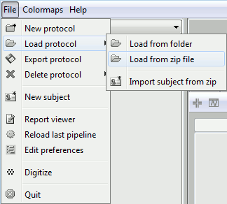
The file is an exported Brainstorm protocol. To load it in your database, use the menu:
File > Load Protocol > Load from zip file.
Select deep structures
The first step consists in creating the surface file that includes the cortex and the deep structures that we want to include in the model. Here, in the default anatomy:
Right-click on "aseg atlas" > Less vertices > 15000 vertices.
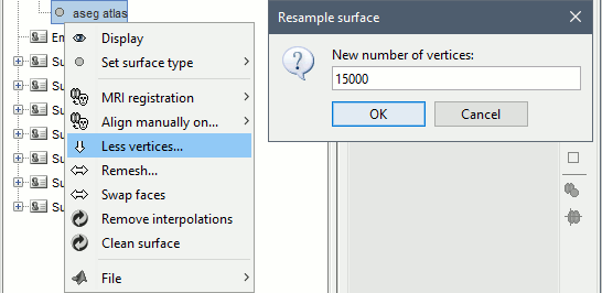
Double-click on "aseg atlas_15000V" (contains the subcortical structures from the FreeSurfer altas).
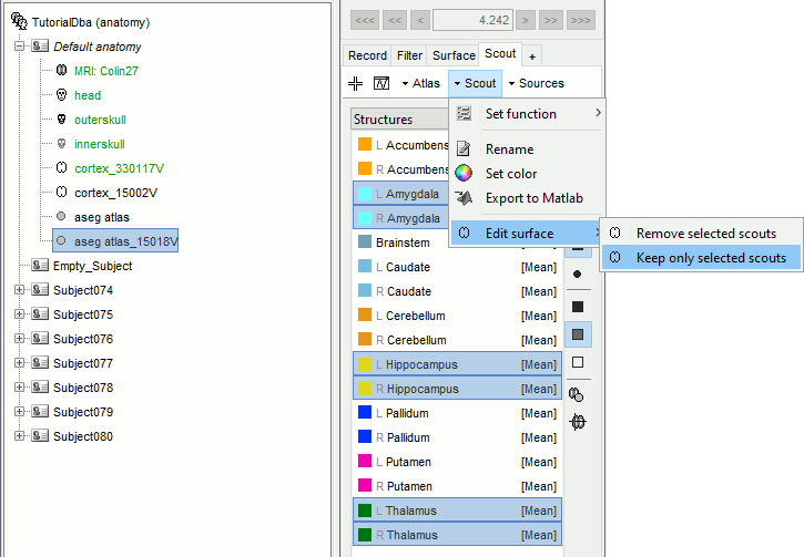
Select the amygdala, the thalamus and the hippocampus, and create a subatlas.
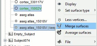
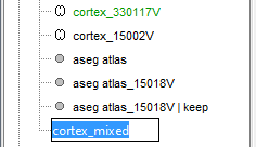
Merge the cortex with the selected structures. Rename the new surface in "cortex_mixed".
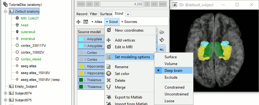
Open the cortex_mixed surface and create a new atlas "Source model options". With Matlab 2015b+, the display looks weird because it limits the number of possible transparent layers to 5. To produce nicer figures, disable the OpenGL renderer (File > Edit preferences). The display will be much slower, but the renderer won't suffer from this limitation.

Set the set modeling options to "Deep brain" for all the structures.
Location and orientation constraints
Two types of constraints can be applied to each anatomical region in the atlas "Source model":
Location constraint: Defines where the sources corresponding to these regions are placed.
Surface: The sources are located on the surface of the structure (cortex and hippocampus). The surface describing the region is directly used as the source space.
Volume: The sources are located inside the volume of the region. The source space is a grid of points uniformly distributed inside of the volume delimited by the syrface of the structure.
Deep brain: Use the preferred configuration defined in the Deep Brain Atlas (surface for the cerebral cortex and hippocampus, volume for all the other structures).
Orientation constraint:
Constrained: Defines only one dipole per grid point, with a fixed orientation orientation.
- With option "Surface": Uses the normal orientation to the surface at each point.
- With option "Deep brain": Uses the preferred orientation defined in the atlas (see below).
Unconstrained: Uses three orthogonal dipoles per grid point (x,y,z).
Loose: Intermediate option, uses three orthogonal dipoles per grid point, but favors the preferred orientation used for the contrained case.
Based on the anatomical observations reported for each subcortical region in the reference articles (next section), the preferred combination of constrains is described below.
Location constraint
Preferred orientation
Default
Cortex
Surface
Normal
Constrained
Hippocampus
Surface
Normal
Constrained
Cerebellum
Surface
Normal
Unconstrained
Accumbens
Volume
None
Unconstrained
Amygdala
Volume
None
Unconstrained
Brainstem
Volume
None
Unconstrained
Caudate
Volume
None
Unconstrained
Putamen
Volume
None
Unconstrained
Pallidum
Volume
Y axis
Constrained
Thalamus
Volume
None
Unconstrained
Cortex: Surface / Normal orientation
Hippocampus: Surface / Normal orientation
Cerebellum: Surface / Normal orientation
Accumbens: Volume / Random orientation
Amygdala: Volume / Random orientation
Brainstem: Volume / Random orientation (Unconstrained orientation preferred)
Caudate: Volume / Random orientation (Unconstrained orientation preferred)
Putamen: Volume / Random orientation (Unconstrained orientation preferred)
- . case {'Pallidum L','LEgp', 'LIgp','Pallidum R','REgp', 'RIgp'}
- regionType = 'vol'; regionOrient = 'y';
- case {'Thalamus L','LTha','Thalamus R','RTha'}
- regionType = 'vol'; regionOrient = 'random';
Describe the constraints applied to each region.
Source estimation [TODO]
Head model
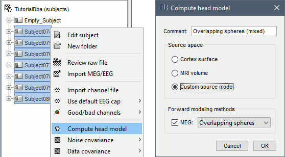
Select all the subjects (except for the empty room recordings) > right-click > Compute head model. Select "Custom source model", and leave the other options to their defaults.
You can explore the source grids that were computed. Right-click on one of the head models > Check source grid (volume) and Check source grid (surface). In the Scout tab, select the atlas "User scouts" to get a clearer view. In panel Surface, increase the transparency of the surface to see the source grids representing the select subcortical regions.

Inverse model
- The noise covariance matrix was estimated from the empty room recordings (Empty_Subject) and copied to all the folders of all the subjects.
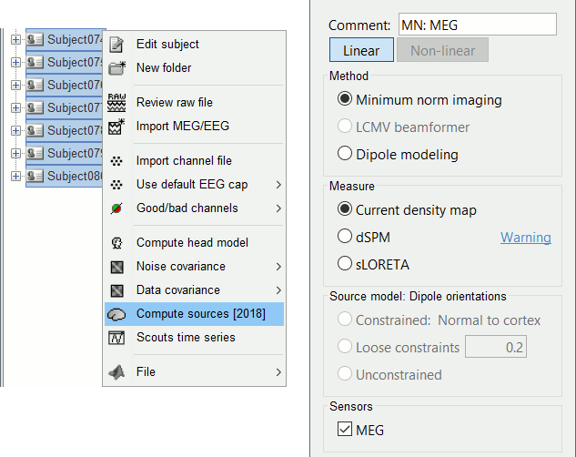
Select all the subjects (except the empty room recordings), right-click > Compute sources.
Select Minimum norm (wMNE) and lelave the other options to their default values.
Double-click on the sources for any trial (segment of 15s of rest recordings). Make sure the atlas "User scouts" is selected in the Scout tab, then explore the display options available in the Surface tab. The surface regions (cortex and hippocampus) are represented as surfaces, and the values are directly mapped on the surface. The volume regions (amygdala and thalamus) are represented as grids of dots.
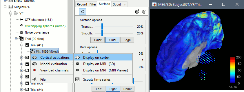
In the Scout tab, you can use the atlas "Source model" to display separately some regions difficult to observe with all the cortex. Typically the activity on the hippocampus surface. Click on the button [SEL] to display only the selected regions, then select the hippocampus entries. [TODO]
Compute statistics
We will now design a statistical analysis to assess the eyes-open and eyes-closed contrast. As a reminder, the recordings available in the database have already been filtered in the alpha frequency band (7-13Hz). As a measure of the global of the activity in this frequency band, we will average all the time samples in each block of 15s. Note that this is not the recommended procedure anymore: it would have been better to simply compute a PSD from the sources estimated for the continuous file link, but this option was not available at the time this tutorial was written.
In Process1, select all the subjects (except for Empty_Subject)and select [Process sources].
Run process Average > Average time > Use absolute value, All file.
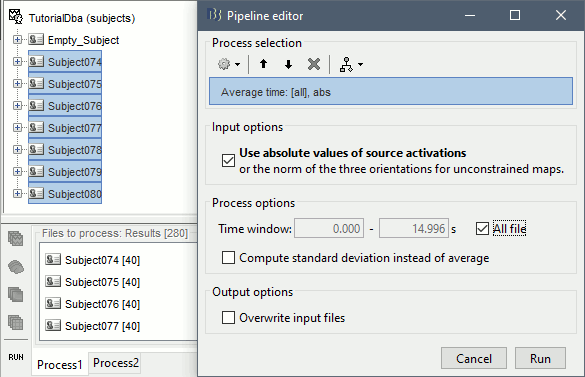
Then, the "Process2" tab is used : place the source power files of the eyes-closed condition in the "Files A" space and of the eyes-open condition in the "Files B" space.
To gain time, it is possible to sort the functional data by conditions, place the subjects in "FilesA" and "FilesB" and use the filter to include only files that contain 'avg' (for time-averaged files)Run a Student's T-Test to compute a statistical contrast between the conditions
![[ATTACH] [ATTACH]](/moin_static1911/brainstorm1/img/attach.png)
![[ATTACH] [ATTACH]](/moin_static1911/brainstorm1/img/attach.png)
The stat file can then be visualized and the values corresponding to subcortical structures are also appearing
![[ATTACH] [ATTACH]](/moin_static1911/brainstorm1/img/attach.png)
It is also interesting to observe the difference of means between conditions. To compute this, instead of runnning a Student's T-Test, select the "Difference of means" option
![[ATTACH] [ATTACH]](/moin_static1911/brainstorm1/img/attach.png)
Volume scouts
Some subcortical structures are modeled as volume source structures (for instance here, the thalamus and the amygdala). It is not possible to display scouts time series for these structures from the "Source model" or "Structures" atlases. It is necessary to create a new atlas, specific to volume scouts. The steps are the following :
- Second, to create a new scout :
Click on the "Create scout" cross, and click one point of the structure you want to include in the scout
Click on the "Increase scout size" as many times as necessary to include all the points of the volume, for example in the right thalamus
- Repeat this operation for all the volume scouts you want to create
References
Attal Y, Bhattacharjee M, Yelnik J, Cottereau B, Lefèvre J, Okada Y, Bardinet E, Chupin M, Baillet S (2009) Attal Y, Schwartz D (2013) Dumas T, Dubal S, Attal Y, Chupin M, Jouvent R (2013)
Modelling and detecting deep brain activity with MEG and EEG
IRBM, 30(3):133-138
Assessment of Subcortical Source Localization Using Deep Brain Activity Imaging Model with Minimum Norm Operators: A MEG Study
MEG Evidence for Dynamic Amygdala Modulations by Gaze and Facial Emotions
