|
Size: 5925
Comment:
|
Size: 7059
Comment:
|
| Deletions are marked like this. | Additions are marked like this. |
| Line 9: | Line 9: |
| This tutorial is based on resting-state recordings for 7 subjects with two conditions: eyes open (YO), eyes closed (YF). We have recorded 20 runs of 15 seconds for each subject and each condition, . | This tutorial is based on resting-state recordings for 7 subjects with two conditions: eyes open (YO), eyes closed (YF). We have recorded 20 runs of 15 seconds for each subject and each condition. |
| Line 13: | Line 13: |
| * Start by downloading the tutorial dataset: *file.zip*. * The file is an exported Brainstorm protocol. To load in your database, use the menu:<<BR>> File > Load Protocol > '''Load from zip file'''. <<BR>><<BR>> {{attachment:DBA_LoadProtocol.png||height="209",width="293"}} |
* Start by downloading the tutorial dataset '''TutorialDba.zip''' from the [[http://neuroimage.usc.edu/bst/download.php|Download]] page. * The file is an exported Brainstorm protocol. To load it in your database, use the menu:<<BR>> File > Load Protocol > '''Load from zip file'''. <<BR>><<BR>> {{attachment:loadzip.gif}} |
| Line 20: | Line 19: |
| * Double-click on "aseg atlas" (which contains the subcortical structures) | * Right-click on "aseg atlas" > '''Less vertices''' > '''15000''' vertices. <<BR>><<BR>> {{attachment:aseg_downsample.gif||height="213",width="436"}} * Double-click on "aseg atlas_15000V" (contains the subcortical structures from the FreeSurfer altas). |
| Line 22: | Line 22: |
| * Select the amygdala, the thalamus and the hippocampus, and create a subatlas | * Select the amygdala, the thalamus and the hippocampus, and create a subatlas. <<BR>><<BR>> {{attachment:aseg_keep.gif||height="385",width="555"}} |
| Line 24: | Line 24: |
| {{attachment:DBA_SelectStructures.png||height="353",width="444"}} | * '''Merge '''the cortex with the selected structures. '''Rename '''the new surface in "cortex_mixed". <<BR>><<BR>> {{attachment:aseg_merge.gif}} {{attachment:aseg_rename.gif}} |
| Line 26: | Line 26: |
| * Merge the cortex with the atlas of selected structures ; rename the structure created in CortexDBA | * Open the cortex_mixed surface and create a new atlas "'''Source model options'''". With Matlab 2015b+, the display looks weird because it limits the number of possible transparent layers to 5. To produce nicer figures, disable the OpenGL renderer (File > Edit preferences). The display will be much slower, but the renderer won't suffer from this limitation.<<BR>><<BR>> {{attachment:atlas_model.gif||height="214",width="668"}} |
| Line 28: | Line 28: |
| {{attachment:DBA_MergeSurfaces.png||height="295",width="223"}} {{attachment:DBA_RenameCtx.png||height="198",width="135"}} | * Set the set modeling options to "'''Deep brain'''" for all the structures.<<BR>><<BR>> {{attachment:atlas_dba.gif||height="246",width="606"}} |
| Line 30: | Line 30: |
| * Create a new atlas "Source Model Atlas", and set modeling options to "Deep brain" | == Source estimation == ==== Head model ==== * In Process1, select all the subject folders. Click on [Process recordings]. * Run process '''Sources > Compute head model''': Custom source model, MEG=Overlappling spheres. <<BR>><<BR>> {{attachment:dba_headmodel.gif||height="379",width="405"}} |
| Line 32: | Line 35: |
| {{attachment:DBA_SourceModelOptions.png||height="193",width="437"}} {{attachment:DBA_SetModelingOptions.png||height="213",width="440"}} == Compute source activity == Then, compute a headmodel for each subject as "Custom Source Model" ; it is advised to run it as batch from the pipeline editor. {{attachment:DBA_HeadModelBatch.png}} {{attachment:DBA_HeadModelOptions.png}} |
==== Inverse model ==== |
| Line 43: | Line 38: |
| {{attachment:DBA_ComputeSources.png}} {{attachment:DBA_SourceOptions.png}} {{attachment:DBA_SourceOptions2.png}} | {{attachment:DBA_ComputeSources.png||height="244",width="171"}} {{attachment:DBA_SourceOptions.png||height="232",width="156"}} {{attachment:DBA_SourceOptions2.png||height="289",width="143"}} |
| Line 47: | Line 42: |
| {{attachment:DBA_VisuActivity.png}} | {{attachment:DBA_VisuActivity.png||height="351",width="478"}} |
| Line 49: | Line 44: |
| If the activity of the volume structures (thalamus and amygdala here) do not appear, try moving the Min size cursor to max and then back to 1. | If activities of the volume structures (thalamus and amygdala here) do not appear, try moving the Min size cursor to max and then back to 1. |
| Line 54: | Line 49: |
| * First, the alpha-power is time-averaged for each run<<BR>> {{attachment:DBA_AverageTime.png}} {{attachment:DBA_AverageTimeOptions.png}} | * First, the alpha-power is time-averaged for each run<<BR>><<BR>> {{attachment:DBA_AverageTime.png||height="259",width="303"}} {{attachment:DBA_AverageTimeOptions.png||height="216",width="236"}} |
| Line 57: | Line 52: |
| * Run a Student's T-Test to compute a statistical contrast between the conditions<<BR>> {{attachment:DBA_Ttest.png}} {{attachment:DBA_TtestOptions.png}} * The stat file can then be visualized and the values corresponding to subcortical structures are also appearing<<BR>> {{attachment:DBA_VisuStat.png}} * It is also interesting to observe the difference of means between conditions. To compute this, instead of runnning a Student's T-Test, select the "Difference of means" option<<BR>> {{attachment:DBA_DiffOfMeans.png}} |
* Run a Student's T-Test to compute a statistical contrast between the conditions<<BR>><<BR>> {{attachment:DBA_Ttest.png||height="422",width="383"}} {{attachment:DBA_TtestOptions.png||height="283",width="226"}} * The stat file can then be visualized and the values corresponding to subcortical structures are also appearing<<BR>><<BR>> {{attachment:DBA_VisuStat.png||height="286",width="523"}} * It is also interesting to observe the difference of means between conditions. To compute this, instead of runnning a Student's T-Test, select the "Difference of means" option<<BR>><<BR>> {{attachment:DBA_DiffOfMeans.png||height="283",width="394"}} |
| Line 62: | Line 57: |
| Some subcortical structures are modeled as volume source structures (for instance here, the thalamus and the amygdala). It is not possible to display scouts time series for these structures from the "Source model" or "Structures" atlases. It is necessary to create a new atlas, specific to volumic scouts. The steps are the following : | Some subcortical structures are modeled as volume source structures (for instance here, the thalamus and the amygdala). It is not possible to display scouts time series for these structures from the "Source model" or "Structures" atlases. It is necessary to create a new atlas, specific to volume scouts. The steps are the following : |
| Line 64: | Line 59: |
| * First, create the volumic atlas<<BR>> {{attachment:DBA_VolumeScouts.png}} | * First, create the volume atlas<<BR>><<BR>> {{attachment:DBA_VolumeScouts.png||height="264",width="668"}} |
| Line 66: | Line 62: |
| * Click on the "Create scout" cross, and click one point of the structure you want to include in the scout<<BR>> {{attachment:DBA_VolumeScout_FirstPoint.png}} * Click on the "Increase scout size" as many times as necessary to include all the points of the volume, for example in the right thalamus<<BR>> {{attachment:DBA_IncreaseScoutSize.png}} {{attachment:DBA_Scout_RightThal.png}} * Rename the scout and set the correct region and the desired function<<BR>> {{attachment:DBA_RenameScout.png}} {{attachment:DBA_SetRegion.png}} {{attachment:DBA_SetFunction.png}} * Repeat this operation for all the volumic scouts you want to create * Finally, you can display time series of your choice<<BR>> {{attachment:DBA_DispolayScoutsTS.png}} |
* Click on the "Create scout" cross, and click one point of the structure you want to include in the scout<<BR>> {{attachment:DBA_VolumeScout_FirstPoint.png||height="291",width="659"}} * Click on the "Increase scout size" as many times as necessary to include all the points of the volume, for example in the right thalamus<<BR>> {{attachment:DBA_IncreaseScoutSize2.png||height="239",width="148"}} {{attachment:DBA_Scout_RightThal.png||height="272",width="266"}} * Rename the scout and set the correct region and the desired function<<BR>><<BR>> {{attachment:DBA_RenameScout.png||height="78",width="192"}} {{attachment:DBA_SetRegion2.png||height="271",width="260"}} {{attachment:DBA_SetFunction2.png||height="270",width="244"}} * Repeat this operation for all the volume scouts you want to create * Finally, you can display time series of your choice<<BR>><<BR>> {{attachment:DBA_DispolayScoutsTS.png||height="306",width="280"}} |
| Line 76: | Line 75: |
| Attal Y, Bhattacharjee M, Yelnik J, Cottereau B, Lefèvre J, Okada Y, Bardinet E, Chupin M, Baillet S (2009)<<BR>>[[http://www.ncbi.nlm.nih.gov/pubmed/18003114|Modelling and detecting deep brain activity with MEG and EEG]]<<BR>> . '''IRBM''', 30(3):133-138 |
Attal Y, Bhattacharjee M, Yelnik J, Cottereau B, Lefèvre J, Okada Y, Bardinet E, Chupin M, Baillet S (2009)<<BR>>[[http://www.ncbi.nlm.nih.gov/pubmed/18003114|Modelling and detecting deep brain activity with MEG and EEG]]<<BR>>'''IRBM''', 30(3):133-138 |
DBA tutorial: Compute sources in deep cerebral structures
Authors: Jean-Eudes Le Douget, Francois Tadel, Denis Schwartz
This tutorial explains step-by-step how to use the DBA (Deep Brain Activity) functionality, useful to assess subcortical source localization.
Contents
Import database
This tutorial is based on resting-state recordings for 7 subjects with two conditions: eyes open (YO), eyes closed (YF). We have recorded 20 runs of 15 seconds for each subject and each condition.
The goal is to compute the contrast between the two conditions in the alpha band. The data has already been filtered in the alpha frequency band (7-13Hz) and the default anatomy is used for all the subjects.
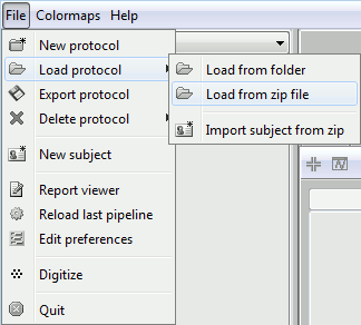
Start by downloading the tutorial dataset TutorialDba.zip from the Download page.
The file is an exported Brainstorm protocol. To load it in your database, use the menu:
File > Load Protocol > Load from zip file.
Select deep structures
The first step consists in creating the surface file that includes the cortex and the deep structures that we want to include in the model. Here, in the default anatomy:
Right-click on "aseg atlas" > Less vertices > 15000 vertices.
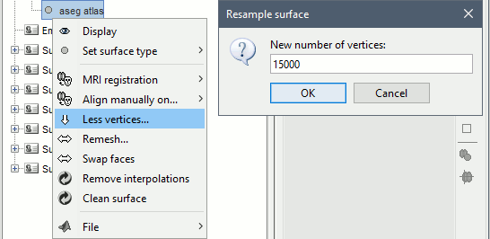
Double-click on "aseg atlas_15000V" (contains the subcortical structures from the FreeSurfer altas).
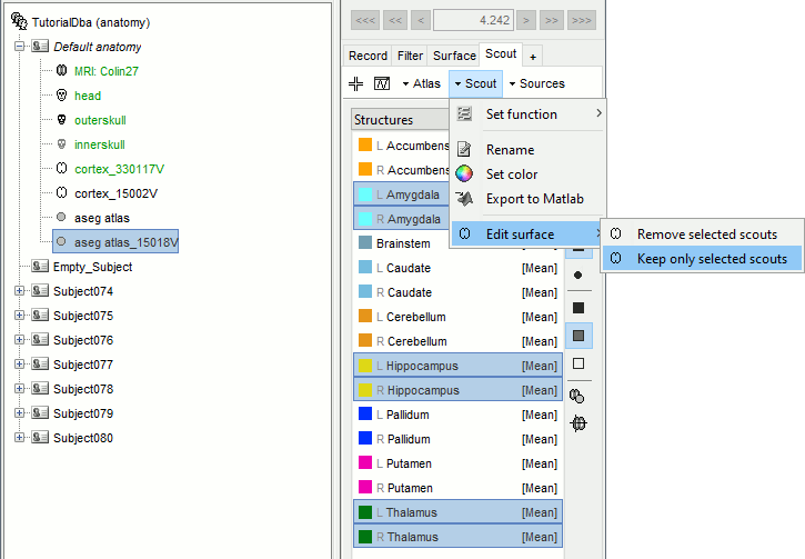
Select the amygdala, the thalamus and the hippocampus, and create a subatlas.
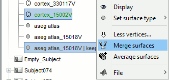
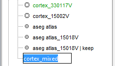
Merge the cortex with the selected structures. Rename the new surface in "cortex_mixed".
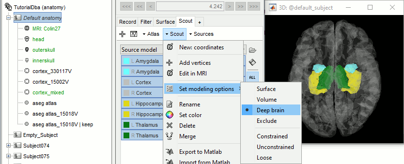
Open the cortex_mixed surface and create a new atlas "Source model options". With Matlab 2015b+, the display looks weird because it limits the number of possible transparent layers to 5. To produce nicer figures, disable the OpenGL renderer (File > Edit preferences). The display will be much slower, but the renderer won't suffer from this limitation.

Set the set modeling options to "Deep brain" for all the structures.
Source estimation
Head model
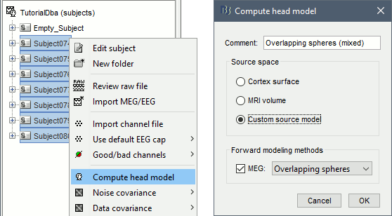
- In Process1, select all the subject folders. Click on [Process recordings].
Run process Sources > Compute head model: Custom source model, MEG=Overlappling spheres.
Inverse model
At this stage, it is now possible to compute sources.
You can now visualize activity the same way as for usual headmodels.
If activities of the volume structures (thalamus and amygdala here) do not appear, try moving the Min size cursor to max and then back to 1.
Compute statistics
Now that the source calculations are done, we design a statistical analysis to assess the eyes-open and eyes-closed contrast.
Then, the "Process2" tab is used : place the source power files of the eyes-closed condition in the "Files A" space and of the eyes-open condition in the "Files B" space.
To gain time, it is possible to sort the functional data by conditions, place the subjects in "FilesA" and "FilesB" and use the filter to include only files that contain 'avg' (for time-averaged files)Run a Student's T-Test to compute a statistical contrast between the conditions
![[ATTACH] [ATTACH]](/moin_static1911/brainstorm1/img/attach.png)
![[ATTACH] [ATTACH]](/moin_static1911/brainstorm1/img/attach.png)
The stat file can then be visualized and the values corresponding to subcortical structures are also appearing
![[ATTACH] [ATTACH]](/moin_static1911/brainstorm1/img/attach.png)
It is also interesting to observe the difference of means between conditions. To compute this, instead of runnning a Student's T-Test, select the "Difference of means" option
![[ATTACH] [ATTACH]](/moin_static1911/brainstorm1/img/attach.png)
Volume scouts
Some subcortical structures are modeled as volume source structures (for instance here, the thalamus and the amygdala). It is not possible to display scouts time series for these structures from the "Source model" or "Structures" atlases. It is necessary to create a new atlas, specific to volume scouts. The steps are the following :
- Second, to create a new scout :
Click on the "Create scout" cross, and click one point of the structure you want to include in the scout
Click on the "Increase scout size" as many times as necessary to include all the points of the volume, for example in the right thalamus
- Repeat this operation for all the volume scouts you want to create
DBA constraints [TODO]
Describe the constraints applied to each region.
References
Attal Y, Bhattacharjee M, Yelnik J, Cottereau B, Lefèvre J, Okada Y, Bardinet E, Chupin M, Baillet S (2009)
Modelling and detecting deep brain activity with MEG and EEG
IRBM, 30(3):133-138
Attal Y, Schwartz D (2013)
Assessment of Subcortical Source Localization Using Deep Brain Activity Imaging Model with Minimum Norm Operators: A MEG Study
PLOS ONE, 8(3):e59856
Dumas T, Dubal S, Attal Y, Chupin M, Jouvent R (2013)
MEG Evidence for Dynamic Amygdala Modulations by Gaze and Facial Emotions
PLOS ONE, 8(9): e74145
