|
Size: 45614
Comment:
|
Size: 37353
Comment:
|
| Deletions are marked like this. | Additions are marked like this. |
| Line 1: | Line 1: |
| NIRSTORM '''Author: ''Thomas Vincent, PERFORM Centre and physics dpt., Concordia University, Montreal, Canada'' <<BR>> (thomas.vincent at concordia dot ca)''' '''Collaborators:''' * '''''Zhengchen Cai, PERFORM Centre and physics dpt., Concordia University, Montreal, Canada'' ''' * '''''Alexis Machado, Multimodal Functional Imaging Lab., Biomedical Engineering Dpt, McGill University, Montreal, Canada'' ''' * '''''Louis Bherer, Centre de recherche, Institut de Cardiologie de Montréal, Montréal, Canada'' ''' * '''''Jean-Marc Lina, Electrical Engineering Dpt, Ecole de Technologie Supérieure, Montréal, Canada'' ''' * '''''Christophe Grova, PERFORM Centre and physics dpt., Concordia University, Montreal, Canada''''' * '''''Edouard Delaire, Physics Department and PERFORM Center, Concordia University, Montreal, Canada''''' * '''''Thomas Vincent, EPIC center, Montreal Heart Institute, Montreal, Canada''''' '''The tools mentioned are an integral part of Nirstorm, a brainstorming plugin specialized in the analysis of NIRS data, also known as functional near-infrared spectroscopy (fNIRS). It provides dedicated tools for data pre-processing, visualization, analysis and modeling.''' '''This tutorial offers three separate tutorials: Channel-space analysis,Source-space analysis: reconstruction of the motor response on the cortical surface and Optimal Montage. @Edouard''' ''' ''' fNIRS: Channel-space analysis This tutorial demonstrates the process of estimating the sensor-level response of near-infrared spectroscopy (fNIRS) to a finger-tapping task. It also covers the statistical analysis using a general linear model (GLM) at the subject level. Below is a handy reference sheet highlighting the key features of Brainstorm that will be utilized throughout the tutorials: The tools presented here are part of nirstorm, which is a brainstorm plug-in dedicated to fNIRS (also known as functional near-infrared spectroscopy fNIRS) data analysis. This current tutorial only illustrates basic features on how to import and process fNIRS recordings in Brainstorm. To go further, please visit the [[https://github.com/Nirstorm/nirstorm/wiki|nirstorm wiki]]. There you can find the [[https://github.com/Nirstorm/nirstorm/wiki/Workshop-PERFORM-Week-2018|latest set of tutorials]] covering optimal montage and source reconstruction, that were given at the last PERFORM conference in Montreal (2022). Setup click on the link to access the installation procedures for Nirstorm: https://github.com/Nirstorm/nirstorm/wiki/Installation '''Requirements''': You have already completed all introductory tutorials #1-#7and have a working copy of Brainstorm installed on your computer. Subject importation To make sure we all have the same dataset, we have prepared a subject with the imported anatomy.To import this subject in Brainstorm, click on'' File'' >'' load protoco''l > ''import subject from zip'' and then select T''utorialNIRSTORM_Subject01.zip'' under the bst_db folder. For the rest of the tutorial, ensure that the remeshed head and the mid-cortical surface are chosen as the default surface. You can identify them by their green appearance, as shown in the picture below. Your Brainstorm database should resemble the example depicted in the picture: {{blob:https://neuroimage.usc.edu/bc753881-f621-4e77-83c6-2b39cad04c4d|pastedGraphic.png}} {{blob:https://neuroimage.usc.edu/d6aa827f-3277-429f-a67c-d00726f2ff8a|pastedGraphic_1.png}} Import fNIRS functional data The functional data used in this tutorial comes from the Brainsight acquisition software and can be found in the Functional folder. It consists of the following files: * '''fiducials.txt''': This file contains the coordinates of fiducial points (nasion, left ear, right ear). These points have been digitized at the same locations as the fiducials marked on the anatomical MRI. Brainstorm will use these points for registration, so it's important that the digitized and marked fiducials are consistent for accurate results. * '''optodes.txt:''' This file contains the coordinates of the optodes, which include sources and detectors. The coordinates are in the same reference system as fiducials.txt. Note that the specific reference system is not significant here since Brainstorm will perform the registration later. * '''tapping.nirs''': This file contains fNIRS (near-infrared spectroscopy) data in a Homer-based format. Please note that the "SrcPos" and "DetPos" fields in the file will be updated to match the provided coordinates in "optodes.txt". '''=>Mettre à jour optodes.txt @Edouard''' |
= NIRSTORM: a Brainstorm extension dedicated to functional Near Infrared Spectroscopy (fNIRS) data analysis, advanced 3D reconstructions, and optimal probe design. = Authors: Édouard Delaire, Dr. Christophe Grova This tutorial aims to introduce NIRSTORM. NISTORM is a plug-in dedicated to the analysis of functional near-infrared spectroscopy (fNIRS) data inside the Brainstorm software. This tutorial covers three main features of the NIRSTORM package: (1) Data importation and preprocessing (2) Data analysis at the channel level (3) Data analysis on the cortex after 3D reconstruction. This tutorial assumes that you are already familiar with the Brainstorm environment. If this is not the case, we recommend following Brainstorm tutorials 1 to 7. <<TableOfContents(2,2)>> == Introduction == === Presentation of the experiment === The acquisition protocol and the general workflow presented in this tutorial from fNIRS optimal montage design to 3D reconstruction is described in further detail in Cai et al, 20211. We are considering fNIRS data acquired on one healthy subject, featuring one run of 19 minutes acquired with a sampling rate of 10Hz on a CW fNIRS Brainsight device (Rogue-Research Inc., Montreal, Canada) * Finger tapping task of the left hand: 20 blocks of 10 seconds of finger tapping task each, with a rest period of 30 to 60 seconds. * Personalized optimal montage targeting the right motor knob, featuring 3 dual wavelength sources, 15 detectors, and 1 proximity detector. 2 wavelengths: 685nm and 830nm * 3T high-resolution anatomical MRI data processed using FreeSurfer 5.3.0. (https://surfer.nmr.mgh.harvard.edu) === Setup === {{attachment:img1.png||width="50%"}} Using the Brainstorm plug-in system, download the following plugins : * NIRS > NIRSTORM : the core of NIRSTORM package * NIRS > MCXLAB-cl : a plugin for the estimation of the fNIRS forward model using Monte Carlo simulations of infrared light photons in the anatomical head model * Inverse > Brainentropy: our package dedicated to solving the fNIRS reconstruction inverse problem using the Maximum Entropy on the Mean framework === Downloading the dataset. === The total disk space required after data download and installation is ~1.3Go. The size is quite large because of the optical data that are required for the computation of the forward model. The dataset can be downloaded from: https://osf.io/md54y/?view_only=0d8ad17d1e1449b5ad36864eeb3424ed . '''License:''' This tutorial dataset (fNIRS and MRI data) remains proprietary of the MultiFunkIm Laboratory of Dr Grova, at Concordia School of Health, Concordia University, Montreal. Its use and transfer outside the Brainstorm tutorial, e.g. for research purposes, is prohibited without written consent from our group. For questions please contact Dr. Christophe Grova: christophe.grova@concordia.ca == Data importation and preprocessing == Description of the data organization The data are organized using the following scheme according to BIDS standards: {{attachment:img2.png||width="100%"}} === Data Importation === * Start Brainstorm (Matlab scripts or stand-alone version) * Select the menu File > Create new protocol. Name it "TutorialNIRS" and select the options: "No, use individual anatomy", "No, use one channel file per acquisition run (MEG/EEG)". In terms of sensor configuration, fNIRS is similar to EEG and the placement of optodes may be subject-specific. Also, the channel definition will change during data processing, this is the reason why you should always use one channel file per acquisition run, even if the optode placement remains the same. === Importing anatomical data === Import anatomical data Following tutorials 1-2, import the subject anatomy segmented using freesurfer using the following fiducials coordinate in MRI coordinate: Switch to the "anatomy" view of the protocol. * Right-click on the TutorialNIRS folder > New subject > sub-01 * Leave the default options you set for the protocol * Right-click on the subject node > Import anatomy folder: * Set the file format: "Freesurfer + volumes atlases" * Select the folder: nirstorm_tutorial_2024/derivatives/FreeSurfer/sub-01 * Number of vertices of the cortex surface: 15000 (default value) * Answer "yes" when asked to apply the transformation. * Set the 3 required fiducial points, indicated below in (x,y,z) MRI coordinates. * You can right-click on the MRI viewer > Edit fiducial positions > MRI coordinates, and copy-paste the following coordinates in the corresponding fields. Click [Save] when done. * Nas : [ 131, 213, 117 ] * Lpa : [ 51, 116, 80 ] * Rpa : [ 208, 117, 86 ] * Ac : [ 131, 128, 130 ] * Pc : [ 129, 103, 124 ] * Ih : [ 133, 135, 176 ] * Once the anatomy is imported, make sure that the surface "mid_15002V" is selected (green). If it is not, right-click on it and select "set as default cortex". This will define the cortical surface on which fNIRS 3D reconstructions will be estimated. * Resample the head mask to get a uniform mesh on the head. For that, right-click on the head mask and select remesh, then 10242 vertices. This allows us to get a uniform mesh on the head. Your database should look like this: {{attachment:img3.png||width="70%"}} Note that the elements that appear in green correspond to those used for later computations. It is important that the new head mask (remeshed) and the mid-surface (mid_15002V) are selected and appear green in your database. Additionally, we defined the hand knob on the mid-surface. Open the mid surface, and use Atlas > Add scouts to Atlas and select the FreeSurfer annotation: NIRSTORM-data/derivatives/segmentation/sub-01/scout_hand.annot === Import fNIRS functional data === The Brainsight acquisition software produced the functional fNIRS data used in this tutorial and is available in the data subfolder of the fNIRS sample folder(nirstorm_tutorial_2024/sub-01/nirs). The data were exported according to the BIDS format: See https://bids-specification.readthedocs.io/en/stable/modality-specific-files/near-infrared-spectroscopy.html for a description of each file. |
| Line 58: | Line 91: |
| * Right-click on Subject 01 > '''Review raw file * Select file type '''NIRS: Brainsight (.nirs) * Select file tapping.nirs.Note: the importation process assumes that the files optodes.txt and fiducials.txt are in the same folder as the .nirs data file. We obtain the following image: {{blob:https://neuroimage.usc.edu/e1d09c6d-dff5-4c8d-ae23-3dfccf765d5d|pastedGraphic_2.png}} Registration Similar to the tutorial on MEG-MRI coregistration(https://neuroimage.usc.edu/brainstorm/Tutorials/ChannelFile), the registration process between the MRI and fNIRS data in this tutorial also begins with three reference points: Nasion, Left ear, and Right ear. This initial registration can be further refined using either the complete shape of the subject's head or through manual adjustment. The initial registration relies on three fiducial points that establish the Subject Coordinate System (SCS): Nasion, Left ear, and Right ear. Before acquiring the fNIRS recordings, these same three points were marked. The person conducting the subject's recording used a tracking device (in this case, Brainsight) to digitize and save the positions of these points in the fNIRS datasets (refer to fiducials.txt). When the fNIRS recordings are loaded into the Brainstorm database, they are aligned with the MRI using these fiducial points. The NAS/LPA/RPA points digitized with Brainsight are matched with the corresponding points we placed in the MRI Viewer. To enhance the accuracy of this registration, we strongly recommend users to digitize additional points on the subject's head. Ideally, around 100 points should be uniformly distributed on the rigid parts of the head, such as the skull (from nasion to inion), eyebrows, ear contour, and nose crest. It is important to avoid marking points on the softer parts of the head (such as cheeks or neck) since their shape may differ when the subject is seated or lying down in the MRI. For more detailed information on digitizing head points, please refer to the provided resource. To import the head points: * right-click on NIRS-BRS channels (104) * select Edit * Then select the file called head points in the Functional folder with the format EEG: ASCII, name,XYZ(.). * Right click on NIRS-BRS channels (104) and select Digitalized head points > Remove points below nasion, * finally Right click on NIRS-BRS channels (104) and select `MRI registration > Refine using head points (ignore 0% of the headpoints) We obtain the following image: {{blob:https://neuroimage.usc.edu/6d8f5544-07fe-4204-8c4a-57cfa6aece3b|pastedGraphic_3.png}} To verify our result, it is interesting to check the distance between 167 head points and head Surface. {{blob:https://neuroimage.usc.edu/15231472-71e3-4640-91a4-44988ad2cf72|pastedGraphic_4.png}} Visualize fNIRS signals To visualize fNIRS signals: * Right-click on ''Link to raw file '' * Under the tapping condition and use'' NIRS>Display time series.'' It will open a new figure with superimposed channels. we obtain the following curves : Note that it is advisable to set the coordinate axis to Flipe Y (by default, the software sets the values on the axis in reverse). Exact Stimulation events: During the experiment, the stimulation paradigm was executed using E-Prime, which sent triggers to the acquisition device through the parallel port. These stimulation events are then stored as a boxcar signal in the AUX1 channel: values above a certain threshold indicate a stimulation block. To view the auxiliary data: * Right-click on Link to raw file * Select NIRS_AUX > Display time series In the event panel: * Click on file * Read events from channel and use the following options: we obtain the following diagram: The default time window can be limited to a few seconds. To view the complete time series: * in the main brainstorm window -- right panel * go to the "Record" tab, * change "Start" to 0 and "Duration:" to 709.3s (you can see the total duration at the top right of the brainstorm main window). Indeed, Brainstorm uses a dynamic montage called "NIRS Overlay" to group and color-code NIRS time series based on wavelength (red: 830nm, green: 686nm). When using the selection tool, the signals for a given pair of sources and detectors are also grouped. Therefore, by clicking on a curve for one wavelength, you will also select the other wavelength for the same pair. To isolate the signals from a selected pair, you can use the default behavior of Brainstorm by pressing ENTER or right-clicking on the figure and selecting "Channel > View selected". However, please note that the dynamic fNIRS overlay montage is not activated in this case. Pre-processing The Pre-processing of data in fNIRS software offers the possibility of improving measurement quality, performing advanced analyses and standardizing analysis procedures, all of which contribute to a better interpretation and understanding of fNIRS data. To add the "Link to raw" file to the processing box, simply drag and drop it onto the box. Once it's in place, click on the "Run" button to execute the process. You can create a pipeline by sequentially adding additional processes to the existing ones. Add the following process to your pipeline * ''NIRS > Pre-process > Detect Bad channels'' '''@Edouard''' '''The beauty of the "Detect Bad Channels" function lies in its ability to identify and report faulty channels in the data, improving the quality and reliability of the results obtained during data analysis.To detect faulty channels, the software uses a variety of methods, including outlier detection, inter-channel coherence and variance analysis, spatial feature analysis and visual inspection. In this example, a coefficient of variation of 8% has been used. If channels exceed this threshold, they are considered to be potentially faulty and present artifacts. By removing auxiliary measurements, these channels can be excluded from further analysis, ensuring more accurate interpretation of the data.''' * ''NIRS > dOD and MBLL > raw to delta OD'' '''@Edouard''' '''The purpose of the "NIRS > dOD and MBLL > raw to delta OD" function is to perform a specific transformation on NIRS data. This transformation consists in converting the raw data into variations in cerebral oxygenation (delta OD) using the diffusion-based correction approach (MBLL - Modified Beer-Lambert Law). The appeal of this feature lies in its ability to extract variations and reduce artifacts from NIRS data.''' '''In this example, the "mean" baseline method was used to adjust the data by subtracting a value representing background activity. In addition, filling was applied to replace missing or corrupted data with estimated values.''' * ''Pre-process > Band-pass filter'' '''@Edouard''' '''The advantage of the "Pre-process > Band-pass filter" function in Brainstorm software lies in its ability to apply a band-pass filter to NIRS data. This feature highlights frequency bands of interest by applying a bandpass filter to the data.''' '''When using the bandpass filter function in Brainstorm software, you can specify different parameters to filter NIRS data. Here's an explanation of the parameters mentioned:''' '''-Sensor types or name: This option lets you select the specific sensors you wish to filter. You can choose to apply the filter to all sensors or only to a subset of sensors based on their types or names.''' '''-Lower cut frequency: This is the filter's lower cutoff frequency. ''' '''-Upper frequency: This is the filter's upper cutoff frequency. ''' '''-Transition: This refers to the width of the transition band between the filter pass zone and the filter stop zone.''' '''-Stop band: This indicates the maximum attenuation (in decibels) in the filter stop band. In other words, frequencies outside the stop band will be attenuated by at least 40 dB.''' '''Filter version 2019: This is the version of the filter used in Brainstorm. ''' * ''NIRS > Pre-process > Remove superficial noise'' '''@Edouard''' '''The "NIRS > Pre-process > Remove superficial noise" function in the Brainstorm software eliminates unwanted superficial noise from NIRS data, improving the quality, specificity and reliability of the brain measurements obtained.To achieve this, the software selects specific channels for processing, models surface noise and subtracts it from the NIRS data.''' '''Here is an explanation of the parameters mentioned:''' '''-Short-separation channels based on Source-detector distances: This option uses short-separation channels based on source-detector distances. In NIRS systems, short-separation channels are designed to measure primarily the signal from superficial tissues, such as the scalp.''' '''-Separation threshold of 1.5 cm: This separation threshold is used to identify short separation channels. Channels with a distance between source and detector of less than 1.5 cm are considered short separation channels.''' '''-Baseline from 0 to 1123.2 s: This option specifies the time period to be used to calculate the baseline. The baseline is then subtracted from the data to eliminate slow and stationary variations.''' * ''NIRS > dOD and MBLL > MBLL delta OD to delta [HbO], [HbR] & [HbT]'' '''@Edouard''' '''The "NIRS > dOD and MBLL > MBLL delta OD to delta [HbO], [HbR] & [HbT]" function in Brainstorm software converts estimated variations in cerebral oxygenation into specific variations in oxygenated, deoxygenated and total hemoglobin.To perform this conversion, Brainstorm software calibrates and estimates the parameters, applies the Beer-Lambert equation, and corrects for artifacts and biases. Process parameters : -Age: subject's age, used to correct partial light path length. -Basic method: mean or median. Method for calculating reference intensity (I_ref) against which to calculate variations -PVF: partial volume factor. -Light path correction: flag to actually correct light diffusion. If unchecked, dpf/pvf is set to 1. ''' Then click on Run. The following report should appear : {{blob:https://neuroimage.usc.edu/0ab89bb8-0486-41ea-8ca9-a0c808ab5055|pastedGraphic_5.png}} Window averaging The objective is to analyze the response produced by the motor paradigm. To achieve this, we apply a technique called window-averaging, which focuses on specific time intervals centered around each motor onset. This approach helps account for any baseline variations observed across trials. The initial step involves dividing the data into segments that align with the desired window for averaging. The width of the average window exceeds that of the stimulation events. This broader window allows us to observe the return to baseline or the undershoot that occurs after the stimulation period. Please ensure that the "Use events" option is checked and that the tapping events are selected. The reference time should range from -10000 ms to 30000 ms (-10000 ms to 30000 ms). This means there will be 10 seconds before the stimulation event to check for signal stability, and 30 seconds after stimulation to observe the return to baseline or undershoot. ''' '''⚠️In the "Pre-processing" panel, check the "Remove DC offset" option and use a time range from -10000 ms to 0 ms. This will set a reference window before removing any offset from the segments. All signals will be centered around zero based on this window.''' '''Lastly, ensure that the "Create a separate folder for each event type" option is unchecked. * Right-click on "'''Link to raw file | band(0.01-0.1Hz)| SSC (mean)''': [0.000s,1123.200s] » * under the condition "tapping_dOD_Hb" * use Import in database using the following parameter : This will create 20''' listening files''', each corresponding to an individual trial, which you can examine separately. Any trial with excessive movement can be rejected by right-clicking on it and selecting the "Reject trial" option. In our example, we want to reject the first trial as it is contaminated by the transient_bandpass filter effect. To calculate the average response, drag and drop the 20 files into the processing box, which will display "tapping (20 files) [19]". The number 19 indicates that only 19 out of the 20 files will be used (since we rejected 1 trial). You can then visualize the average by inspecting the AvgStderr file: "tapping (19)". * Click on ''run'' * select the process ''Average '' * Average files * Use the function ''Arithmetic average + Standard error '' * use the option Keep all event markers from the individual epochs. The following report should appear : '''@Edouard''' {{blob:https://neuroimage.usc.edu/3475bbdb-4f32-420f-8c72-985ad6df5fa2|pastedGraphic_6.png}} We obtain the following images: (we've added a topographic view (right-click>View topography)) In addition, for a complete analysis we can use the 2D layout (NIRS>2D Layout). This function provides a representation of a « time countdown ». '''@Edouard''' ⚠️''' It's important to note that the data are in seconds rather than milliseconds. This is due to the nature of EEG data, where values are generally recorded and processed in seconds. ''' General Linear Model the use of the General Linear Model (GLM) in Brainstorm software for fNIRS data enables advanced statistical analysis, covariate control, artifact correction, brain activation estimation and cross-validation analysis. This contributes to an in-depth understanding of fNIRS data and the identification of relationships between fNIRS measurements and factors of interest. Please note that the short channel regression should not be performed twice. If you are using the GLM (Generalized Linear Model), we recommend performing the short channel regression within the GLM module. To create the following pipeline, drag and drop the "Link to raw file | band(0.01-0.1Hz)" from the tapping_dOD condition: '''A Expliquer ''' '''>Mentionner analyse de groupe ??? @Edouard''' * NIRS > dOD and MBLL > MBLL delta OD to delta [HbO], [HbR] & [HbT] '''@Edouard''' '''The "NIRS > dOD and MBLL > MBLL delta OD to delta [HbO], [HbR] & [HbT]" function in Brainstorm software converts estimated variations in cerebral oxygenation into specific variations in oxygenated, deoxygenated and total hemoglobin.To perform this conversion, Brainstorm software calibrates and estimates the parameters, applies the Beer-Lambert equation, and corrects for artifacts and biases. Process parameters : -Age: subject's age, used to correct partial light path length. -Basic method: mean or median. Method for calculating reference intensity (I_ref) against which to calculate variations -PVF: partial volume factor. -Light path correction: flag to actually correct light diffusion. If unchecked, dpf/pvf is set to 1.''' * NIRS > GLM > 1st level design and fit '''@Edouard''' '''the "NIRS > GLM > 1st level design and fit" step refers to the application of a generalized linear model (GLM) to fit NIRS data to a specific experimental design model.''' '''The GLM is used to model the relationship between brain activity measurements and experimental parameters, such as experimental conditions, events or stimuli.''' '''When you perform the "1st level design and fit" step in Brainstorm software, you can specify various parameters, such as FIR filtering, HRF model, short separation channel detection, and pre-coloring method. ''' '''-FIR (Finite Impulse Response) filtering: FIR filtering is used to attenuate unwanted low-frequency components in NIRS data. The "high pass filter" parameter lets you specify the low cutoff frequency, i.e. the frequency below which low-frequency components will be attenuated. For example, if you specify 0.01 Hz as the low cutoff frequency, all frequencies below 0.01 Hz will be attenuated.''' '''-High pass filter frequency: This parameter determines the high pass frequency of the FIR filter. This is the frequency at which high-frequency components are attenuated.''' '''Transition band: This parameter defines the width of the transition band between the filter pass zone and the FIR filter stop zone.''' '''Minimum period for stimulation event : This parameter specifies the minimum period required between two stimulation events for them to be considered as separate events. For example, if you specify 200 seconds as the minimum period, any stimulation event occurring less than 200 seconds after a previous event will be considered a continuation of that previous event.''' '''-HRF (Hemodynamic Response Function) model: The HRF model is used to represent the hemodynamic response in the brain in response to a stimulation or event. The "HRF model" parameter is used to specify the model used to model this response. ''' '''short separation channels based on source-detector distances) : This parameter detects short separation channels based on source-detector distances. Channels whose distance is less than the specified threshold (1.5 in the example) are considered short separation channels.''' '''-Pre-coloring method: The pre-coloring method is used to compensate for systematic variations or differences in sensitivity between short separation channels and other channels. This method improves measurement quality by correcting potential biases.''' '''In summary, during the "1st level design and fit" step in Brainstorm, you can specify various parameters such as FIR filtering, HRF model, short separation channel detection and pre-coloring method. These parameters are used to pre-process NIRS data, model the hemodynamic response, detect short separation channels and compensate for potential biases in order to obtain more accurate and reliable analysis results.''' * NIRS > GLM > 1st level contrast '''@Edouard''' '''the "NIRS > GLM > 1st level contrast" step in Brainstorm allows you to specify the contrasts of interest and perform statistical analyses to test for differences in brain response between experimental conditions or groups within the GLM model. This makes it possible to identify specific brain activations associated with explanatory variables, or to highlight significant differences between the conditions or groups studied.''' * NIRS > GLM > contrast t-test '''@Edouard''' '''The "NIRS > GLM > contrast t-test" step in Brainstorm is used to perform t-tests to assess the statistical significance of the contrasts specified in the GLM model applied to the NIRS data. This determines whether observed differences between experimental conditions or groups are statistically significant, and provides a sound statistical basis for interpreting the results of NIRS data analysis.''' '''A one-tailed contrast test is used when you want to test a directional hypothesis, i.e. you expect a positive or negative difference between conditions or groups. En revanche, un test de contraste bilatéral est utilisé lorsque l'on souhaite tester une hypothèse non directionnelle, c'est-à-dire que l'on s'attend simplement à une différence entre les conditions ou les groupes, sans spécifier une direction particulière.''' We obtain the following images: fNIRS: Source-space analysis: reconstruction of the motor response on the cortical surface This tutorial demonstrates the process of estimating the sensor-level response of near-infrared spectroscopy (fNIRS) to a finger-tapping task. It also covers the statistical analysis using a general linear model (GLM) at the subject level. Below is a handy reference sheet highlighting the key features of Brainstorm that will be utilized throughout the tutorials: '''Computation of the forward model''' The process of reconstructing fNIRS (Near Infrared Spectroscopy) relies on solving what is known as the forward problem, which models the propagation of light inside the head. It involves generating a sensitivity matrix that maps changes in absorption along the cortical region to the measured changes in optical density by each channel. In this section, we'll take up the tapping_OD used in f''NIRS: Channel-space analysis '' We say it's already explained in module 1, but we use ''tapping_Od'' '''Anatomy ''' The preprocessed anatomy from FreeSurfer should already be imported from Module 1. To compute the advanced model, we need to calculate the Voronoi interpolator. For the rest of the tutorial, please ensure that the scalp mesh and the average cortical surface are selected as the default surfaces. '''Voronoi interpolator''' The interpolators map volumetric data onto the average cortical surface '''Add ref '''. They will be used to calculate fNIRS sensitivity on the cortex based on volumetric fluence data in the MRI space. They were computed using the NIRSTORM process called "Compute Voronoi volume-to-cortex interpolator." This step involves creating an interpolation matrix between the MRI volume and the selected cortical surface. Prior to the calculation, the T1 MRI and the average surface are chosen (highlighted in green in the following figure). |
* Right-click on sub-01 > Review raw file Select file type NIRS: SNIRF (.snirf) * Select file nirstorm_tutorial_2024/sub-01/nirs/sub-01_task-tapping_run-01.snirf {{attachment:img4.png||width="80%"}} === Co-registration of the fNIRS sensors with the anatomical MRI === In the same way as in the tutorial "Channel file / MEG-MRI coregistration", the registration between the MRI and the fNIRS is first based on the identification of three anatomical reference points identified in the MRI data and digitized together with the location of all sensors: the Nasion, Left and Right ears. First, a rigid registration matrix (3 rotations, 3 translations) is estimated by aligning these three fiducials. Registration should then be refined either using additional head points (e.g. sensor locations or full digitalization of the head shape of the participant) or eventually using manual adjustment. We recommend using additional headpoints to refine the spatial registration. The initial registration is based on the three fiducial points that define the Subject Coordinate System (SCS): nasion (NAS), left ear (LPA), right ear (RPA). The visual identification of these three anatomical landmarks on the anatomical MRI has been completed using the MRI viewer in the previous section. Once sensors or the cap have been installed on the head of the participant, these same three fiducial points have also been digitized on the head of the participant before fNIRS acquisition, together with the location of all other sensors (fNIRS sources, detectors, and eventually EEG electrodes), once sensors have been installed. We recommend using a tracking system to digitize the position of the 3 anatomical landmarks and sensor locations using a 3D tracking device (e.g. Polhemus or Brainsight neuronavigation system considered here). The positions of these points are saved in the fNIRS datasets (see fiducials.txt). When the fNIRS recordings are loaded into the Brainstorm database, they are aligned on the anatomical MRI data using these anatomical landmark points: the NAS/LPA/RPA points digitized with Brainsight are matched with the ones we placed in the MRI Viewer. To review the accuracy of fNIRS/MRI coregistration: * Right-click on NIRS-BRS sensors (97) > Display sensors > NIRS (pairs). This will display sources as red spheres and detectors as green spheres. Source/detector pairings are displayed as blue cylindrical lines. * Right-click on NIRS-BRS sensors (97) > Display sensors > NIRS (scalp). This will display sources as red spheres and detectors as green spheres * To check the coregistration, Right-click on NIRS-BRS sensors (97) > MRI registration > check. For more information about the coregistration accuracy and how to refine the coregistration, please consult "Channel file / MEG-MRI coregistration" === Review of recording === Select "sub-01 |- sub-01_task-tapping_run-01 |- Link to raw file -> NIRS -> Display time series". It will open a new figure with superimposed time courses of all fNIRS channels. {{attachment:img5.png||width="90%"}} If coloring is not visible, then right-click on the figure and select "Montage > NIRS Overlay". Indeed, brainstorm uses a dynamical montage, called NIRS Overlay, to regroup and color-code fNIRS time series depending on their wavelength (red: 830nm, green:686nm). Therefore, when clicking to select one curve for one wavelength, NIRSTORM will also select the other wavelength for the same pair. === Importing events === In this dataset, the events are directly encoded in the .snirf file and automatically imported by Brainstorm. In case your events are not encoded in your nirs file, you can import them manually (either from a specific channel, or external file). For more information, please consult https://neuroimage.usc.edu/brainstorm/Tutorials/EventMarkers The events describing the task are currently extended events (having onset + duration). To facilitate trial averaging latter, it is recommended that you duplicate the events linked to your task and convert them to simple events using the start of each trial. Therefore, for this tutorial, duplicate the event 'tapping', convert it to simple, and rename it tapping/start. == Data analysis at the channel level == This section introduces the process of estimating the hemodynamic response to a finger-tapping task at the channel level. This figure illustrates the full pipeline proposed in this tutorial, which will be described in further detail next. {{attachment:img6.png||width="100%"}} Pre-processing Pre-processing functions can be applied to fNIRS data files by adding the "Link to raw" file to the processing box or dragging and dropping it onto the box. Once it is in place, click on the "Run" button to execute the process. At this stage, both Brainstorm and NIRSTORM-specific processes (present under the nirs submenu), can be applied without any distinction to the nirs files. === Bad channel detection === '''Process:''' NIRS > Pre-process > Detect Bad channels {{attachment:figure_bad_channels.png||width="50%"}} The Detect Bad Channels process aims at labeling each channel as good or bad based on a set of criteria: * Negative value: Channel with negative values * Scalp coupling index (SCI): SCI reflects the signal's correlation for each wavelength within the cardiac band. * Power reflects the % of the power of the signal within the cardiac band. This process removes channels featuring Low SCI or low power within the cardiac band. * Coefficient of variation (CV): reflects the dispersion of data points around the mean. This process removes channels featuring high CV. * Saturating channels: Detect and remove channels showing saturation (how is this done) Source-Detector separation: This process removes the channels outside the acceptable source-detector distance range. By default, if a wavelength of a channel is considered as bad, then the entire channel, i.e. signals from both wavelengths, is discarded. Additionally, the process proposes to either keep or remove auxiliary channels (non-Nirs channels). Keep the auxiliary channels if your nirs system also recorded some peripherical measurements (heart rate, respiration …). In our case, there is no information in the auxiliary channel so we can discard them. === Raw to delta OD === {{attachment:figure_raw_to_OD.png||width="40%"}} This function converts the light intensity to variations of optical density. '''Process:''' nirs > dOD and MBLL > Raw to delta OD '''Description:''' Convert the fNIRS data from raw to delta OD delta OD=-10 log_10(I/I_0 ) Channels with negative values must have been removed (see bad channel detection section), before applying this log transformation. ''' Parameter:''' * Baseline window: Period of time used to estimate the baseline intensity I_0 === Motion correction === {{attachment:figure_motion_correction.png||width="50%"}} ''' Process:''' nirs > pre-process > motion correction ''' Input: ''' Raw data, delta OD, or delta Hb Description: '''Description:''' Apply a motion correction algorithm to the data. Two algorithms are implemented: (1) Spline correction (2) Temporal derivative distribution repair (TDDR) '''Parameter:''' '''Spline correction: ''' After selecting motion visually on the fNIRS signal viewer, spline interpolation is used to smooth the signal during motion.[2] * Movement event name: Name used to visually identify the motion Smoothing parameter: Value between 0 and 1 controlling the level of smoothness desired during the motion '''Temporal derivative distribution repair:''' automatic motion correction algorithm that relies on the assumption that motion will introduce outliers in the temporal derivative of the optical density.[3] There is no additional parameter In this tutorial, we will be using Temporal derivative distribution repair. === Band-pass filter === {{attachment:img8.png||width="100%"}} ''' Process:''' pre-process > band-pass filter '''Input:''' delta OD, or delta Hb Description: Apply a finite impulse response (FIR) filter to the data. If you want to use an infinite impulse response filter (IIR), use the process from NIRS > pre-process > band-pass filter '''Parameters:''' * Sensor type: apply the FIR only to selected channels (useful if storing additional data in the auxiliary channels such as accelerometer, blood pressure …) * Lower-cutoff / Upper-Cutoff: Cuttoff frequencies for the filter * Transition band: Error margin for the filter before/after the cutoff. Warning: it is important to specify this parameter for fNIRS data. Use the View filter response button to ensure that the design filter corresponds to what you desire. * Stopband attenuation: Gain of the filter outside of the transition band. We recommend using 40 dB. * Filter version: Version of the brainstorm implementation of the filter (We recommend using the 2019 version) For more information about the filtering, see tutorial 3. ''' Note:''' we recommend always checking that the filter used corresponds to your expectation using the ‘View filter response button” {{attachment:img9.png||width="100%"}} === Regressing out superficial noise === {{attachment:img10.png||width="100%"}} NIRS > Pre-process > Remove superficial noise This process consists of regressing out superficial noise using the mean of all the channel identified as short-separation channels, following the methodology proposed in Delaire et al, 20244 '''Parameters:''' * Method to select short-channel: * (1) based on Name: manually specify the name of the short-channels (eg. S1D17, S2D17…) * (2) based on Source-Detector distance: use the Source-Detector distance to detect short-separation channels. * (if 1) Superficial channels: list of short separation channels * (if 2) Separation threshold: maximum Source-Detector distance to be considered as short-channel * Baseline: Segment of the baseline signal that is considered to calibrate the superficial noise removal procedure. Select a window relatively free of motion. This is mainly useful for long-duration recordings, or when a part of your signal is heavily corrupted with motion. === Window averaging === The objective is to analyze the response produced by the motor paradigm. The following section presents how to analyze an fNIRS-elicited hemodynamic response by averaging single trials, therefore it corresponds to tutorials 15 and 16, presenting how to analyze a bioelectrical evoked response using EEG/MEG. We recommend the reader to consult those two tutorials for further details. To estimate the hemodynamic response produced by the motor paradigm, we will extract epoch data locked on the motor paradigm starting 10s before the task and ending 30s after the beginning of the paradigm. Use the import in database tool with the following parameters. {{attachment:img11.png||width="100%"}} The Epoch time should range from -10s to 30s (i.e. -10,000 ms to 30,000 ms). This means that we will extract data segments 10 seconds before the stimulation event to check for signal stability, and 30 seconds after stimulation to observe the return to baseline of the hemodynamic response. Remove DC offset will: * Compute the average of each channel over the baseline (pre-stimulus interval: [-10 000, 0]ms) Subtract it from the channel at every time instant (full epoch interval: [-10 000,+ 30 000]ms). This option removes the baseline value of each sensor. If you are expecting a response to start before the time 0; make sure to set the pre-stimulus interval accordingly to not contain the start of the response. ⚠️ Please note that in Brainstorm the time is specified in milliseconds and not in seconds. To indicate a time of 10 seconds, the user should then write 10,000ms. This comes from the fact that the software is mainly developed for EEG/MEG where the response is occurring at the millisecond scale. This import will create 20 files, each corresponding to an individual trial, which you can examine separately. Any trial with excessive movement can be rejected by right-clicking on it and selecting the "Reject trial" option. In our example, we want to reject the first trial as it is contaminated by the transient bandpass filter effect. To calculate the average response, drag and drop the 20 files into the processing box, which will display "tapping (20 files) [19]". The number 19 indicates that only 19 out of the 20 files will be used (since we rejected trial #1). You can then visualize the resulting average fNIRS response by inspecting the AvgStderr file: "tapping (19)". === Delta OD to delta [HbO], [HbR] & [HbT] === {{attachment:figure_mbll.png||width="50%"}} This process converts the optical density changes to changes in concentration of oxy-, deoxy-, and total hemoglobin. To perform this conversion, we apply the modified Beer-Lambert law using the method described in Scholkmann et al, 20135 to estimate the differential path length factor (DPF). Tuning the differential path length factor depends on the age of the participant and the wavelength. The partial volume factor (PVF) is also corrected. Most of the software recommends using 50 as a factor for the PVF. Uncorrected data can also be calculated by unchecking the DPF correction. {{attachment:img13.png||width="100%"}} == Data analysis on the cortical surface == In the previous section, we were able to estimate and analyze the hemodynamic response elicited by a finger tapping task at the sensor level. The objective of this section is to reconstruct the response, i.e. HbO, HbR, HbT fluctuations, along the cortical surface beneath our fNIRS montage. Two diffuse optical tomography (DOT) methods have been implemented and validate in NIRSTORM: (i) the Minimum Norm Estimate (MNE) or the Maximum Entropy on the Mean. (add the refs to both methods) For more information on the use of these inverse problem solvers on EEG/MEG data please consult Tutorial 22: Source Estimation and Best: Brain Entropy in space and time. {{attachment:img14.png||width="100%"}} Illustration of the pipeline for fNIRS 3D reconstruction and analysis on the cortical surface. === Computation of the fNIRS forward model === The process of reconstructing fNIRS responses along the cortical surface relies on solving what is known as an ill-posed inverse problem. However, before proposing methods to solve this inverse problem, it is mandatory to solve the well-posed forward problem, which consists in modelling in a realistic manner the propagation of infrared light inside the head. Solving the fNIRS forward model will consist in generating a sensitivity matrix that maps how a local change in light absorption along the cortical region will impact the measured changes in optical density on every scalp fNIRS channels. {{attachment:img15.png||width="100%"}} === Segmentation of the MRI === To estimate the propagation of infrared light inside the head, we need to compute two preliminary maps: (i) a volumic segmentation of the head into 5 tissues segmentation (skin, CSF, grey matter, white matter). This can be done using SPM. Right-click on the T1 MRI and use MRI segmentation > SPM12. Answer ‘yes’, to use the T2 image to refine the MRI segmentation (mention that they should do this if they have both T1 and T2 available, … what happens if we have only T1, also if we have both I guess we should first co-register them or is it done in SPM12 pipeline). Rename the segmentation (what is the name of SPM12 output) to ‘segmentation_5tissues’. The name is important for further process. For the tutorial, we are going to import a pre-computed segmentation of the MRI using a combination of SPM12 and Freesurfer. To learn more about the segmentation, consult the advanced tutorial on segmentation: https://neuroimage.usc.edu/brainstorm/Tutorials#Advanced_tutorials For this tutorial, we are providing a pre-computed 5-tissue segmentation. To import this pre-computed segmentation, * Right-click on the subject node > Import MRI Set the file format: Volume atlas (subject space) * Select the file nirstorm_tutorial_2024/derivatives/segmentation/sub-01/segmentation_5tissues.nii using Volume atlas (subject space) for the file format {{attachment:img16.png||width="100%"}} === Estimate Volume to a Surface interpolator (Voronoï interpolation) === In this step, your anatomical tab within Brainstorm database should be similar to the following one : {{attachment:img17.png||width="50%"}} It is important that the correct T1 MRI and surfaces are selected as default. Also, a segmentation named ‘segmentation_5tissues’ should be present in the database (the exact syntax of the name of the segmentation is important). The Voronoi interpolator allows to project volumetric data on the cortical surface. This will be used to project the volumetric fluence data calculated in the MRI volume space along the cortical surface. {{attachment:img18.png||width="100%"}} |
| Line 337: | Line 313: |
| * click on run, without any file in the process box * under NIRS > Sources, select Compute Voronoi volume-to-cortex interpolator.Then select the subject, and use the Grey matter masking option. The anatomy view should now look like this: {{blob:https://neuroimage.usc.edu/b1647787-a57c-44bd-a3f7-47855bff5f09|pastedGraphic_7.png}} {{blob:https://neuroimage.usc.edu/2535d877-7545-463b-b639-678d9c0dbb27|pastedGraphic_8.png}} '''Computation of the fluences ''' '''@Edouard''' Fluences data reflecting light propagation from any head vertex can be estimated by Monte Carlo simulations using [[http://mcx.space/wiki/index.cgi?Doc/MCXLAB|MCXlab]] developed by (Fang and Boas, 2009). Sensitivity values in each voxel of each channel are then computed by multiplication of fluence rate distributions using the adjoint method according to the Rytov approximation as described in (Boas et al., 2002). Nirstorm can call MCXlab and compute fluences corresponding to a set of vertices on the head mesh. To do so, one has to set the MCXlab folder path in Matlab and '''has a dedicated graphics card''' since MCXlabl is running by parallel computation using GPU. See the [[http://mcx.space/wiki/index.cgi?Doc/MCXLAB#Installation|MCXlab documentation]] for more details. You need to load the plugin called MCXlab-cl (or MCXlab-cuda if your GPU supports CUDA) |
* Click on run, without any file in the process box * Under NIRS > Sources, select Compute Voronoi volume-to-cortex interpolator. * Then select the subject, and use the Grey matter masking option. === Computation of the fluences === The estimation of the fNIRS forward model is done in two steps: * The estimation of the fluences for each optode (source or detector) The estimation of the forward model from the fluences. Fluence data reflecting light propagation from any surface head vertex can be estimated by Monte Carlo simulations of photon transport within a realistic head model, using MCXlab software developed by (Fang and Boas, 20096). To compute the fNIRS forward model, sensitivity values in each voxel for each channel (i.e. a source-detector pair) are then computed by multiplication of fluence rate distributions using the adjoint method according to the Rytov approximation as described in (Boas et al., 20027). Within NIRSTORM, we prepared an interface that can call MCXlab and compute fluences corresponding to a set of vertices along the head surface. See the MCXlab documentation for further details. To allow faster fluence computations, we recommend you to use the GPU implementation of MCXlab. Before launching fluence computations, you need to load the plugin called MCXlab-cl (or MCXlab-cuda if your GPU supports CUDA). To estimate the fluence, drag and drop the average estimated hemodynamic response to the tapping to the process box and call NIRS > Source > Compute fluences. {{attachment:figure_fluence.png||width="80%"}} |
| Line 354: | Line 331: |
| ''Segmentation label'': The label used to describe the tissues in your segmentation file. Here, the scalp is labeled 5, the skull is labeled 4, the cerebrospinal fluid (CSF) is labeled 3, the gray matter is labeled 2, and the white matter is labeled 1. ''GPU/CPU'' used for the simulation and the number of photons to simulate. Output directory where the fluence data will be stored. the procedure is as follows: {{blob:https://neuroimage.usc.edu/6bef5539-0805-411f-b043-3a93d81a7491|pastedGraphic_9.png}} '''Computation of the forward model''' The process of reconstructing fNIRS (Near Infrared Spectroscopy) relies on solving what is known as the forward problem, which models the propagation of light inside the head. It involves generating a sensitivity matrix that maps changes in absorption along the cortical region to the measured changes in optical density by each channel. On dit que c’est deja expliqué dans le module 1 mais on utilise tapping_Od for calculate the forward model: * using NIRS * sources * Compute head model from fluence. In the "Path" field, paste the directory path to the fluence folder (e.g., /Users/edelaire1/Desktop/workshop-2022/Fluences). Keep the remaining options unchanged, as illustrated in the figure below. '''Visualization of the forward model ''' To visualize the current head model: * The visualize the current head model * use NIRS * sources * Extract sensitivity surfaces from head model we obtain the following video: '''J’arrive pas à m’envoyer la vidéo.''' '''@Edouard''' If the option "Normalize sensitivity map" is selected, the sensitivity map will be converted to a normalized map on the logarithmic scale. (For example, normalized sensitivity = log(sensitivity / max(sensitivity)). For each wavelength, two maps will be generated: Summed sensitivities and Sensitivities. The Summed sensitivities map provides an overall understanding of the cortical sensitivity of the fNIRS configuration by summing the sensitivity values from all channels. The Sensitivities map provides information about the sensitivity of each individual channel. We have implemented a coding method to store pair information in the temporal axis. The first two digits of the time value correspond to the detector index, and the remaining digits correspond to the source index. For example, time=101 corresponds to S1D1 (source 1, detector 1), and time=210 is used for S2D10 (source 2, detector 10). Please note that sometimes certain indexes do not correspond to any source-detector pairs, resulting in empty sensitivity maps at those positions. The figure below shows the profile of the summed sensitivity for the fNIRS configuration (bottom) and the sensitivity map for one specific channel, S2D6 (top). {{blob:https://neuroimage.usc.edu/49220a7b-3be1-4162-aebe-77be3b5fc387|pastedGraphic_10.png}} To visualize the cortexes, proceed as follows: * right click * Cortical activations * Display on cortex ''' Inverse problem ''' Reconstruction is equivalent to an inverse problem, which involves inverting the advanced model to reconstruct cortical changes in hemodynamic activity in the brain from scalp measurements (Arridge, 2011). The inverse problem is ill-posed and has an infinite number of solutions. To obtain a unique solution, regularized reconstruction algorithms are required. The two algorithms available in NIRSTROM are minimum norm estimation (MNE) and maximum entropy over the mean (MEM). ''' Inverse problem using MNE''' '''@Edouard''' The Minimum Norm Estimate (MNE) is one of the most commonly used reconstruction methods in fNIRS tomography. It minimizes the l2 norm of the reconstruction error with Tikhonov regularization (Boas et al., 2004). |
* Number of photons: Number of photons used for Monte Carlo simulations. A higher number of photons will improve the quality of the estimation but will require more time. We recommend using at least 10 million photons. * GPU/CPU: Select the CPU/GPU used for the simulation. You can select multiple. * Output directory: where the fluence data will be stored. In our case, select the folder: NIRSTORM-data/derivatives/Fluences/sub-01 … === Computing head model from fluences === Once the fluences are estimated for every fNIRS source or detector in your fNIRS montage, the fNIRS forward model can be computed using NIRS > Source > Compute head model from fluences. {{attachment:figure_head_model.png||width="50%"}} The parameters are: * Fluence Data source: Path where the fluences are stored (same directory as the previous process). In this tutorial, fluences were pre-computed under NIRSTORM-data/derivatives/Fluences/sub-01 * Smoothing method: After the projection of the fluence on the cortex, spatial smoothing is applied. The filter was changed in 2023 (see https://github.com/brainstorm-tools/brainstorm3/pull/645 for more information). We recommend using the new filter: Geodesic. * Spatial smoothing FWHM: Amount of spatial smoothing to apply. If using geodesic, we recommend using 10 mm. If you are using the filter ‘Before 2023’, use 5 mm. === Investigating the light sensitivity of the montage === To visualize the sensitivity of the selected montage along the cortical surface, use the process NIRS > Source > Extract sensitivity surfaces from the head model: Drag and drop any file that is present in the same folder as the forward model and use the process NIRS > sources > Extract sensitivity maps from the head model {{attachment:img22.png||width="100%"}} The process will generate the following maps for each wavelength: {{attachment:img23.png||width="100%"}} Montage Sensitivity: Sensitivities and Summed sensitivities report the measure of light sensitivity of the montage Sensitivities: Sensitivity map for each channel, this is a spatiotemporal matrix, to move from one channel to the other one needs to … (to explain) Summed sensitivities: Overall sensitivity map of the whole montage (sum of the sensitivity maps of all the channels) {{attachment:img24.png||width="100%"}} Measure of spatial overlap between fNIRS channels: Overlap (#overlap and sensitivity) reports two measures quantifying the amount of overlapping channels in the montage. To do so, a threshold must first be set, considering either the minimum number of channels sensitive to a specific cortical region or the minimum sensitivity required to receive signals from that region. Overlap (sensitivity): When setting the threshold to the expected minimum number Nc of channels sensitive to a region, NIRSTORM reports, for each vertex, the minimum light sensitivity (in dB) achieved by the Nc most sensitive channels Overlap (#overlap): when specifying a threshold on the expected minimum light sensitivity to reach a specific region, the algorithm reports for each vertex how many channels are sensitive to light absorption changes occurring within that specific vertex (above the specified threshold) {{attachment:img25.png||width="100%"}} == fNIRS 3D reconstruction: solving the fNIRS inverse problem == fNIRS 3D Reconstruction consists of solving an anil-posed inverse problem, which involves inverting an advanced model to reconstruct local cortical changes in hemodynamic activity within the brain, from scalp measurements (Arridge, 2011)8. The inverse problem is ill-posed and has an infinite number of solutions. To obtain a unique solution, adding regularization is required. We implemented two algorithms to reconstruct fNIRS data in NIRSTORM: 1. the minimum norm estimate (MNE) [see ref 9] 2. the maximum entropy over the mean (MEM) [ see ref 1,10]. === Inverse problem using MNE === The Minimum Norm Estimate (MNE) is one of the most used reconstruction methods in fNIRS tomography. It consists of minimizing the L2 norm of the reconstruction error with Tikhonov regularization (Boas et al., 2004). Note that in our MNE implementation, we considered the L-curve method (Hansen, 2000) to tune the regularization hyperparameters in the MNE model. To apply MNE fNIRS reconstruction, use source > Source reconstruction – wMNE on the file AvgStderr: tapping_02 (19). {{attachment:figure_MNE_process.png||width="50%"}} |
| Line 419: | Line 391: |
| -Depth weighting factor for MNE: 0.3 -These factors take into account that fNIRS measurements have greater sensitivity in the superficial layer and are used to correct for signal sources that may be deeper. -Compute noise covariance: If this option is selected, the noise covariance matrix is calculated based on the defined reference window below. The covariance matrix is defined using a diagonal matrix with a value per channel. Otherwise, the identity matrix will be used to model the noise covariance. Rajouter les résultats @Edouard To observe the curves, you need the time series options: {{blob:https://neuroimage.usc.edu/8cee904e-a680-4e1c-baaa-f768657f16e2|pastedGraphic_11.png}} For MNE, we obtain the following result: {{blob:https://neuroimage.usc.edu/6d8081e2-cc2c-43c9-8d1c-68ac63e066e1|pastedGraphic_12.png}} the recommended color is ''royal-gam.'' '''''@Edouard''''' '''Note that the standard L-curve method (Hansen, 2000) has been applied to optimize the regularization parameter in the MNE model. This involves solving the MNE equation several times to find the optimized regularization parameter. The results of the reconstruction will be listed under "AvgStd FingerTapping (19)". The reconstructed time course can be plotted using the scout function as mentioned in the MEM section.''' ''' Inverse problem using MEM''' '''@Edouard''' '''The MEM framework was first proposed by (Amblard et al., 2004), then applied and evaluated in electroencephalography (EEG) and magnetoencephalography (MEG) studies to solve the inverse problem of source localization (Grova et al., 2006; Chowdhury et al., 2013). Please refer to this tutorial for more details on MEM.''' In the MEM options panel, choose cMEM. Leave most of the parameters at their default settings and adjust the following parameters: Data definition > Time window: Set the time window to 0-30s, which means only data within the first 30 seconds will be reconstructed. Data definition > Baseline > within data: Check this option and set the baseline window to -10 to -0s. This defines the window used to calculate the noise covariance matrix. Clustering > Neighborhood order: If "Set neighborhood order automatically" is unchecked, enter a number such as 8 for fNIRS reconstruction. This neighborhood order determines the region growth-based clustering in the MEM framework. Refer to the tutorial for more details. If "Set neighborhood order automatically" is checked, this number will not be considered during MEM computation. Click "OK". The reconstruction process should be completed in less than 10 minutes. Expand "AvgStd FingerTapping (19)" to view the MEM reconstruction results. Double-click on the files "cMEM sources - HbO" and "cMEM sources - HbR" to review the reconstructed maps. To display the reconstructed time courses of HbO/HbR, define a region for extracting these time courses. Switch to the "scout" tab in the view control panel. Click on the scout named "Hand". In the "time-series options" section at the bottom, select "Values: Relative". In the "Scout" drop-down menu at the top of the tab, choose "Set function" and select "All". Finally, click on the wave icon to display the time courses. {{blob:https://neuroimage.usc.edu/2ec9029f-a3d5-48fe-a84b-f4cb9d9625c0|pastedGraphic_13.png}} It should be noted that the standard L-curve method (Hansen, 2000) has been applied to optimize the regularization parameter in the MNE model. This method actually involves solving the MNE equation multiple times to find the optimal regularization parameter. The reconstruction results will be listed under "AvgStd FingerTapping (19)". The reconstructed temporal evolution can be plotted using the scout function as described in the MEM section. For MEM, we obtain the following result: Please note that by default the software uses absolute values and not relative values, so it is necessary to make changes in record. fNIRS:Optimal Montage This process is part of fNIRS (near infrared spectroscopy) experiment planning. It involves determining where to place the optodes on the scalp for optimal measurement. The optodes are positioned over a specific region of interest in the cerebral cortex. However, due to the complexity of light through tissue and the shape of the cortex, optode placement cannot simply be based on geometry. Calculating optimal optode placement involves finding the coordinates that maximize sensitivity to the region of interest ((Machado et al., 2014 ; Pellegrino et al., 2016).. This is achieved using anatomical MRI, pre-calculated fluence data and target selection on the cortex or scalp. In the current tutorial, the Colin model27 adapted to fNIRS is used for ease of configuration. The fluence maps for this anatomy are already calculated, so the optimal placement can be obtained directly without advanced calculations. However, for more accurate results, the use of a subject-specific MRI is recommended. The fluence data available cover only part of the head and can be downloaded on request to save storage space. Setup To create a new subject named "Subject_OM" with the default configuration, follow these steps: * Access ''Brainstorm's anatomical view''. * Right-click on "''Subject_OM''". * In the context menu, select "''Use model > Colin27_4NIRS_Jan19''". * To download the Colin27 model, run the following command in Matlab: ''nst_bst_set_template_anatomy('Colin27_4NIRS_Jan19', 0, 1).'' '' '' '''Roi definition ''' Defining a ROI enables analysis or processing to be focused on a specific area of the image, usually because of its particular interest for the application or processing objective. To ensure reproducibility, the definition of the region of interest is based on the atlas. In this tutorial, we'll target the frontopolar gyrus using the region labeled "RPF G_et_S_transv_frontopol" from the Destrieux atlas. Here's how to visualize this region: * Double-click on the middle cortical mesh in the ''anatomical view of subject_OM'' to open it. * Select the "''Scout''" panel and use the drop-down menu to ''display the Destrieux atlas.'' * Choose the scout corresponding to the bottom of the frontopolar gyrus, labelled "RPF G_et_S_transv_frontopol". Use the following parameters: We obtain the following image: ''' ''' '''Compute the optimal montage''' Optimal mounting involves finding the best arrangement of optodes in a specific region of the head to maximize optical sensitivity. To perform the optimal layout calculation, follow these steps: * Make sure there are no files open in the processing panel. * Click on "''Run''". * Select "''NIRS''" > "''Source''" > "''Compute optimal montage''". * Choose the appropriate subject and click on "''Edit''". * A figure will be displayed to visualize the optimal montage. Here are the parameters and their explanations for the process: * '''Cortical scout''' (target ROI): Select the G_and_S_transv_frontopol R region from the Destrieux atlas. This is the specific region of interest in the cortex. * '''Search space''': Use the "use default search space" option, which projects the target cortical scout onto the head mesh to define the head region. Set the extent of scalp projection to 3 cm. Alternatively, you can explicitly select the head scout. Montage: * '''Number of sources''': Set it to 4. This is the maximum number of sources in the optimal montage, but the actual number may be lower. * '''Number of detectors''': Set it to 8. Similar to the sources, this is the maximum number of detectors, but the actual number may be lower. * '''Number of adjacen'''t: Set it to 2. This is the minimum number of detectors that each source must be able to detect. * '''Range of optodes distance''': Set the minimal and maximal distance between two optodes (source or detector) to be between 20 - 40 mm. This applies to all types of distances between optodes. * '''Minimum source detector distance''': Set it to 20 mm. This is the minimum distance allowed between a source and a detector. Fluence information: * '''Fluence Data Source (URL or path)''': Enter the path to the fluences. For Colin27, specify "http://thomasvincent.xyz/nst_data/fluence/" and the necessary fluences will be automatically downloaded. * '''Wavelength (nm):''' Set it to 685. This is the wavelength of the fluence to load and compute the optical sensitivity to the target cortical ROI. * '''Segmentation labe'''l: Specify the label used to describe the tissues in your segmentation file. For example, scalp labeled as 1, skull as 2, CSF as 3, grey matter as 4, and white matter as 5 Output: * '''Output condition name''': Set it to "Optimal_Montage_frontal". This is the name of the condition or output functional folder that will contain the computed montage. * '''Folder for weight table''': Specify the folder where you want to save the optical sensitivity to the target cortical ROI. '''Process execution''' The optimal montage computations comprise the following steps with their typical execution time in brackets: * '''Mesh and anatomy loading''' [< 10 sec] * '''Loading of fluence files''' [< 1 min]<<BR>> Fluence files will be first searched for in the folder .brainstorm/default/nirstorm/fluence. If not available, they will be requested from the resource specified previously (online here). * '''Computation of the weight table (summed sensitivities)''' [< 3 min]<<BR>> For every candidate pair, the sensitivity is computed by summation of the normalized fluence products over the cortical target ROI. This is done only for pairs fulfilling the distance constraints. This step if skipped if the weight table folder is specified and a weight table was already pre-computed. * '''Linear mixed integer optimization using CPLEX''' [~ 5 min]<<BR>> This is the main optimization procedure. It explores the search space and iteratively optimizes the combination of optode pairings while guaranteeing model constraints. * Output saving [< 5 sec] '''Results''' * Go to the Subject_OM functional tab. * In the "Optimal_Montage_frontal" folder you've just created, double-click on "NIRS-BRS channels (19)". You'll see the optimal setup, as well as certain scalp regions. Ignore these areas for now. * In the view control panel, switch to the "Surface" tab. Then click on the "+" icon in the top right-hand corner and select "cortex". This will display the cortical mesh with the target frontopolar ROI for which the montage has been optimized. ''' ''' * In order to use the optode coordinates in a neuronavigation, they can be exported as a CSV file. Right-click on "''NIRS-BRS channels (19)''", select "''File > Export to File''" then for "Files of Type:" select "NIRS: Brainsight (*.txt)". Go to the folder Documents\Nirstorm_workshop_PERFORM_2020 and enter filename "optimal_montage_frontal.txt". Here is the content of the exported coordinate file, whose format can directly be used with the Brainsight neuronavigation system: '''References''' * Boas D, Culver J, Stott J, Dunn A. Three dimensional Monte Carlo code for photon migration through complex heterogeneous media including the adult human head. Opt Express. 2002 Feb 11;10(3):159-70 [[https://www.ncbi.nlm.nih.gov/pubmed/19424345|pubmed]] * Boas D.A., Dale A.M., Franceschini M.A. Diffuse optical imaging of brain activation: approaches to optimizing image sensitivity, resolution, and accuracy. NeuroImage. 2004. Academic Press. pp. S275-S288 [[https://www.ncbi.nlm.nih.gov/pubmed/15501097|pubmed]] * Hansen C. and O’Leary DP., The Use of the L-Curve in the Regularization of Discrete Ill-Posed Problems. SIAM J. Sci. Comput., 14(6), 1487–1503 [[https://doi.org/10.1137/0914086|SIAM]] * Arridge SR, ''Methods in diffuse optical imaging''. Philos Trans A Math Phys Eng Sci. 2011 Nov 28;369(1955):4558-76 [[https://www.ncbi.nlm.nih.gov/pubmed/22006906|pubmed]] * Amblard C,, Lapalme E. and Jean-Marc Lina JM, Biomagnetic source detection by maximum entropy and graphical models. IEEE Trans Biomed Eng. 2004 Mar;51(3):427-42 [[https://www.ncbi.nlm.nih.gov/pubmed/15000374|pubmed]] * Grova, C. and Makni, S. and Flandin, G. and Ciuciu, P. and Gotman, J. and Poline, JB. ''Anatomically informed interpolation of fMRI data on the cortical surface'' Neuroimage. 2006 Jul 15;31(4):1475-86. Epub 2006 May 2. [[https://www.ncbi.nlm.nih.gov/pubmed/16650778|pubmed]] * Chowdhury RA, Lina JM, Kobayashi E, Grova C., MEG source localization of spatially extended generators of epileptic activity: comparing entropic and hierarchical bayesian approaches. PLoS One. 2013;8(2):e55969. doi: 10.1371/journal.pone.0055969. Epub 2013 Feb 13. [[https://www.ncbi.nlm.nih.gov/pubmed/23418485|pubmed]] * Machado A, Marcotte O, Lina JM, Kobayashi E, Grova C., Optimal optode montage on electroencephalography/functional near-infrared spectroscopy caps dedicated to study epileptic discharges. J Biomed Opt. 2014 Feb;19(2):026010 [[https://www.ncbi.nlm.nih.gov/pubmed/24525860|pubmed]] * Pellegrino G, Machado A, von Ellenrieder N, Watanabe S, Hall JA, Lina JM, Kobayashi E, Grova C., Hemodynamic Response to Interictal Epileptiform Discharges Addressed by Personalized EEG-fNIRS Recordings Front Neurosci. 2016 Mar 22;10:102. [[https://www.ncbi.nlm.nih.gov/pubmed/27047325|pubmed]] * Fang Q. and Boas DA., Monte Carlo simulation of photon migration in 3D turbid media accelerated by graphics processing units, Opt. Express 17, 20178-20190 (2009) [[https://www.ncbi.nlm.nih.gov/pubmed/19997242|pubmed]] |
* Reconstruction field of view: 5 cm. We only reconstruct the activity on the vertex near the montage. * Depth weighting factor for MNE: 0.3. This takes into account that fNIRS measurements have greater sensitivity in the superficial layer and are used to correct for signal sources that may be deeper. * Compute noise covariance: If this option is selected, the noise covariance matrix is calculated based on the defined reference window below. The covariance matrix is defined using a diagonal matrix with a specific value per channel. If not specified, the identity matrix will be used to model the noise covariance. Further details on our implementation of depth-weighted MNE are available in Cai et al Sci. Rep 2022 [10] The results of the reconstruction will be listed under "AvgStd FingerTapping (19)". Expand "AvgStd FingerTapping (19)" to view the MNE reconstruction results. Double-click on the files "MNE sources - HbO" and "MNE sources - HbR" to review the reconstructed maps. To display the reconstructed time courses of HbO/HbR along the cortical surface, define a region for extracting these time courses. To do so, switch to the "scout" tab in the view control panel. Click on the scout named "Hand". (explain how this one was defined and mention that one can define their own scout as well) In the "time-series options" section at the bottom, select "Values: Relative". {{attachment:figure_MNE_results.png||width="60%"}} === Inverse problem using cMEM === The MEM framework was first proposed by (Amblard et al., 2004)13, then applied and evaluated in the context of electroencephalography (EEG) and magnetoencephalography (MEG) source imaging (Grova et al., 200614; 15 et al., 2013). To see how it was adapted for fNIRS, consult [1,10]. Please refer to the tutorial Maximum Entropy on the Mean (MEM): https://neuroimage.usc.edu/brainstorm/Tutorials/TutBEst for more details on MEM. MEM framework was specifically designed and evaluated for its ability to localize the underlying generators of EEG/MEG data along the cortical surface while featuring the unique property of recovering accurately the spatial extent of the underlying generators [16–21] To use MEM, use NIRS > Source > Compute sources: Best. on the file AvgStderr: tapping_02 (19). {{attachment:img27.png||width="100%"}} Here you should use the following options: * MEM type: cMEM * Data definition: * Time windows: -10 – 35 s * Baseline: * Within data: we will be extracting the baseline from the data * Time window: -10 - 0 s Similarly, to MNE, you can After applying MEM 3D reconstruction, we obtain the following result: {{attachment:figure_cMEM_results.png||width="60%"}} == References == 1. Cai Z, Uji M, Aydin Ü, et al. Evaluation of a personalized functional near infra-red optical tomography workflow using maximum entropy on the mean. Hum Brain Mapp. 2021;42(15):4823-4843. doi:10.1002/hbm.25566 2. Scholkmann F, Spichtig S, Muehlemann T, Wolf M. How to detect and reduce movement artifacts in near-infrared imaging using moving standard deviation and spline interpolation. Physiol Meas. 2010;31(5):649-662. doi:10.1088/0967-3334/31/5/004 3. Fishburn FA, Ludlum RS, Vaidya CJ, Medvedev A V. Temporal Derivative Distribution Repair (TDDR): A motion correction method for fNIRS. Neuroimage. 2019;184(September 2018):171-179. doi:10.1016/j.neuroimage.2018.09.025 4. Delaire É, Vincent T, Cai Z, et al. NIRSTORM: a Brainstorm extension dedicated to functional Near Infrared Spectroscopy (fNIRS) data analysis, advanced 3D reconstructions, and optimal probe design. bioRxiv. Published online 2024. doi:10.1101/2024.09.05.611463 5. Scholkmann F, Wolf M. General equation for the differential pathlength factor of the frontal human head depending on wavelength and age. J Biomed Opt. 2013;18(10):105004. doi:10.1117/1.jbo.18.10.105004 6. Fang Q, Boas DA. Monte Carlo Simulation of Photon Migration in 3D Turbid Media Accelerated by Graphics Processing Units. Opt Express. 2009;17(22):20178. doi:10.1364/oe.17.020178 7. Boas DA, Culver JP, Stott JJ, Dunn AK. Three dimensional Monte Carlo code for photon migration through complex heterogeneous media including the adult human head. Opt Express. 2002;10(3). doi:10.1364/oe.10.000159 8. Arridge SR. Optical tomography in medical imaging. Inverse Probl. 1999;15(2). doi:10.1088/0266-5611/15/2/02 9. Lin FH, Witzel T, Ahlfors SP, Stufflebeam SM, Belliveau JW, Hämäläinen MS. Assessing and improving the spatial accuracy in MEG source localization by depth-weighted minimum-norm estimates. Neuroimage. 2006;31(1):160-171. doi:10.1016/j.neuroimage.2005.11.054 10. Cai Z, Machado A, Chowdhury RA, et al. Diffuse optical reconstructions of functional near infrared spectroscopy data using maximum entropy on the mean. Sci Rep. 2022;12(1):1-18. doi:10.1038/s41598-022-06082-1 11. Boas DA, Dale AM, Franceschini MA. Diffuse optical imaging of brain activation: Approaches to optimizing image sensitivity, resolution, and accuracy. Neuroimage. 2004;23(SUPPL. 1). doi:10.1016/j.neuroimage.2004.07.011 12. Hansen PC. The L-Curve and its Use in the Numerical Treatment of Inverse Problems. In: In Computational Inverse Problems in Electrocardiology, Ed. P. Johnston, Advances in Computational Bioengineering. WIT Press; 2000:119-142. 13. Amblard C, Lapalme E, Lina JM. Biomagnetic Source Detection by Maximum Entropy and Graphical Models. IEEE Trans Biomed Eng. 2004;51(3):427-442. doi:10.1109/TBME.2003.820999 14. Grova C, Daunizeau J, Lina JM, Bénar CG, Benali H, Gotman J. Evaluation of EEG localization methods using realistic simulations of interictal spikes. Neuroimage. 2006;29(3).doi:10.1016/j.neuroimage.2005.08.053 15. Chowdhury RA, Lina JM, Kobayashi E, Grova C. MEG Source Localization of Spatially Extended Generators of Epileptic Activity: Comparing Entropic and Hierarchical Bayesian Approaches. PLoS One. 2013;8(2). doi:10.1371/journal.pone.0055969 16. Chowdhury RA, Merlet I, Birot G, et al. Complex patterns of spatially extended generators of epileptic activity: Comparison of source localization methods cMEM and 4-ExSo-MUSIC on high resolution EEG and MEG data. Neuroimage. 2016;143:175-195. doi:10.1016/j.neuroimage.2016.08.044 17. Heers M, Hedrich T, An D, et al. Spatial correlation of hemodynamic changes related to interictal epileptic discharges with electric and magnetic source imaging. Hum Brain Mapp. 2014;35(9):4396-4414. doi:10.1002/hbm.22482 18. Grova C, Aiguabella M, Zelmann R, Lina JM, Hall JA, Kobayashi E. Intracranial EEG potentials estimated from MEG sources: A new approach to correlate MEG and iEEG data in epilepsy. Hum Brain Mapp. 2016;37(5). doi:10.1002/hbm.23127 19. Abdallah C, Hedrich T, Koupparis A, et al. Clinical Yield of Electromagnetic Source Imaging and Hemodynamic Responses in Epilepsy: Validation With Intracerebral Data. Neurology. Published online 2022. 20. Pellegrino G, Hedrich T, Chowdhury RA, et al. Clinical yield of magnetoencephalography distributed source imaging in epilepsy: A comparison with equivalent current dipole method. Hum Brain Mapp. 2018;39(1). doi:10.1002/hbm.23837 21. Pellegrino G, Hedrich T, Porras-Bettancourt M, et al. Accuracy and spatial properties of distributed magnetic source imaging techniques in the investigation of focal epilepsy patients. Hum Brain Mapp. 2020;41(11):3019-3033. doi:10.1002/hbm.24994 |
NIRSTORM: a Brainstorm extension dedicated to functional Near Infrared Spectroscopy (fNIRS) data analysis, advanced 3D reconstructions, and optimal probe design.
Authors: Édouard Delaire, Dr. Christophe Grova
This tutorial aims to introduce NIRSTORM. NISTORM is a plug-in dedicated to the analysis of functional near-infrared spectroscopy (fNIRS) data inside the Brainstorm software.
This tutorial covers three main features of the NIRSTORM package:
(1) Data importation and preprocessing
(2) Data analysis at the channel level
(3) Data analysis on the cortex after 3D reconstruction.
This tutorial assumes that you are already familiar with the Brainstorm environment. If this is not the case, we recommend following Brainstorm tutorials 1 to 7.
Contents
Introduction
Presentation of the experiment
The acquisition protocol and the general workflow presented in this tutorial from fNIRS optimal montage design to 3D reconstruction is described in further detail in Cai et al, 20211.
We are considering fNIRS data acquired on one healthy subject, featuring one run of 19 minutes acquired with a sampling rate of 10Hz on a CW fNIRS Brainsight device (Rogue-Research Inc., Montreal, Canada)
- Finger tapping task of the left hand: 20 blocks of 10 seconds of finger tapping task each, with a rest period of 30 to 60 seconds.
- Personalized optimal montage targeting the right motor knob, featuring 3 dual wavelength sources, 15 detectors, and 1 proximity detector. 2 wavelengths: 685nm and 830nm
3T high-resolution anatomical MRI data processed using FreeSurfer 5.3.0. (https://surfer.nmr.mgh.harvard.edu)
Setup
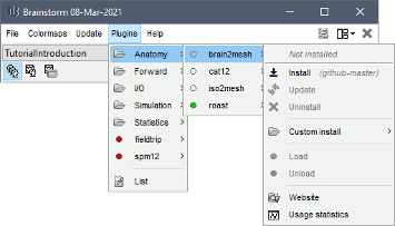
Using the Brainstorm plug-in system, download the following plugins :
NIRS > NIRSTORM : the core of NIRSTORM package
NIRS > MCXLAB-cl : a plugin for the estimation of the fNIRS forward model using Monte Carlo simulations of infrared light photons in the anatomical head model
Inverse > Brainentropy: our package dedicated to solving the fNIRS reconstruction inverse problem using the Maximum Entropy on the Mean framework
Downloading the dataset.
The total disk space required after data download and installation is ~1.3Go. The size is quite large because of the optical data that are required for the computation of the forward model. The dataset can be downloaded from: https://osf.io/md54y/?view_only=0d8ad17d1e1449b5ad36864eeb3424ed .
License: This tutorial dataset (fNIRS and MRI data) remains proprietary of the MultiFunkIm Laboratory of Dr Grova, at Concordia School of Health, Concordia University, Montreal. Its use and transfer outside the Brainstorm tutorial, e.g. for research purposes, is prohibited without written consent from our group. For questions please contact Dr. Christophe Grova: christophe.grova@concordia.ca
Data importation and preprocessing
Description of the data organization The data are organized using the following scheme according to BIDS standards:
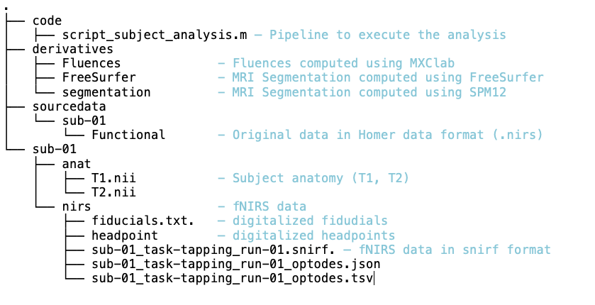
Data Importation
- Start Brainstorm (Matlab scripts or stand-alone version)
Select the menu File > Create new protocol. Name it "TutorialNIRS" and select the options: "No, use individual anatomy", "No, use one channel file per acquisition run (MEG/EEG)".
In terms of sensor configuration, fNIRS is similar to EEG and the placement of optodes may be subject-specific. Also, the channel definition will change during data processing, this is the reason why you should always use one channel file per acquisition run, even if the optode placement remains the same.
Importing anatomical data
Import anatomical data Following tutorials 1-2, import the subject anatomy segmented using freesurfer using the following fiducials coordinate in MRI coordinate:
Switch to the "anatomy" view of the protocol.
Right-click on the TutorialNIRS folder > New subject > sub-01
- Leave the default options you set for the protocol
Right-click on the subject node > Import anatomy folder:
- Set the file format: "Freesurfer + volumes atlases"
- Select the folder: nirstorm_tutorial_2024/derivatives/FreeSurfer/sub-01
- Number of vertices of the cortex surface: 15000 (default value)
- Answer "yes" when asked to apply the transformation.
- Set the 3 required fiducial points, indicated below in (x,y,z) MRI coordinates.
You can right-click on the MRI viewer > Edit fiducial positions > MRI coordinates, and copy-paste the following coordinates in the corresponding fields. Click [Save] when done.
- Nas : [ 131, 213, 117 ]
- Lpa : [ 51, 116, 80 ]
- Rpa : [ 208, 117, 86 ]
- Ac : [ 131, 128, 130 ]
- Pc : [ 129, 103, 124 ]
- Ih : [ 133, 135, 176 ]
- Once the anatomy is imported, make sure that the surface "mid_15002V" is selected (green). If it is not, right-click on it and select "set as default cortex". This will define the cortical surface on which fNIRS 3D reconstructions will be estimated.
- Resample the head mask to get a uniform mesh on the head. For that, right-click on the head mask and select remesh, then 10242 vertices. This allows us to get a uniform mesh on the head.
Your database should look like this:

Note that the elements that appear in green correspond to those used for later computations. It is important that the new head mask (remeshed) and the mid-surface (mid_15002V) are selected and appear green in your database.
Additionally, we defined the hand knob on the mid-surface. Open the mid surface, and use Atlas > Add scouts to Atlas and select the FreeSurfer annotation: NIRSTORM-data/derivatives/segmentation/sub-01/scout_hand.annot
Import fNIRS functional data
The Brainsight acquisition software produced the functional fNIRS data used in this tutorial and is available in the data subfolder of the fNIRS sample folder(nirstorm_tutorial_2024/sub-01/nirs). The data were exported according to the BIDS format: See https://bids-specification.readthedocs.io/en/stable/modality-specific-files/near-infrared-spectroscopy.html for a description of each file.
To import this dataset in Brainstorm:
- Go to the "functional data" view of the protocol.
Right-click on sub-01 > Review raw file Select file type NIRS: SNIRF (.snirf)
- Select file nirstorm_tutorial_2024/sub-01/nirs/sub-01_task-tapping_run-01.snirf
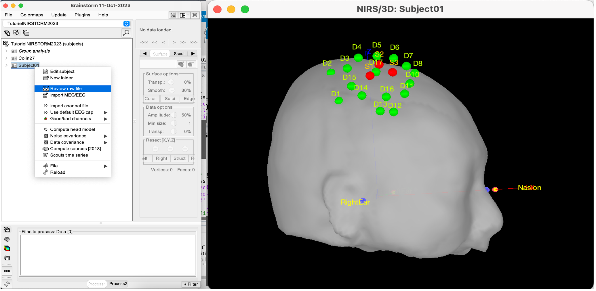
Co-registration of the fNIRS sensors with the anatomical MRI
In the same way as in the tutorial "Channel file / MEG-MRI coregistration", the registration between the MRI and the fNIRS is first based on the identification of three anatomical reference points identified in the MRI data and digitized together with the location of all sensors: the Nasion, Left and Right ears.
First, a rigid registration matrix (3 rotations, 3 translations) is estimated by aligning these three fiducials. Registration should then be refined either using additional head points (e.g. sensor locations or full digitalization of the head shape of the participant) or eventually using manual adjustment. We recommend using additional headpoints to refine the spatial registration.
The initial registration is based on the three fiducial points that define the Subject Coordinate System (SCS): nasion (NAS), left ear (LPA), right ear (RPA). The visual identification of these three anatomical landmarks on the anatomical MRI has been completed using the MRI viewer in the previous section.
Once sensors or the cap have been installed on the head of the participant, these same three fiducial points have also been digitized on the head of the participant before fNIRS acquisition, together with the location of all other sensors (fNIRS sources, detectors, and eventually EEG electrodes), once sensors have been installed.
We recommend using a tracking system to digitize the position of the 3 anatomical landmarks and sensor locations using a 3D tracking device (e.g. Polhemus or Brainsight neuronavigation system considered here). The positions of these points are saved in the fNIRS datasets (see fiducials.txt).
When the fNIRS recordings are loaded into the Brainstorm database, they are aligned on the anatomical MRI data using these anatomical landmark points: the NAS/LPA/RPA points digitized with Brainsight are matched with the ones we placed in the MRI Viewer.
To review the accuracy of fNIRS/MRI coregistration:
Right-click on NIRS-BRS sensors (97) > Display sensors > NIRS (pairs). This will display sources as red spheres and detectors as green spheres. Source/detector pairings are displayed as blue cylindrical lines.
Right-click on NIRS-BRS sensors (97) > Display sensors > NIRS (scalp). This will display sources as red spheres and detectors as green spheres
* To check the coregistration, Right-click on NIRS-BRS sensors (97) > MRI registration > check.
For more information about the coregistration accuracy and how to refine the coregistration, please consult "Channel file / MEG-MRI coregistration"
Review of recording
Select "sub-01 |- sub-01_task-tapping_run-01 |- Link to raw file -> NIRS -> Display time series". It will open a new figure with superimposed time courses of all fNIRS channels.

If coloring is not visible, then right-click on the figure and select "Montage > NIRS Overlay".
Indeed, brainstorm uses a dynamical montage, called NIRS Overlay, to regroup and color-code fNIRS time series depending on their wavelength (red: 830nm, green:686nm). Therefore, when clicking to select one curve for one wavelength, NIRSTORM will also select the other wavelength for the same pair.
Importing events
In this dataset, the events are directly encoded in the .snirf file and automatically imported by Brainstorm. In case your events are not encoded in your nirs file, you can import them manually (either from a specific channel, or external file). For more information, please consult https://neuroimage.usc.edu/brainstorm/Tutorials/EventMarkers
The events describing the task are currently extended events (having onset + duration). To facilitate trial averaging latter, it is recommended that you duplicate the events linked to your task and convert them to simple events using the start of each trial. Therefore, for this tutorial, duplicate the event 'tapping', convert it to simple, and rename it tapping/start.
Data analysis at the channel level
This section introduces the process of estimating the hemodynamic response to a finger-tapping task at the channel level.
This figure illustrates the full pipeline proposed in this tutorial, which will be described in further detail next.
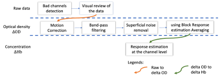
Pre-processing Pre-processing functions can be applied to fNIRS data files by adding the "Link to raw" file to the processing box or dragging and dropping it onto the box. Once it is in place, click on the "Run" button to execute the process. At this stage, both Brainstorm and NIRSTORM-specific processes (present under the nirs submenu), can be applied without any distinction to the nirs files.
Bad channel detection
Process: NIRS > Pre-process > Detect Bad channels
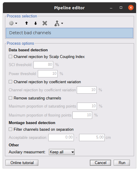
The Detect Bad Channels process aims at labeling each channel as good or bad based on a set of criteria:
- Negative value: Channel with negative values
- Scalp coupling index (SCI): SCI reflects the signal's correlation for each wavelength within the cardiac band.
- Power reflects the % of the power of the signal within the cardiac band. This process removes channels featuring Low SCI or low power within the cardiac band.
- Coefficient of variation (CV): reflects the dispersion of data points around the mean. This process removes channels featuring high CV.
- Saturating channels: Detect and remove channels showing saturation (how is this done) Source-Detector separation: This process removes the channels outside the acceptable source-detector distance range.
By default, if a wavelength of a channel is considered as bad, then the entire channel, i.e. signals from both wavelengths, is discarded.
Additionally, the process proposes to either keep or remove auxiliary channels (non-Nirs channels). Keep the auxiliary channels if your nirs system also recorded some peripherical measurements (heart rate, respiration …). In our case, there is no information in the auxiliary channel so we can discard them.
Raw to delta OD
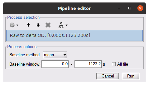
This function converts the light intensity to variations of optical density.
Process: nirs > dOD and MBLL > Raw to delta OD
Description:
Convert the fNIRS data from raw to delta OD delta OD=-10 log_10(I/I_0 ) Channels with negative values must have been removed (see bad channel detection section), before applying this log transformation.
Parameter: * Baseline window: Period of time used to estimate the baseline intensity I_0
Motion correction
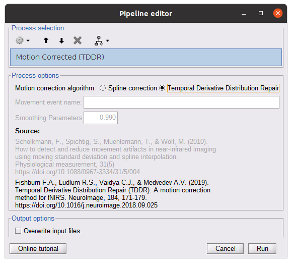
Process: nirs > pre-process > motion correction
Input: Raw data, delta OD, or delta Hb Description:
Description:
Apply a motion correction algorithm to the data. Two algorithms are implemented: (1) Spline correction (2) Temporal derivative distribution repair (TDDR)
Parameter:
Spline correction: After selecting motion visually on the fNIRS signal viewer, spline interpolation is used to smooth the signal during motion.[2]
- Movement event name: Name used to visually identify the motion Smoothing parameter: Value between 0 and 1 controlling the level of smoothness desired during the motion
Temporal derivative distribution repair: automatic motion correction algorithm that relies on the assumption that motion will introduce outliers in the temporal derivative of the optical density.[3]
There is no additional parameter
In this tutorial, we will be using Temporal derivative distribution repair.
Band-pass filter
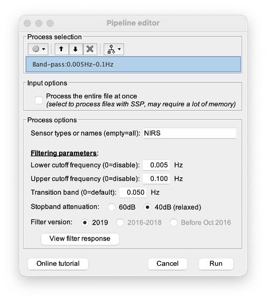
Process: pre-process > band-pass filter
Input: delta OD, or delta Hb Description:
Apply a finite impulse response (FIR) filter to the data. If you want to use an infinite impulse response filter (IIR), use the process from NIRS > pre-process > band-pass filter
Parameters:
- Sensor type: apply the FIR only to selected channels (useful if storing additional data in the auxiliary channels such as accelerometer, blood pressure …)
- Lower-cutoff / Upper-Cutoff: Cuttoff frequencies for the filter
- Transition band: Error margin for the filter before/after the cutoff.
Warning: it is important to specify this parameter for fNIRS data. Use the View filter response button to ensure that the design filter corresponds to what you desire.
- Stopband attenuation: Gain of the filter outside of the transition band. We recommend using 40 dB.
- Filter version: Version of the brainstorm implementation of the filter (We recommend using the 2019 version)
For more information about the filtering, see tutorial 3.
Note: we recommend always checking that the filter used corresponds to your expectation using the ‘View filter response button”
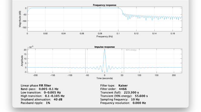
Regressing out superficial noise
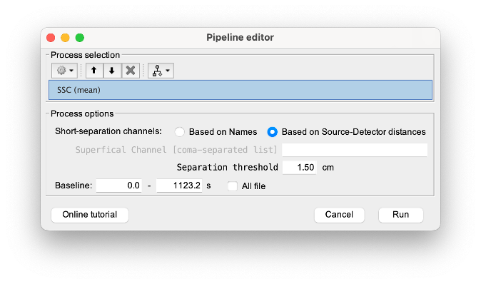
NIRS > Pre-process > Remove superficial noise
This process consists of regressing out superficial noise using the mean of all the channel identified as short-separation channels, following the methodology proposed in Delaire et al, 20244
Parameters:
- Method to select short-channel:
(1) based on Name: manually specify the name of the short-channels (eg. S1D17, S2D17…)
- (2) based on Source-Detector distance: use the Source-Detector distance to detect short-separation channels.
- (if 1) Superficial channels: list of short separation channels
- (if 2) Separation threshold: maximum Source-Detector distance to be considered as short-channel
- Baseline: Segment of the baseline signal that is considered to calibrate the superficial noise removal procedure. Select a window relatively free of motion. This is mainly useful for long-duration recordings, or when a part of your signal is heavily corrupted with motion.
Window averaging
The objective is to analyze the response produced by the motor paradigm. The following section presents how to analyze an fNIRS-elicited hemodynamic response by averaging single trials, therefore it corresponds to tutorials 15 and 16, presenting how to analyze a bioelectrical evoked response using EEG/MEG. We recommend the reader to consult those two tutorials for further details.
To estimate the hemodynamic response produced by the motor paradigm, we will extract epoch data locked on the motor paradigm starting 10s before the task and ending 30s after the beginning of the paradigm.
Use the import in database tool with the following parameters.
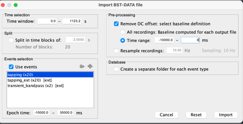
The Epoch time should range from -10s to 30s (i.e. -10,000 ms to 30,000 ms). This means that we will extract data segments 10 seconds before the stimulation event to check for signal stability, and 30 seconds after stimulation to observe the return to baseline of the hemodynamic response. Remove DC offset will:
* Compute the average of each channel over the baseline (pre-stimulus interval: [-10 000, 0]ms) Subtract it from the channel at every time instant (full epoch interval: [-10 000,+ 30 000]ms). This option removes the baseline value of each sensor.
If you are expecting a response to start before the time 0; make sure to set the pre-stimulus interval accordingly to not contain the start of the response.
⚠️ Please note that in Brainstorm the time is specified in milliseconds and not in seconds. To indicate a time of 10 seconds, the user should then write 10,000ms. This comes from the fact that the software is mainly developed for EEG/MEG where the response is occurring at the millisecond scale.
This import will create 20 files, each corresponding to an individual trial, which you can examine separately. Any trial with excessive movement can be rejected by right-clicking on it and selecting the "Reject trial" option. In our example, we want to reject the first trial as it is contaminated by the transient bandpass filter effect.
To calculate the average response, drag and drop the 20 files into the processing box, which will display "tapping (20 files) [19]". The number 19 indicates that only 19 out of the 20 files will be used (since we rejected trial #1).
You can then visualize the resulting average fNIRS response by inspecting the AvgStderr file: "tapping (19)".
Delta OD to delta [HbO], [HbR] & [HbT]
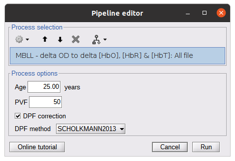
This process converts the optical density changes to changes in concentration of oxy-, deoxy-, and total hemoglobin. To perform this conversion, we apply the modified Beer-Lambert law using the method described in Scholkmann et al, 20135 to estimate the differential path length factor (DPF). Tuning the differential path length factor depends on the age of the participant and the wavelength. The partial volume factor (PVF) is also corrected. Most of the software recommends using 50 as a factor for the PVF.
Uncorrected data can also be calculated by unchecking the DPF correction.
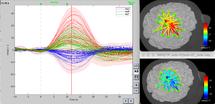
Data analysis on the cortical surface
In the previous section, we were able to estimate and analyze the hemodynamic response elicited by a finger tapping task at the sensor level. The objective of this section is to reconstruct the response, i.e. HbO, HbR, HbT fluctuations, along the cortical surface beneath our fNIRS montage. Two diffuse optical tomography (DOT) methods have been implemented and validate in NIRSTORM: (i) the Minimum Norm Estimate (MNE) or the Maximum Entropy on the Mean. (add the refs to both methods) For more information on the use of these inverse problem solvers on EEG/MEG data please consult Tutorial 22: Source Estimation and Best: Brain Entropy in space and time.
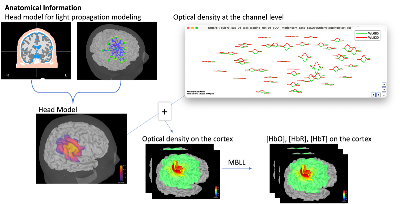
Illustration of the pipeline for fNIRS 3D reconstruction and analysis on the cortical surface.
Computation of the fNIRS forward model
The process of reconstructing fNIRS responses along the cortical surface relies on solving what is known as an ill-posed inverse problem. However, before proposing methods to solve this inverse problem, it is mandatory to solve the well-posed forward problem, which consists in modelling in a realistic manner the propagation of infrared light inside the head. Solving the fNIRS forward model will consist in generating a sensitivity matrix that maps how a local change in light absorption along the cortical region will impact the measured changes in optical density on every scalp fNIRS channels.
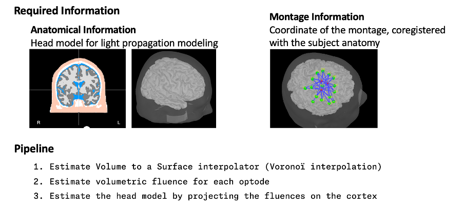
Segmentation of the MRI
To estimate the propagation of infrared light inside the head, we need to compute two preliminary maps: (i) a volumic segmentation of the head into 5 tissues segmentation (skin, CSF, grey matter, white matter). This can be done using SPM. Right-click on the T1 MRI and use MRI segmentation > SPM12. Answer ‘yes’, to use the T2 image to refine the MRI segmentation (mention that they should do this if they have both T1 and T2 available, … what happens if we have only T1, also if we have both I guess we should first co-register them or is it done in SPM12 pipeline). Rename the segmentation (what is the name of SPM12 output) to ‘segmentation_5tissues’. The name is important for further process.
For the tutorial, we are going to import a pre-computed segmentation of the MRI using a combination of SPM12 and Freesurfer. To learn more about the segmentation, consult the advanced tutorial on segmentation: https://neuroimage.usc.edu/brainstorm/Tutorials#Advanced_tutorials
For this tutorial, we are providing a pre-computed 5-tissue segmentation. To import this pre-computed segmentation,
Right-click on the subject node > Import MRI Set the file format: Volume atlas (subject space)
- Select the file nirstorm_tutorial_2024/derivatives/segmentation/sub-01/segmentation_5tissues.nii using Volume atlas (subject space) for the file format
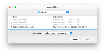
Estimate Volume to a Surface interpolator (Voronoï interpolation)
In this step, your anatomical tab within Brainstorm database should be similar to the following one :
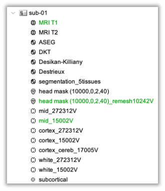
It is important that the correct T1 MRI and surfaces are selected as default. Also, a segmentation named ‘segmentation_5tissues’ should be present in the database (the exact syntax of the name of the segmentation is important).
The Voronoi interpolator allows to project volumetric data on the cortical surface. This will be used to project the volumetric fluence data calculated in the MRI volume space along the cortical surface.
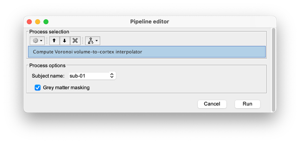
To compute the Voronoi interpolator:
- Click on run, without any file in the process box
Under NIRS > Sources, select Compute Voronoi volume-to-cortex interpolator.
- Then select the subject, and use the Grey matter masking option.
Computation of the fluences
The estimation of the fNIRS forward model is done in two steps:
- The estimation of the fluences for each optode (source or detector) The estimation of the forward model from the fluences.
Fluence data reflecting light propagation from any surface head vertex can be estimated by Monte Carlo simulations of photon transport within a realistic head model, using MCXlab software developed by (Fang and Boas, 20096). To compute the fNIRS forward model, sensitivity values in each voxel for each channel (i.e. a source-detector pair) are then computed by multiplication of fluence rate distributions using the adjoint method according to the Rytov approximation as described in (Boas et al., 20027). Within NIRSTORM, we prepared an interface that can call MCXlab and compute fluences corresponding to a set of vertices along the head surface. See the MCXlab documentation for further details. To allow faster fluence computations, we recommend you to use the GPU implementation of MCXlab. Before launching fluence computations, you need to load the plugin called MCXlab-cl (or MCXlab-cuda if your GPU supports CUDA).
To estimate the fluence, drag and drop the average estimated hemodynamic response to the tapping to the process box and call NIRS > Source > Compute fluences.
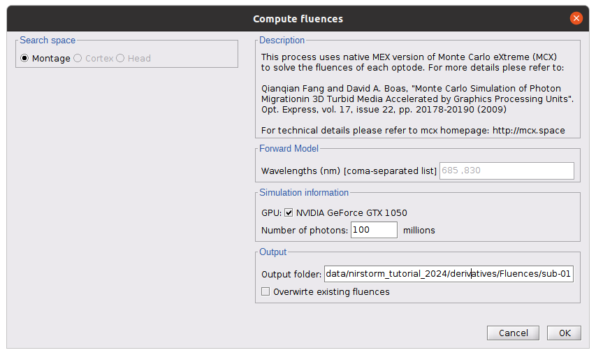
The key parameters to consider are as follows:
- Number of photons: Number of photons used for Monte Carlo simulations. A higher number of photons will improve the quality of the estimation but will require more time. We recommend using at least 10 million photons.
- GPU/CPU: Select the CPU/GPU used for the simulation. You can select multiple.
- Output directory: where the fluence data will be stored.
In our case, select the folder: NIRSTORM-data/derivatives/Fluences/sub-01 …
Computing head model from fluences
Once the fluences are estimated for every fNIRS source or detector in your fNIRS montage, the fNIRS forward model can be computed using NIRS > Source > Compute head model from fluences.
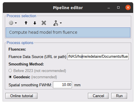
The parameters are:
- Fluence Data source: Path where the fluences are stored (same directory as the previous process). In this tutorial, fluences were pre-computed under NIRSTORM-data/derivatives/Fluences/sub-01
Smoothing method: After the projection of the fluence on the cortex, spatial smoothing is applied. The filter was changed in 2023 (see https://github.com/brainstorm-tools/brainstorm3/pull/645 for more information). We recommend using the new filter: Geodesic.
- Spatial smoothing FWHM: Amount of spatial smoothing to apply. If using geodesic, we recommend using 10 mm. If you are using the filter ‘Before 2023’, use 5 mm.
Investigating the light sensitivity of the montage
To visualize the sensitivity of the selected montage along the cortical surface, use the process NIRS > Source > Extract sensitivity surfaces from the head model:
Drag and drop any file that is present in the same folder as the forward model and use the process NIRS > sources > Extract sensitivity maps from the head model
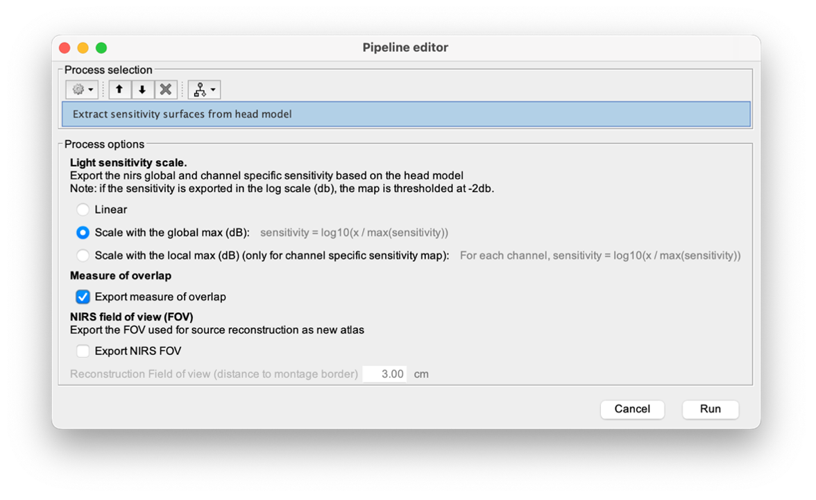
The process will generate the following maps for each wavelength:
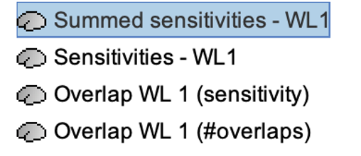
Montage Sensitivity: Sensitivities and Summed sensitivities report the measure of light sensitivity of the montage
Sensitivities: Sensitivity map for each channel, this is a spatiotemporal matrix, to move from one channel to the other one needs to … (to explain) Summed sensitivities: Overall sensitivity map of the whole montage (sum of the sensitivity maps of all the channels)

Measure of spatial overlap between fNIRS channels: Overlap (#overlap and sensitivity) reports two measures quantifying the amount of overlapping channels in the montage. To do so, a threshold must first be set, considering either the minimum number of channels sensitive to a specific cortical region or the minimum sensitivity required to receive signals from that region.
Overlap (sensitivity): When setting the threshold to the expected minimum number Nc of channels sensitive to a region, NIRSTORM reports, for each vertex, the minimum light sensitivity (in dB) achieved by the Nc most sensitive channels
Overlap (#overlap): when specifying a threshold on the expected minimum light sensitivity to reach a specific region, the algorithm reports for each vertex how many channels are sensitive to light absorption changes occurring within that specific vertex (above the specified threshold)
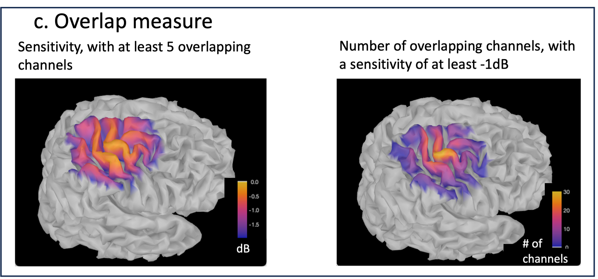
fNIRS 3D reconstruction: solving the fNIRS inverse problem
fNIRS 3D Reconstruction consists of solving an anil-posed inverse problem, which involves inverting an advanced model to reconstruct local cortical changes in hemodynamic activity within the brain, from scalp measurements (Arridge, 2011)8. The inverse problem is ill-posed and has an infinite number of solutions. To obtain a unique solution, adding regularization is required. We implemented two algorithms to reconstruct fNIRS data in NIRSTORM:
- the minimum norm estimate (MNE) [see ref 9]
- the maximum entropy over the mean (MEM) [ see ref 1,10].
Inverse problem using MNE
The Minimum Norm Estimate (MNE) is one of the most used reconstruction methods in fNIRS tomography. It consists of minimizing the L2 norm of the reconstruction error with Tikhonov regularization (Boas et al., 2004).
Note that in our MNE implementation, we considered the L-curve method (Hansen, 2000) to tune the regularization hyperparameters in the MNE model.
To apply MNE fNIRS reconstruction, use source > Source reconstruction – wMNE on the file AvgStderr: tapping_02 (19).
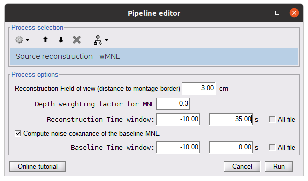
The parameters for this process are as follows:
- Reconstruction field of view: 5 cm. We only reconstruct the activity on the vertex near the montage.
- Depth weighting factor for MNE: 0.3. This takes into account that fNIRS measurements have greater sensitivity in the superficial layer and are used to correct for signal sources that may be deeper.
- Compute noise covariance: If this option is selected, the noise covariance matrix is calculated based on the defined reference window below. The covariance matrix is defined using a diagonal matrix with a specific value per channel. If not specified, the identity matrix will be used to model the noise covariance.
Further details on our implementation of depth-weighted MNE are available in Cai et al Sci. Rep 2022 [10]
The results of the reconstruction will be listed under "AvgStd FingerTapping (19)".
Expand "AvgStd FingerTapping (19)" to view the MNE reconstruction results.
Double-click on the files "MNE sources - HbO" and "MNE sources - HbR" to review the reconstructed maps. To display the reconstructed time courses of HbO/HbR along the cortical surface, define a region for extracting these time courses.
To do so, switch to the "scout" tab in the view control panel. Click on the scout named "Hand". (explain how this one was defined and mention that one can define their own scout as well) In the "time-series options" section at the bottom, select "Values: Relative".
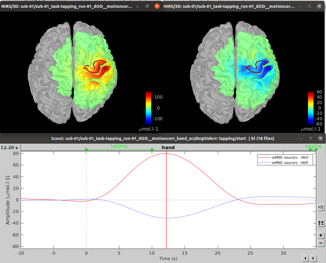
Inverse problem using cMEM
The MEM framework was first proposed by (Amblard et al., 2004)13, then applied and evaluated in the context of electroencephalography (EEG) and magnetoencephalography (MEG) source imaging (Grova et al., 200614; 15 et al., 2013). To see how it was adapted for fNIRS, consult [1,10].
Please refer to the tutorial Maximum Entropy on the Mean (MEM): https://neuroimage.usc.edu/brainstorm/Tutorials/TutBEst for more details on MEM.
MEM framework was specifically designed and evaluated for its ability to localize the underlying generators of EEG/MEG data along the cortical surface while featuring the unique property of recovering accurately the spatial extent of the underlying generators [16–21]
To use MEM, use NIRS > Source > Compute sources: Best. on the file AvgStderr: tapping_02 (19).
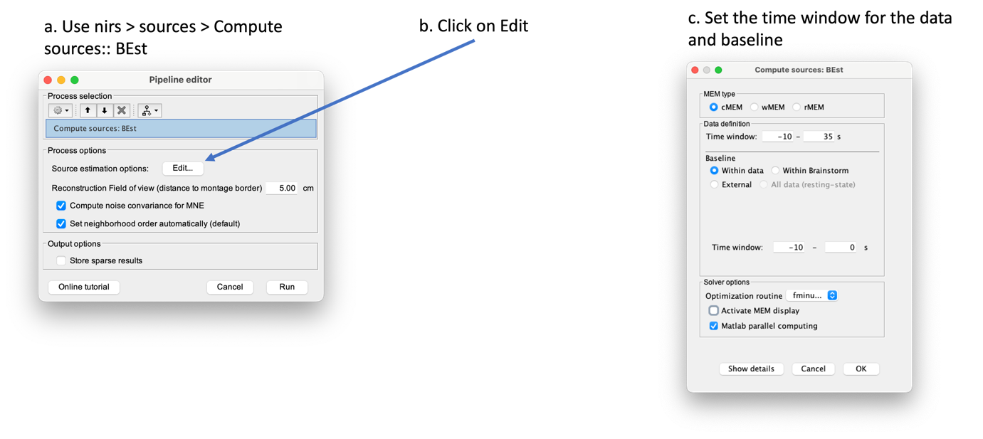
Here you should use the following options:
- MEM type: cMEM
- Data definition:
- Time windows: -10 – 35 s
- Baseline:
- Within data: we will be extracting the baseline from the data
- Time window: -10 - 0 s
Similarly, to MNE, you can After applying MEM 3D reconstruction, we obtain the following result:
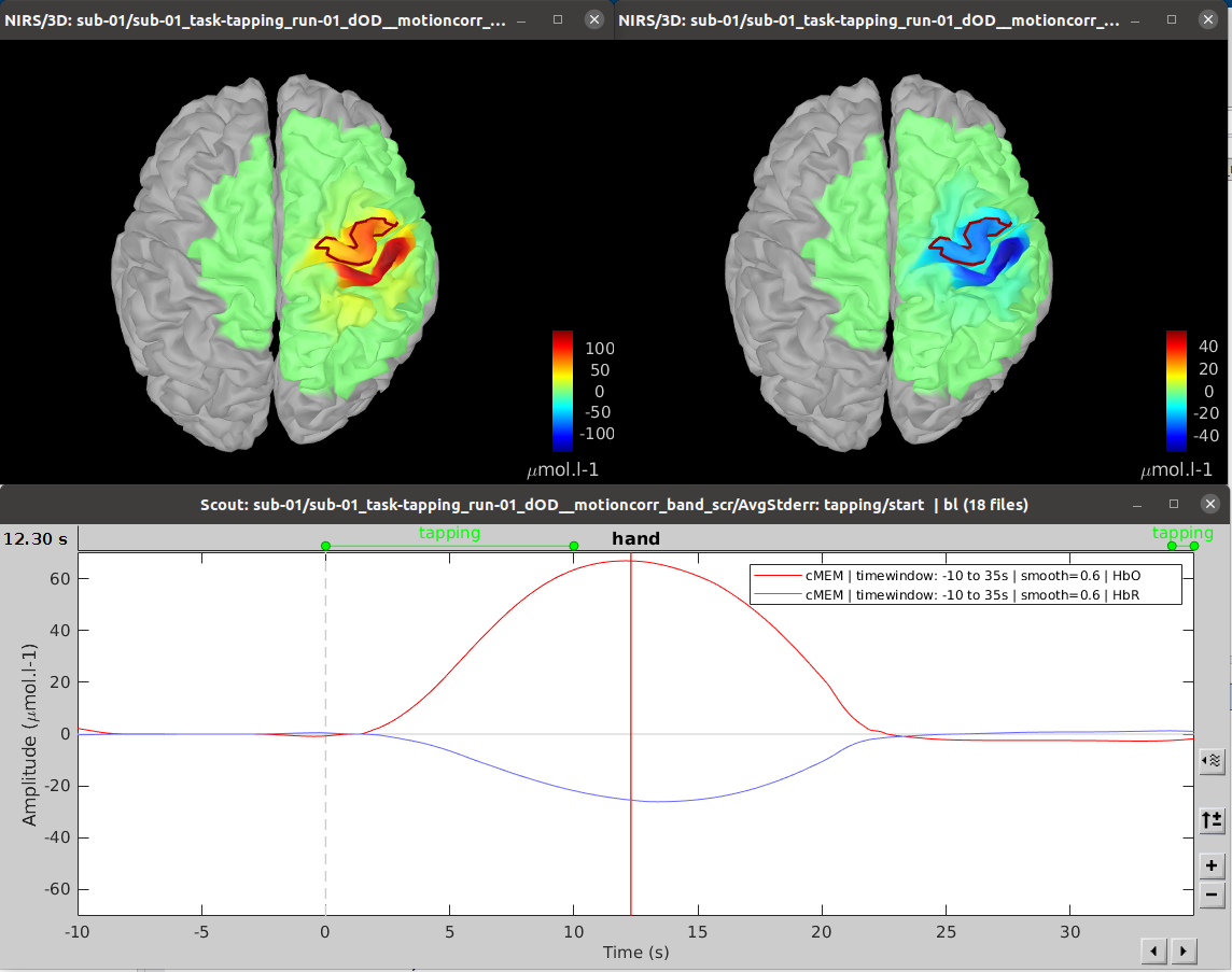
References
1. Cai Z, Uji M, Aydin Ü, et al. Evaluation of a personalized functional near infra-red optical tomography workflow using maximum entropy on the mean. Hum Brain Mapp. 2021;42(15):4823-4843. doi:10.1002/hbm.25566
2. Scholkmann F, Spichtig S, Muehlemann T, Wolf M. How to detect and reduce movement artifacts in near-infrared imaging using moving standard deviation and spline interpolation. Physiol Meas. 2010;31(5):649-662. doi:10.1088/0967-3334/31/5/004
3. Fishburn FA, Ludlum RS, Vaidya CJ, Medvedev A V. Temporal Derivative Distribution Repair (TDDR): A motion correction method for fNIRS. Neuroimage. 2019;184(September 2018):171-179. doi:10.1016/j.neuroimage.2018.09.025
4. Delaire É, Vincent T, Cai Z, et al. NIRSTORM: a Brainstorm extension dedicated to functional Near Infrared Spectroscopy (fNIRS) data analysis, advanced 3D reconstructions, and optimal probe design. bioRxiv. Published online 2024. doi:10.1101/2024.09.05.611463
5. Scholkmann F, Wolf M. General equation for the differential pathlength factor of the frontal human head depending on wavelength and age. J Biomed Opt. 2013;18(10):105004. doi:10.1117/1.jbo.18.10.105004
6. Fang Q, Boas DA. Monte Carlo Simulation of Photon Migration in 3D Turbid Media Accelerated by Graphics Processing Units. Opt Express. 2009;17(22):20178. doi:10.1364/oe.17.020178
7. Boas DA, Culver JP, Stott JJ, Dunn AK. Three dimensional Monte Carlo code for photon migration through complex heterogeneous media including the adult human head. Opt Express. 2002;10(3). doi:10.1364/oe.10.000159
8. Arridge SR. Optical tomography in medical imaging. Inverse Probl. 1999;15(2). doi:10.1088/0266-5611/15/2/02 9. Lin FH, Witzel T, Ahlfors SP, Stufflebeam SM, Belliveau JW, Hämäläinen MS. Assessing and improving the spatial accuracy in MEG source localization by depth-weighted minimum-norm estimates. Neuroimage. 2006;31(1):160-171. doi:10.1016/j.neuroimage.2005.11.054 10. Cai Z, Machado A, Chowdhury RA, et al. Diffuse optical reconstructions of functional near infrared spectroscopy data using maximum entropy on the mean. Sci Rep. 2022;12(1):1-18. doi:10.1038/s41598-022-06082-1
11. Boas DA, Dale AM, Franceschini MA. Diffuse optical imaging of brain activation: Approaches to optimizing image sensitivity, resolution, and accuracy. Neuroimage. 2004;23(SUPPL. 1). doi:10.1016/j.neuroimage.2004.07.011
12. Hansen PC. The L-Curve and its Use in the Numerical Treatment of Inverse Problems. In: In Computational Inverse Problems in Electrocardiology, Ed. P. Johnston, Advances in Computational Bioengineering. WIT Press; 2000:119-142.
13. Amblard C, Lapalme E, Lina JM. Biomagnetic Source Detection by Maximum Entropy and Graphical Models. IEEE Trans Biomed Eng. 2004;51(3):427-442. doi:10.1109/TBME.2003.820999
14. Grova C, Daunizeau J, Lina JM, Bénar CG, Benali H, Gotman J. Evaluation of EEG localization methods using realistic simulations of interictal spikes. Neuroimage. 2006;29(3).doi:10.1016/j.neuroimage.2005.08.053
15. Chowdhury RA, Lina JM, Kobayashi E, Grova C. MEG Source Localization of Spatially Extended Generators of Epileptic Activity: Comparing Entropic and Hierarchical Bayesian Approaches. PLoS One. 2013;8(2). doi:10.1371/journal.pone.0055969
16. Chowdhury RA, Merlet I, Birot G, et al. Complex patterns of spatially extended generators of epileptic activity: Comparison of source localization methods cMEM and 4-ExSo-MUSIC on high resolution EEG and MEG data. Neuroimage. 2016;143:175-195. doi:10.1016/j.neuroimage.2016.08.044
17. Heers M, Hedrich T, An D, et al. Spatial correlation of hemodynamic changes related to interictal epileptic discharges with electric and magnetic source imaging. Hum Brain Mapp. 2014;35(9):4396-4414. doi:10.1002/hbm.22482
18. Grova C, Aiguabella M, Zelmann R, Lina JM, Hall JA, Kobayashi E. Intracranial EEG potentials estimated from MEG sources: A new approach to correlate MEG and iEEG data in epilepsy. Hum Brain Mapp. 2016;37(5). doi:10.1002/hbm.23127
19. Abdallah C, Hedrich T, Koupparis A, et al. Clinical Yield of Electromagnetic Source Imaging and Hemodynamic Responses in Epilepsy: Validation With Intracerebral Data. Neurology. Published online 2022.
20. Pellegrino G, Hedrich T, Chowdhury RA, et al. Clinical yield of magnetoencephalography distributed source imaging in epilepsy: A comparison with equivalent current dipole method. Hum Brain Mapp. 2018;39(1). doi:10.1002/hbm.23837
21. Pellegrino G, Hedrich T, Porras-Bettancourt M, et al. Accuracy and spatial properties of distributed magnetic source imaging techniques in the investigation of focal epilepsy patients. Hum Brain Mapp. 2020;41(11):3019-3033. doi:10.1002/hbm.24994
