|
Size: 1487
Comment:
|
Size: 15073
Comment:
|
| Deletions are marked like this. | Additions are marked like this. |
| Line 1: | Line 1: |
| = Tutorial 14: Noise covariance = ''Authors: Francois Tadel, Elizabeth Bock, John C Mosher, Sylvain Baillet'' |
= Tutorial 21: Noise and data covariance matrices = ''Authors: Francois Tadel, Elizabeth Bock, John C Mosher, Richard Leahy, Sylvain Baillet'' Modeling and measuring certain charateristics of the noise contaminating the data is beneficial to source estimation. For instance, minimum norm estimators can integrate second-order sample statistics of sensor noise (summarized into a '''noise covariance matrix''', see below). Beamformers further require similar sample statistics for the data portion of interest (summarized into a '''data covariance matrix'''). This first section of this tutorial explains how to obtain a noise covariance estimate from MEG empty room recordings. |
| Line 6: | Line 8: |
| From continuous tutorials: | == Noise covariance == Instrumental noise ("sensor noise") can be readily captured in MEG using two or more minutes of empty room measurements. We encourage the use of noise recordings collected the same day as the subject's recordings (if possible just before the session) and pre-processed in the same manner (with same sampling rate and same frequency filters applied) as the participant data. In this study we have already prepared a 2-min segment of noise recordings that we will use to estimate noise covariance sample statistics. |
| Line 8: | Line 11: |
| === Noise covariance matrix === To estimate the sources properly, we need an estimation of the noise level for each sensor. A good way to do this is to compute the covariance matrix of the concatenation of the baselines from all the trials in both conditions. |
Right-click on the entry for '''noise recordings''' '''> Noise covariance'''. Available menus: |
| Line 11: | Line 13: |
| * Select at the same time the two groups of trials (right and left). To do this: hold the Control (or Cmd on Macs) key and click successively on the Right and the Left trial lists. * Right-click on one of them and select: Noise covariance > Compute from recordings. Set the baseline to '''[-104,-5] ms''', to consider as noise everything that happens before the beginning of the stimulation artifact. Leave the other options to the default values. Click on Ok. * This operation computes the noise covariance matrix based on the baseline of all the good trials (199 files). The result is stored in a new file "Noise covariance" in the ''(Common files)'' folder. |
* '''Compute from recordings''': Use the selected recordings to estimate noise covariance statistics. * '''No noise modeling''': Use an identity matrix as noise covariance. This option is useful when no noise recording is available (e.g. ongoing EEG without any baseline of no interest). * '''Import from file''': Use noise covariance statistics available from another source (e.g., obtained using the MNE software.) * '''Import from Matlab''': Import any [Nchannels x Nchannels] matrix as noise covariance matrix from the Matlab workspace. <<BR>><<BR>> {{attachment:noisecov_popup.gif||height="231",width="408"}} |
| Line 15: | Line 18: |
| {{http://neuroimage.usc.edu/brainstorm/Tutorials/TutRawAvg?action=AttachFile&do=get&target=noisecov.gif|noisecov.gif|class="attachment"}} | Select the menu '''Noise covariance > Compute from recordings'''. Available options: * '''Files''': The top part of this window shows a summary of the files that have been selected to estimate the noise: 1 file of 120s at 600Hz. Total number of time samples in selected file: 72,000. We can also choose to use only a portion of this file, with the option "baseline". The large continuous files are split in blocks of a maximum of '''10,000 samples''' that are then processed as different files. * '''Remove DC offset''': All the selected blocks of data are baseline corrected and concatenated to form a large matrix "F". There are two options for baseline correction:<<BR>>'''Block by block''': The average value of each channel is subtracted from each block before concatenating files together. <<BR>>Let Fi contain data from block #i: F = Concatenate[Fi - mean(Fi)].<<BR>>'''Global''': The average value of each channel is removed after concatenation (same correction for all blocks). <<BR>>F = Concatenate[Fi] - mean(Concatenate[Fi]). * The sample noise covariance is computed from F: '''NoiseCov = F * F' / Nsamples''' <<BR>><<BR>> {{attachment:noisecov_options.gif||height="278",width="346"}} For this tutorial, keep the default options and click on ['''OK''']. * One new file is created and appears under the noise data folder, next to the channel file. The corresponding contextual menus are: * '''Display as image''': Opens a display of the noise covariance matrix as an indexed image (same as double-click on file). This can be useful to quickly control the quality of the recordings: for instance, noisier channels appear as rows/columns marked in red. * '''Copy to other conditions''': Copy the file obtained to all the other folders of the same subject, to avoid re-computing the noise covariance statistics again for each folder from the same session. * '''Copy to other subjects''': Copy this file to all the folders of all the subjects in the protocol. * You can also copy a noise covariance file to another folder just like any other file: <<BR>>Right-click > File > Copy/Paste, or keyboard shortcuts Ctrl+C/Ctrl+V. <<BR>><<BR>> {{attachment:noisecov_file.gif||height="141",width="315"}} {{attachment:noisecov_display.gif||height="170",width="148"}} Right-click on the the noise covariance file > '''Copy to other folders''': We need this file in the two folders where the epochs were imported before we compute the respective source models. . {{attachment:noisecov_copy.gif||height="225",width="212"}} <<TAG(Advanced)>> == Variations on how to estimate sample noise covariance == The sample noise covariance matrix is straightforward to otbain. Brainstorm's interface features a lot of flexibility to select the files and time windows used to calculate the sample statistics. You need to have a clear understanding of the concept of "noise" to pick the best possible option. We support the notion that noise covariance accounts for contaminants that remain present in the data after pre-processing is complete. Hence it is not meant to account for eye blinks, heartbeats, muscle artifacts, flat or bad channels and noisy segments: all these the above need to be taken care of during previous preprocessing steps, as show in previous tutorial sections. The noise covariance entry is to account for remaining and stationnary instrumental, sensor and environmental noise components. For this reason, the ideal scenario is to use segments of recordings that contain exclusively this type of contaminant, or segments of recordings deemed not to contain any of brain signals of interest. This section is advanced reading material that can be used as a reference in a different experimental context. ==== The case of MEG ==== '''Empty room''': actual noise measurements (due to the instrument, environment) using empty-room conditions (no subject under the MEG helmet) are possible in MEG. We recommend you obtain 2 to more minutes of empty-room data right before bringing the subject in the MEG room, or right after the experiment is finished. .<<BR>>You can verify quatitatively how stable and reproducible is the noise covariance estimated (e.g., during the day/week). You may be in a "quiet environment" allowing that you re-use the same noise recordings and therfore, noise covariance matrix, for all runs and subjects acquired on the same day. '''Resting baseline''': Alternatively, when studying evoked responses (aka event-related responses), you can use a few minutes of recordings where the subject is resting, ie. not performing the task. Record those resting segments before or after the experiment, or before/after each run. This approach considers the resting brain activity as "noise", the sources estimated for the evoked response are going to be preferentially the ones that were not activated during the resting period. '''Pre-stimulation baseline''': It can also be a valid approach to use the pre-stimulation baseline of the individual trials to estimate the noise covariance. But keep in mind that in this case, everything in your pre-stimulation baseline is going to be attenuated in the source reconstruction, noise and brain activity. Therefore, your stimuli have to be distant enough in time so that the response to a stimulus is not recorded in the "baseline" of the following one. For repetitive stimuli, randomized delays between stimuli can help avoiding expectation effects in the baseline. ==== EEG ==== The EEG case is typically more complicated. It is not possible to estimate the noise of the sensors only. Only the two other approaches described for the MEG are still valid: <<BR>>'''resting baseline''' and '''pre-stimulation baseline'''. The noise level of the electrode recordings depends primarily on the quality of the connection with the skin, which varies a lot from a subject to another, or even during the acquisition of one single subject. The conductive gel or solution used on the electrodes tends to dry, and the electrode cap can move. Therefore, it is very important to use one channel file per subject, hence one noise covariance per subject. In some specific cases, if the quality of the recordings varies a lot over the time, it can be interesting to split long recordings in different runs, with different noise covariance matrices too. ==== EEG and resting state ==== When studying the resting brain, you cannot use resting recordings as a noise baseline. For MEG the best choice is to use empty room measurements. For '''EEG''', you can chose between two different approaches: using the sensors variance, or not using any noise information.<<BR>>'''Option #1''': Calculate the covariance over a long segment of the resting recordings, but save only the diagonal, ie. the variance of the sensors. This option is available in the advanced options of the source computation: select the option "Diagonal noise covariance".<<BR>>'''Option #2''': Select "No noise modeling" in the popup menu. This would use an identity matrix instead of a noise covariance matrix (equal, unit variance of noise on every sensor). In the inverse modeling, this is equivalent to the assumption that the noise in the recordings is homoskedastic, and equivalent for all the sensors. The problem with this approach is that an electrode with a higher level of noise is going to be interpreted as a lot of activity in its region of the brain. ==== Noise and epilepsy ==== Analyzing a single interictal spike, using either EEG and MEG data, we are faced with a similar problem in defining what is noise. Even the brain activity before and after the spike can be very informative about the spike's generation, particularly if it is part of a sequence of interictal activity that precedes ictal (seizure) onset. Defining a segment of time adjacent the spike as "background" may not be practical. In practice, however, we can often find a period of time of spontaneous brain activity in the recordings that appears adequate for declaring as background, even in the epileptic patient. As discussed above, MEG has the additional option of using empty room data as a baseline, an option not available in EEG. We thus have the same options as above:<<BR>>'''Option #1a''': Compute the noise covariance statistics from blocks of recordings away from the peak of any identified interictal spike, and keep only the diagonal (the variance of the sensors).<<BR>>'''Option #1b:''' If a large period of time is available, calculate the full noise covariance.<<BR>>'''Option #2(MEG): '''Use empty room data as the baseline.<<BR>>'''Option #3''': Select "No noise modeling" in the popup menu (identity matrix, unit variance of noise on every sensor). <<TAG(Advanced)>> == Recommendations == * '''Long noise recordings''': In order to get a good estimation of the noise covariance, we need a significant number of time samples, at least '''N*(N+1)/2''', where N is the number of sensors. This means about 40s for CTF275 recordings at 1000Hz, or 20s for 128-channel EEG at 500Hz. Always try to use as much data as possible for estimating this noise covariance. * '''Do not import averages''': For this reason, you should never compute the noise covariance matrix from averaged responses. If you want to import recordings that you have fully pre-processed with another program, we recommend you import the individual trials and use them to compute the noise covariance. If you can only import the averaged responses in the Brainstorm database, you have to be aware that you may get poor results in the source estimation. * '''Using one block''': If you want to use a segment of "quiet" recordings in a continuous file: right-click on the continuous file > Noise covariance > Compute from recordings, then copy the noise covariance to the other folders. This is the case described in this tutorial. * '''Use single trials''': If you want to use the pre-stimulation baseline of the single trials, first import the trials in the database, then select all the groups of imported trials at once, right-click on one of them > Noise covariance > Compute from recordings, and finally copy the file to the other folders. * '''Using multiple continuous blocks''': This is similar to the single trial case. Import in the database all the blocks you consider as quiet resting baselines, then select all the imported blocks in the database explorer > Noise covariance > Compute from recordings. <<TAG(Advanced)>> == Data covariance == The beamforming approach to source localization requires a data covariance in input. The computation of a data covariance matrix is very similar to a noise covariance matrix, except that you need to target the segments of recordings of interest instead of the noise. In the case of an event-related study, you can consider all the recordings in a range of latencies after the stimulation corresponding to the effect you want to localize in the brain. * For '''run#01''', select '''all the trials''', right-click > '''Data covariance > Compute from recordings'''. <<BR>><<BR>> {{attachment:datacov_popup.gif||height="180",width="407"}} * We need to specify two time windows from these recordings:<<BR>>'''Baseline''': Pre-stimulus time, used for DC offset correction (subtracts the baseline mean).<<BR>>'''Data''': Time segment of interest (let's use all the time available post-stimulus).<<BR>><<BR>> {{attachment:datacov_options.gif||height="329",width="365"}} * Repeat the operation for '''run#02'''. <<BR>><<BR>> {{attachment:datacov_files.gif||height="238",width="208"}} <<TAG(Advanced)>> == On the hard drive == Right-click on any noise covariance file > File > View file contents: . {{attachment:noisecov_contents.gif||height="175",width="487"}} ==== Structure of the noise/data covariance files: noisecov_*.mat / ndatacov_*.mat ==== * '''Comment''': String displayed in the database explorer to represent this file. * '''NoiseCov''': [nChannels x nChannels] noise covariance: '''F * F' ./ (nSamples-1)'''<<BR>>Unknown values are set to zero. * '''FourthMoment''': [nChannels x nChannels] fourth order moments: '''F.<<HTML(^)>>2 * F'.<<HTML(^)>>2 ./ (nSamples-1) ''' * '''nSamples''': [nChannels x nChannels] number of time samples that were used for each pair of sensors. This is not necessarily the same value everywhere, some channels can be bad only for a few trials. '''Related functions''' * '''process_noisecov'''.m: Function for process "Sources > Compute covariance (noise or data)" * '''bst_noisecov'''.m: Computes the data/noise covariance matrices. * '''panel_noisecov'''.m: Options panel. <<TAG(Advanced)>> == Additional documentation == * Forum: EEG reference: http://neuroimage.usc.edu/forums/showthread.php?1525#post6718 <<HTML(<!-- END-PAGE -->)>> |
Tutorial 21: Noise and data covariance matrices
Authors: Francois Tadel, Elizabeth Bock, John C Mosher, Richard Leahy, Sylvain Baillet
Modeling and measuring certain charateristics of the noise contaminating the data is beneficial to source estimation. For instance, minimum norm estimators can integrate second-order sample statistics of sensor noise (summarized into a noise covariance matrix, see below). Beamformers further require similar sample statistics for the data portion of interest (summarized into a data covariance matrix). This first section of this tutorial explains how to obtain a noise covariance estimate from MEG empty room recordings.
Contents
Noise covariance
Instrumental noise ("sensor noise") can be readily captured in MEG using two or more minutes of empty room measurements. We encourage the use of noise recordings collected the same day as the subject's recordings (if possible just before the session) and pre-processed in the same manner (with same sampling rate and same frequency filters applied) as the participant data. In this study we have already prepared a 2-min segment of noise recordings that we will use to estimate noise covariance sample statistics.
Right-click on the entry for noise recordings > Noise covariance. Available menus:
Compute from recordings: Use the selected recordings to estimate noise covariance statistics.
No noise modeling: Use an identity matrix as noise covariance. This option is useful when no noise recording is available (e.g. ongoing EEG without any baseline of no interest).
Import from file: Use noise covariance statistics available from another source (e.g., obtained using the MNE software.)
Import from Matlab: Import any [Nchannels x Nchannels] matrix as noise covariance matrix from the Matlab workspace.
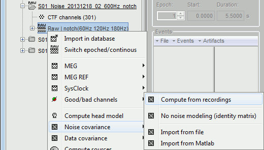
Select the menu Noise covariance > Compute from recordings. Available options:
Files: The top part of this window shows a summary of the files that have been selected to estimate the noise: 1 file of 120s at 600Hz. Total number of time samples in selected file: 72,000. We can also choose to use only a portion of this file, with the option "baseline". The large continuous files are split in blocks of a maximum of 10,000 samples that are then processed as different files.
Remove DC offset: All the selected blocks of data are baseline corrected and concatenated to form a large matrix "F". There are two options for baseline correction:
Block by block: The average value of each channel is subtracted from each block before concatenating files together.
Let Fi contain data from block #i: F = Concatenate[Fi - mean(Fi)].
Global: The average value of each channel is removed after concatenation (same correction for all blocks).
F = Concatenate[Fi] - mean(Concatenate[Fi]).The sample noise covariance is computed from F: NoiseCov = F * F' / Nsamples
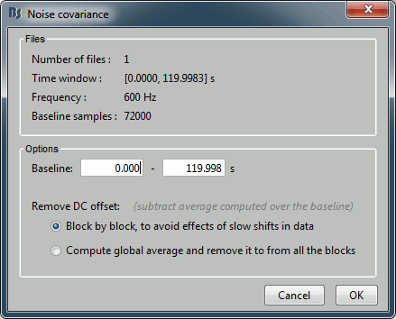
For this tutorial, keep the default options and click on [OK].
- One new file is created and appears under the noise data folder, next to the channel file. The corresponding contextual menus are:
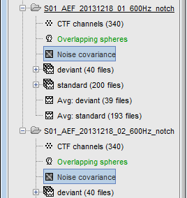
Display as image: Opens a display of the noise covariance matrix as an indexed image (same as double-click on file). This can be useful to quickly control the quality of the recordings: for instance, noisier channels appear as rows/columns marked in red.
Copy to other conditions: Copy the file obtained to all the other folders of the same subject, to avoid re-computing the noise covariance statistics again for each folder from the same session.
Copy to other subjects: Copy this file to all the folders of all the subjects in the protocol.
You can also copy a noise covariance file to another folder just like any other file:
Right-click > File > Copy/Paste, or keyboard shortcuts Ctrl+C/Ctrl+V.
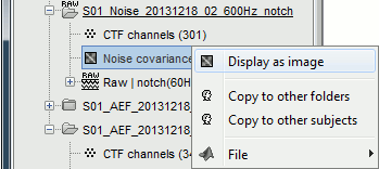
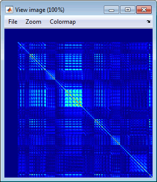
Right-click on the the noise covariance file > Copy to other folders: We need this file in the two folders where the epochs were imported before we compute the respective source models.
Variations on how to estimate sample noise covariance
The sample noise covariance matrix is straightforward to otbain. Brainstorm's interface features a lot of flexibility to select the files and time windows used to calculate the sample statistics. You need to have a clear understanding of the concept of "noise" to pick the best possible option. We support the notion that noise covariance accounts for contaminants that remain present in the data after pre-processing is complete. Hence it is not meant to account for eye blinks, heartbeats, muscle artifacts, flat or bad channels and noisy segments: all these the above need to be taken care of during previous preprocessing steps, as show in previous tutorial sections. The noise covariance entry is to account for remaining and stationnary instrumental, sensor and environmental noise components. For this reason, the ideal scenario is to use segments of recordings that contain exclusively this type of contaminant, or segments of recordings deemed not to contain any of brain signals of interest. This section is advanced reading material that can be used as a reference in a different experimental context.
The case of MEG
Empty room: actual noise measurements (due to the instrument, environment) using empty-room conditions (no subject under the MEG helmet) are possible in MEG. We recommend you obtain 2 to more minutes of empty-room data right before bringing the subject in the MEG room, or right after the experiment is finished. .
You can verify quatitatively how stable and reproducible is the noise covariance estimated (e.g., during the day/week). You may be in a "quiet environment" allowing that you re-use the same noise recordings and therfore, noise covariance matrix, for all runs and subjects acquired on the same day.
Resting baseline: Alternatively, when studying evoked responses (aka event-related responses), you can use a few minutes of recordings where the subject is resting, ie. not performing the task. Record those resting segments before or after the experiment, or before/after each run. This approach considers the resting brain activity as "noise", the sources estimated for the evoked response are going to be preferentially the ones that were not activated during the resting period.
Pre-stimulation baseline: It can also be a valid approach to use the pre-stimulation baseline of the individual trials to estimate the noise covariance. But keep in mind that in this case, everything in your pre-stimulation baseline is going to be attenuated in the source reconstruction, noise and brain activity. Therefore, your stimuli have to be distant enough in time so that the response to a stimulus is not recorded in the "baseline" of the following one. For repetitive stimuli, randomized delays between stimuli can help avoiding expectation effects in the baseline.
EEG
The EEG case is typically more complicated. It is not possible to estimate the noise of the sensors only. Only the two other approaches described for the MEG are still valid:
resting baseline and pre-stimulation baseline.
The noise level of the electrode recordings depends primarily on the quality of the connection with the skin, which varies a lot from a subject to another, or even during the acquisition of one single subject. The conductive gel or solution used on the electrodes tends to dry, and the electrode cap can move. Therefore, it is very important to use one channel file per subject, hence one noise covariance per subject. In some specific cases, if the quality of the recordings varies a lot over the time, it can be interesting to split long recordings in different runs, with different noise covariance matrices too.
EEG and resting state
When studying the resting brain, you cannot use resting recordings as a noise baseline. For MEG the best choice is to use empty room measurements. For EEG, you can chose between two different approaches: using the sensors variance, or not using any noise information.
Option #1: Calculate the covariance over a long segment of the resting recordings, but save only the diagonal, ie. the variance of the sensors. This option is available in the advanced options of the source computation: select the option "Diagonal noise covariance".
Option #2: Select "No noise modeling" in the popup menu. This would use an identity matrix instead of a noise covariance matrix (equal, unit variance of noise on every sensor). In the inverse modeling, this is equivalent to the assumption that the noise in the recordings is homoskedastic, and equivalent for all the sensors. The problem with this approach is that an electrode with a higher level of noise is going to be interpreted as a lot of activity in its region of the brain.
Noise and epilepsy
Analyzing a single interictal spike, using either EEG and MEG data, we are faced with a similar problem in defining what is noise. Even the brain activity before and after the spike can be very informative about the spike's generation, particularly if it is part of a sequence of interictal activity that precedes ictal (seizure) onset. Defining a segment of time adjacent the spike as "background" may not be practical. In practice, however, we can often find a period of time of spontaneous brain activity in the recordings that appears adequate for declaring as background, even in the epileptic patient. As discussed above, MEG has the additional option of using empty room data as a baseline, an option not available in EEG.
We thus have the same options as above:
Option #1a: Compute the noise covariance statistics from blocks of recordings away from the peak of any identified interictal spike, and keep only the diagonal (the variance of the sensors).
Option #1b: If a large period of time is available, calculate the full noise covariance.
Option #2(MEG): Use empty room data as the baseline.
Option #3: Select "No noise modeling" in the popup menu (identity matrix, unit variance of noise on every sensor).
Recommendations
Long noise recordings: In order to get a good estimation of the noise covariance, we need a significant number of time samples, at least N*(N+1)/2, where N is the number of sensors. This means about 40s for CTF275 recordings at 1000Hz, or 20s for 128-channel EEG at 500Hz. Always try to use as much data as possible for estimating this noise covariance.
Do not import averages: For this reason, you should never compute the noise covariance matrix from averaged responses. If you want to import recordings that you have fully pre-processed with another program, we recommend you import the individual trials and use them to compute the noise covariance. If you can only import the averaged responses in the Brainstorm database, you have to be aware that you may get poor results in the source estimation.
Using one block: If you want to use a segment of "quiet" recordings in a continuous file: right-click on the continuous file > Noise covariance > Compute from recordings, then copy the noise covariance to the other folders. This is the case described in this tutorial.
Use single trials: If you want to use the pre-stimulation baseline of the single trials, first import the trials in the database, then select all the groups of imported trials at once, right-click on one of them > Noise covariance > Compute from recordings, and finally copy the file to the other folders.
Using multiple continuous blocks: This is similar to the single trial case. Import in the database all the blocks you consider as quiet resting baselines, then select all the imported blocks in the database explorer > Noise covariance > Compute from recordings.
Data covariance
The beamforming approach to source localization requires a data covariance in input. The computation of a data covariance matrix is very similar to a noise covariance matrix, except that you need to target the segments of recordings of interest instead of the noise. In the case of an event-related study, you can consider all the recordings in a range of latencies after the stimulation corresponding to the effect you want to localize in the brain.
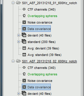
For run#01, select all the trials, right-click > Data covariance > Compute from recordings.
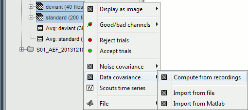
We need to specify two time windows from these recordings:
Baseline: Pre-stimulus time, used for DC offset correction (subtracts the baseline mean).
Data: Time segment of interest (let's use all the time available post-stimulus).
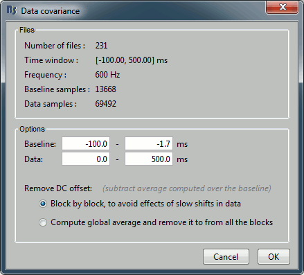
Repeat the operation for run#02.
On the hard drive
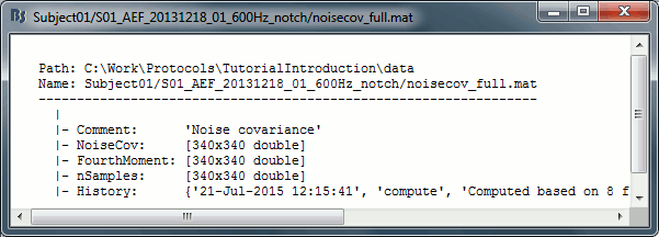
Right-click on any noise covariance file > File > View file contents:
Structure of the noise/data covariance files: noisecov_*.mat / ndatacov_*.mat
Comment: String displayed in the database explorer to represent this file.
NoiseCov: [nChannels x nChannels] noise covariance: F * F' ./ (nSamples-1)
Unknown values are set to zero.FourthMoment: [nChannels x nChannels] fourth order moments: F.^2 * F'.^2 ./ (nSamples-1)
nSamples: [nChannels x nChannels] number of time samples that were used for each pair of sensors. This is not necessarily the same value everywhere, some channels can be bad only for a few trials.
Related functions
process_noisecov.m: Function for process "Sources > Compute covariance (noise or data)"
bst_noisecov.m: Computes the data/noise covariance matrices.
panel_noisecov.m: Options panel.
Additional documentation
Forum: EEG reference: http://neuroimage.usc.edu/forums/showthread.php?1525#post6718

