|
Size: 2323
Comment:
|
Size: 2915
Comment:
|
| Deletions are marked like this. | Additions are marked like this. |
| Line 1: | Line 1: |
| = CTF electric phantom = | = MEG current phantom (CTF) = |
| Line 31: | Line 31: |
| * Right-click on the subject folder > '''Review raw file'''. <<BR>>Select the file format: "'''MEG/EEG: CTF (*.ds)'''" <<BR>>Select all the folders in: '''Sub01/MEEG'''. <<BR>><<BR>> {{attachment:phantom_review.gif||height="197",width="512"}} * The recordings were acquired on different days, the position of the phantom in the MEG helmet is not the same for the two runs. Left = noise (2015-06-03), Right = clean (2015-07-09)<<BR>><<BR>> {{attachment:phantom_registration.gif}} |
* Right-click on the subject folder > '''Review raw file'''. <<BR>>Select the file format: "'''MEG/EEG: CTF (*.ds)'''" <<BR>>Select all the folders in: '''sample_phantom'''. <<BR>><<BR>> {{attachment:phantom_review.gif||height="197",width="512"}} * Each folder corresponds to one dataset: * '''emptyroom_20150709_01.ds''': Phantom inside the MEG helmet, but not plugged in * '''phantom_20uA_20150603_03.ds''': Phantom active, 23Hz, 20uA, [0,-1.8,4.9]cm * '''phantom_200uA_20150709_01.ds''': Phantom active, 7Hz, 200uA, [0,-1.8,4.9]cm * The recordings were acquired on different days, the position of the phantom in the MEG helmet is not the same for the two runs. Left = 20uA, Right = 200uA<<BR>><<BR>> {{attachment:phantom_registration.gif||height="189",width="417"}} * For each of the three runs: right-click on "Link to raw file" > '''Switch epoched/continuous''' <<BR>><<BR>> {{attachment:phantom_continuous.gif||height="167",width="279"}} |
| Line 34: | Line 39: |
| == Import recordings == == Noise covariance == == Source modeling == == Dipole fitting with FieldTrip == |
MEG current phantom (CTF)
Authors: Francois Tadel, Elizabeth Bock
This tutorial explains how to use recordings from the CTF electric phantom to test dipole fitting functions.
Contents
Phantom description
[TODO] Pictures
[TODO] Nature of the dipole that is generated
[TODO] References
Download and installation
Requirements: You have already followed all the introduction tutorials and you have a working copy of Brainstorm installed on your computer.
Go to the Download page of this website, and download the file: sample_phantom.zip
- Unzip it in a folder that is not in any of the Brainstorm folders (program folder or database folder)
- Start Brainstorm (Matlab scripts or stand-alone version)
Select the menu File > Create new protocol. Name it "TutorialPhantom" and select the options:
"No, use individual anatomy",
"No, use one channel file per acquisition run (MEG)".
Generate anatomy
In the Matlab command window: type "generate_ctf_phantom".
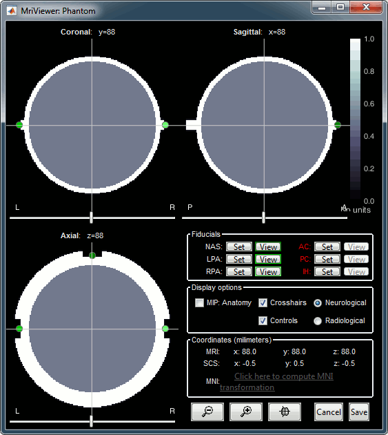
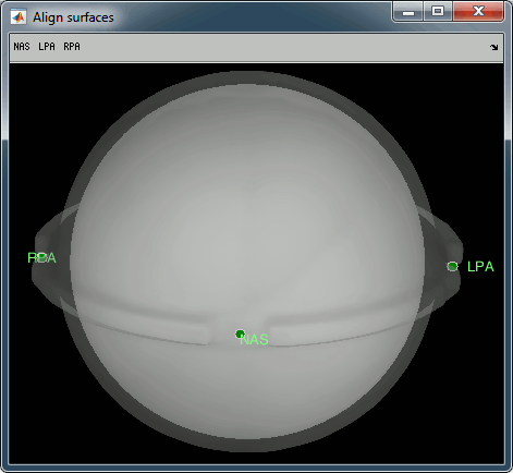
This creates a new subject Phantom and generates the "anatomy" for this device: one volume and a few surfaces representing the geometry of the phantom.
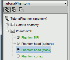
You can display the MRI and surfaces as presented in the introduction tutorials.
Access the recordings
- Switch to the "functional data" view.
Right-click on the subject folder > Review raw file.
Select the file format: "MEG/EEG: CTF (*.ds)"
Select all the folders in: sample_phantom.
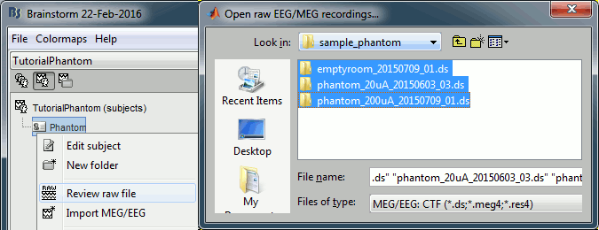
- Each folder corresponds to one dataset:
emptyroom_20150709_01.ds: Phantom inside the MEG helmet, but not plugged in
phantom_20uA_20150603_03.ds: Phantom active, 23Hz, 20uA, [0,-1.8,4.9]cm
phantom_200uA_20150709_01.ds: Phantom active, 7Hz, 200uA, [0,-1.8,4.9]cm
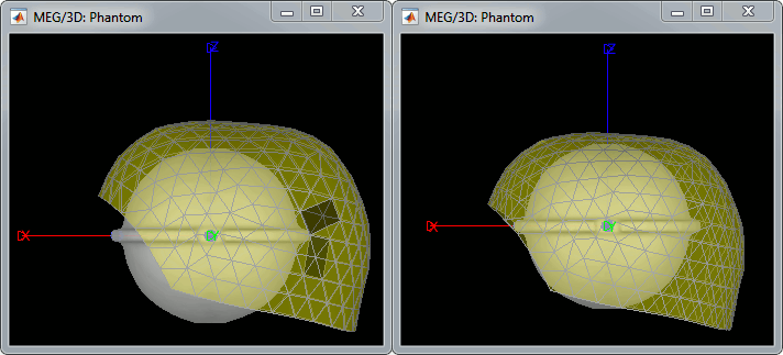
The recordings were acquired on different days, the position of the phantom in the MEG helmet is not the same for the two runs. Left = 20uA, Right = 200uA
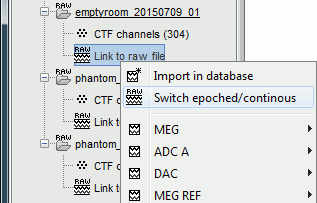
For each of the three runs: right-click on "Link to raw file" > Switch epoched/continuous
Import recordings
Noise covariance
Source modeling
Dipole fitting with FieldTrip
Scripting
Generate Matlab script
Available in the Brainstorm distribution: brainstorm3/toolbox/script/tutorial_phantom.m
