|
Size: 6406
Comment:
|
Size: 13284
Comment:
|
| Deletions are marked like this. | Additions are marked like this. |
| Line 1: | Line 1: |
| = Tutorial 20: Advanced scripting = | = Tutorial 28: Advanced scripting = '''[TUTORIAL UNDER DEVELOPMENT: NOT READY FOR PUBLIC USE] ''' |
| Line 4: | Line 6: |
| This tutorial explains how to use the Brainstorm scripting interface to run a full analysis, from the raw recordings to the source reconstruction. It is based on a median nerve stimulation experiment recorded at the Montreal Neurological Institute in 2011 with a CTF MEG 275 system. The sample dataset contains 6 minutes of recordings at 1200Hz for one subject and includes 100 stimulations of each arm. The tutorial follows the analysis steps detailed in the three advanced tutorials in the category [[http://neuroimage.usc.edu/brainstorm/Tutorials|Processing continuous recordings]]. You should read them before reading this tutorial, to have the explanations that go with the analysis steps. |
|
| Line 6: | Line 12: |
| = From CTF = The main window includes a graphical batching interface that directly benefits from the database explorer: files are organized as a tree of subjects and conditions, and simple drag-and-drop operations readily select files for subsequent batch processing. Most of the Brainstorm features are available through this interface, including pre-processing of the recordings, averaging, time-frequency decompositions, and computing statistics. A full analysis pipeline can be created in a few minutes, saved in the user’s preferences and reloaded in one click, executed directly or exported as a Matlab script. The available processes are organized in a plug-in structure. Any Matlab script that is added to the plug-in folder (brainstorm3/toolbox/process/functions/) and has the right format will be automatically detected and made available in the GUI. This mechanism makes the contribution from other developers to Brainstorm very easy. == Creating a pipeline == === List of processes === 1. Click on Run. The Process selection window appears, with which you can create an analysis pipeline (ie. a list of process that are applied on the selected files one after the other). The first button in the toolbar shows the list of processed that are currently available. If you click on a menu, it's added to the list. {{http://neuroimage.usc.edu/brainstorm/Tutorials/TutProcesses?action=AttachFile&do=get&target=pipeline1.gif|pipeline1.gif|class="attachment"}} 1. Some menus appear in grey (example: Sources > Spatial smoothing). This means that they are not meant to be applied to the type of data that you have in input, or at the end of the current pipeline. The "spatial smoothing" process may only be run on source files. 1. When you select a process, a list of options specific to this process is shown in the window. * To delete a process: Select it and press the ''Delete'' key, or the big cross in the toolbar. * With the "up arrow" and "down arrow" buttons in the toolbar, you can move up/down a process in the pipeline. 1. Now add the following processes, and set their options: * '''Pre-process > Band-pass filter''': 2Hz - 30Hz * In some processes, you can specify the type(s) of sensors on which you want to apply the process. This way you can for instance apply different filters on the EEG and the MEG, if you have both in the same files. * '''Extract > Extract time''': 40.00ms - 49.60ms, overwrite initial file * This will extract from each file a small time window around the main response peak. * Selecting the overwrite option will replace the previous file (bandpass), with the output of this process (bandpass+extract). This option is usually unselected for the first process in the list, then selected automatically. * '''Average > Average over time''': Overwrite initial file * Compute the average over this small time window. {{http://neuroimage.usc.edu/brainstorm/Tutorials/TutProcesses?action=AttachFile&do=get&target=pipeline2.gif|pipeline2.gif|class="attachment"}} 1. Save your pipeline: Click on the last button in the toolbar > Save > New... > Type "process_avg45". === Saving/exporting a pipeline === The last button in the the toolbar offers a list of menus to save, load and export the pipelines. . {{http://neuroimage.usc.edu/brainstorm/Tutorials/TutProcesses?action=AttachFile&do=get&target=pipeline3.gif|pipeline3.gif|class="attachment"}} * '''Load''': List of processes that are saved in the user preferences * '''Load from file''': Import a pipeline from a pipeline_...mat file (previously saved with the menu "Save as Matlab matrix") * '''Save''': Save the pipeline in the user preferences, to be able to access it really fast after * '''Save as Matlab matrix''': Exports the pipeline for a Matlab structure in a .mat file. Allows different users to exchange their analysis pipelines (or a single user between different computers). * '''Generate .m script''': This option generates a human-readable Matlab script that can be re-used for other purposes or modified. * '''Delete''': Remove a pipeline that is saved in the user preferences. * '''Reset options''': Brainstorm saves automatically for each user the options of all the processes. This menu removes all the saved options, and set them back to the default values. Here is the Matlab script that is generated automatically for this pipeline. . {{http://neuroimage.usc.edu/brainstorm/Tutorials/TutProcesses?action=AttachFile&do=get&target=script.gif|script.gif|class="attachment"}} . Click on Ok, in the pipeline window. After a few seconds, you will see two new files in the database, and the "Report viewer" window. === Report viewer === Each time the pipeline editor is used to executed to run a list of processes, a report is generated and saved in the user home folder (/home/username/reports/). The report viewer shows as an HTML page some of the information saved in this report structure: the date and duration of execution, the list of processes, the input and output files. It reports all the warning and errors that happen during the execution. The report viewer does not necessarily appear automatically at the end of the last process: it is shown only when more than one processes were executed, or when any of the processes returned an error or a warning. When running processes manually from a script, the calls bst_report(Start, Save, Open) explicitly indicate when the logging of the events should start and stop. You can add images to the reports for quality control using the process "File > Save snapshot". {{http://neuroimage.usc.edu/brainstorm/Tutorials/TutProcesses?action=AttachFile&do=get&target=report.gif|output.gif|class="attachment"}} After you close the report window, you can re-open the last report with the main menu of the Brainstorm window: '''File > Report viewer'''. With the buttons in the toolbar, you can go back to the previous reports saved from the same protocol. <<EmbedContent("http://neuroimage.usc.edu/bst/get_prevnext.php?prev=Tutorials/Connectivity")>> |
== Script generation == == Script edition == - Add loops, load files, ... Loops: http://neuroimage.usc.edu/forums/showthread.php?2429-Problem-using-tags == File manipulation == * Modify a structure manually: Export to Matlab/Import from Matlab * File manipulation: file_short, file_fullpath, in_bst_*... * Documentation of all file structures: point at the appropriate tutorials * Select files from the database (with bst_get and processes) == Creating the analysis pipeline == Select the menu File > Create new protocol. Name it "'''TutorialScript'''" and select the options: * "'''No, use individual anatomy'''", * "'''Yes, use one channel file per subject'''". To start building your analysis pipeline, just click on the "'''Run'''" button in the Process1 tab. We don't need any file in input, as we are going to select the files to import in the script itself. Then add all the processes listed below. The output of each process is the input of the following one, this is why the order of the processes is important. === Import anatomy > Import anatomy folder === * Folder to import: sample_raw/Anatomy File format: "FreeSurfer folder" * Fiducials: Copy what is indicated below. This is a reason it is usually easier to do this step in interactive mode, and then run only the script starting from the next step. * Input: None; Output: None {{http://neuroimage.usc.edu/brainstorm/Tutorials/TutRawScript?action=AttachFile&do=get&target=process_import_freesurfer.gif|process_import_freesurfer.gif|class="attachment"}} === Import recordings > Create link to raw file === * File to import: Select the folder sample_raw/Data/subj001_somatosensory_20111109_01_AUX-f.ds * Input: None; Output: Raw file {{http://neuroimage.usc.edu/brainstorm/Tutorials/TutRawScript?action=AttachFile&do=get&target=process_import_data_raw.gif|process_import_data_raw.gif|class="attachment"}} === Pre-process > Notch filter === Input: Raw file ; Output: Raw file (new) {{http://neuroimage.usc.edu/brainstorm/Tutorials/TutRawScript?action=AttachFile&do=get&target=process_sin_remove.gif|process_sin_remove.gif|class="attachment"}} === Events > Detect eye blinks === Input: Raw file ; Output: Raw file {{http://neuroimage.usc.edu/brainstorm/Tutorials/TutRawScript?action=AttachFile&do=get&target=process_evt_detect_eog.gif|process_evt_detect_eog.gif|class="attachment"}} === Events > Compute SSP: eye blinks === Input: Raw file ; Output: Raw file {{http://neuroimage.usc.edu/brainstorm/Tutorials/TutRawScript?action=AttachFile&do=get&target=process_ssp_eog.gif|process_ssp_eog.gif|class="attachment"}} === Import recordings > Import MEG/EEG : Events === Input: Raw file ; Output: 199 epochs in 2 conditions {{http://neuroimage.usc.edu/brainstorm/Tutorials/TutRawScript?action=AttachFile&do=get&target=process_import_data_event.gif|process_import_data_event.gif|class="attachment"}} === Pre-process > Remove DC offset === Input: 199 epochs ; Output: 199 epochs {{http://neuroimage.usc.edu/brainstorm/Tutorials/TutRawScript?action=AttachFile&do=get&target=process_baseline.gif|process_baseline.gif|class="attachment"}} === Pre-process > Add time offset === Input: 199 epochs ; Output: 199 epochs {{http://neuroimage.usc.edu/brainstorm/Tutorials/TutRawScript?action=AttachFile&do=get&target=process_timeoffset.gif|process_timeoffset.gif|class="attachment"}} === Sources > Compute noise covariance === Since the epochs are currently selected and pre-processed: we can use them to estimate the noise covariance matrix before we move on with the calculation of the average. Input: 199 epochs ; Output: 199 epochs {{http://neuroimage.usc.edu/brainstorm/Tutorials/TutRawScript?action=AttachFile&do=get&target=process_noisecov.gif|process_noisecov.gif|class="attachment"}} === Average > Average files === Input: 199 epochs ; Output: 2 averages {{http://neuroimage.usc.edu/brainstorm/Tutorials/TutRawScript?action=AttachFile&do=get&target=process_average.gif|process_average.gif|class="attachment"}} === File > Save snapshot: Sensors/MRI registration === Input: 2 averages ; Output: 2 averages {{http://neuroimage.usc.edu/brainstorm/Tutorials/TutRawScript?action=AttachFile&do=get&target=process_snapshot.gif|process_snapshot.gif|class="attachment"}} === File > Save snapshot: Recordings time series === Input: 2 averages ; Output: 2 averages {{http://neuroimage.usc.edu/brainstorm/Tutorials/TutRawScript?action=AttachFile&do=get&target=process_snapshot2.gif|process_snapshot2.gif|class="attachment"}} === Sources > Compute head model === Input: 2 averages ; Output: 2 averages {{http://neuroimage.usc.edu/brainstorm/Tutorials/TutRawScript?action=AttachFile&do=get&target=process_headmodel.gif|process_headmodel.gif|class="attachment"}} === Sources > Compute sources === Input: 2 averages ; Output: all the source files (1 raw + 2 average + 199 epochs = 202 files) {{http://neuroimage.usc.edu/brainstorm/Tutorials/TutRawScript?action=AttachFile&do=get&target=process_inverse.gif|process_inverse.gif|class="attachment"}} == Save the pipeline == === Save in current workspace === Use the menus on top of the pipeline editor to save this list of processes on your computer. The menu "Save > New..." will create an entry readily available in your Brainstorm installation in the Load section of the same menu. {{http://neuroimage.usc.edu/brainstorm/Tutorials/TutRawScript?action=AttachFile&do=get&target=savePipeline.gif|savePipeline.gif|class="attachment"}} === Export as script === Use the menu "Generate .m script" to create a Matlab script that would have the exact same result as running this analysis pipeline from the Brainstorm interface. This script is also available in the Brainstorm distribution: '''brainstorm3/toolbox/script/tutorial_raw.m ''' {{{ % Script generated by Brainstorm v3.2 (22-Jul-2014) % Input files sFiles = []; SubjectNames = {... 'Subject01'}; RawFiles = {... 'C:\Work\RawData\Tutorials\sample_raw\Anatomy', ... 'C:\Work\RawData\Tutorials\sample_raw\Data\subj001_somatosensory_20111109_01_AUX-f.ds'}; % Start a new report bst_report('Start', sFiles); % Process: Import anatomy folder sFiles = bst_process('CallProcess', 'process_import_anatomy', ... sFiles, [], ... 'subjectname', SubjectNames{1}, ... 'mrifile', {RawFiles{1}, 'FreeSurfer'}, ... 'nvertices', 15000, ... 'nas', [127, 212, 123], ... 'lpa', [55, 124, 119], ... 'rpa', [200, 129, 114], ... 'ac', [129, 137, 157], ... 'pc', [129, 113, 157], ... 'ih', [129, 118, 209]); % Process: Create link to raw file sFiles = bst_process('CallProcess', 'process_import_data_raw', ... sFiles, [], ... 'subjectname', SubjectNames{1}, ... 'datafile', {RawFiles{2}, 'CTF'}, ... 'channelreplace', 1, ... 'channelalign', 1); % Process: Notch filter: 60Hz 120Hz 180Hz sFiles = bst_process('CallProcess', 'process_notch', ... sFiles, [], ... 'freqlist', [60, 120, 180], ... 'sensortypes', 'MEG, EEG', ... 'read_all', 0); % Process: Detect eye blinks sFiles = bst_process('CallProcess', 'process_evt_detect_eog', ... sFiles, [], ... 'channelname', 'EEG058', ... 'timewindow', [], ... 'eventname', 'blink'); % Process: Detect heartbeats sFiles = bst_process('CallProcess', 'process_evt_detect_ecg', ... sFiles, [], ... 'channelname', 'EEG057', ... 'timewindow', [], ... 'eventname', 'cardiac'); % Process: SSP EOG: blink sFiles = bst_process('CallProcess', 'process_ssp_eog', ... sFiles, [], ... 'eventname', 'blink', ... 'sensortypes', 'MEG, EEG', ... 'usessp', 0); % Process: Import MEG/EEG: Events sFiles = bst_process('CallProcess', 'process_import_data_event', ... sFiles, [], ... 'subjectname', SubjectNames{1}, ... 'condition', '', ... 'eventname', 'left, right', ... 'timewindow', [], ... 'epochtime', [-0.1, 0.3], ... 'createcond', 1, ... 'ignoreshort', 1, ... 'usectfcomp', 1, ... 'usessp', 1, ... 'freq', [], ... 'baseline', [-0.1, -0.0008333333333]); % Process: Add time offset: -4.20ms sFiles = bst_process('CallProcess', 'process_timeoffset', ... sFiles, [], ... 'offset', -0.0042, ... 'overwrite', 1); % Process: Compute noise covariance sFiles = bst_process('CallProcess', 'process_noisecov', ... sFiles, [], ... 'baseline', [-0.1042, 0], ... 'dcoffset', 1, ... 'method', 1, ... % Full noise covariance matrix 'copycond', 0, ... 'copysubj', 0); % Process: Average: By condition (subject average) sFiles = bst_process('CallProcess', 'process_average', ... sFiles, [], ... 'avgtype', 3, ... 'avg_func', 1, ... % Arithmetic average: mean(x) 'keepevents', 0); % Process: Snapshot: Sensors/MRI registration sFiles = bst_process('CallProcess', 'process_snapshot', ... sFiles, [], ... 'target', 1, ... % Sensors/MRI registration 'modality', 1, ... % MEG (All) 'orient', 1, ... % left 'time', 0, ... 'contact_time', [0, 0.1], ... 'contact_nimage', 12, ... 'comment', 'MEG/MRI Registration'); % Process: Snapshot: Recordings time series sFiles = bst_process('CallProcess', 'process_snapshot', ... sFiles, [], ... 'target', 5, ... % Recordings time series 'modality', 1, ... % MEG (All) 'orient', 1, ... % left 'time', 0, ... 'contact_time', [0, 0.1], ... 'contact_nimage', 12, ... 'comment', 'Evoked response'); % Process: Compute head model sFiles = bst_process('CallProcess', 'process_headmodel', ... sFiles, [], ... 'comment', '', ... 'sourcespace', 1, ... 'meg', 3, ... % Overlapping spheres 'eeg', 3, ... % OpenMEEG BEM 'ecog', 2, ... % OpenMEEG BEM 'seeg', 2, ... 'openmeeg', struct(... 'BemFiles', {{}}, ... 'BemNames', {{'Scalp', 'Skull', 'Brain'}}, ... 'BemCond', [1, 0.0125, 1], ... 'BemSelect', [1, 1, 1], ... 'isAdjoint', 0, ... 'isAdaptative', 1, ... 'isSplit', 0, ... 'SplitLength', 4000)); % Process: Compute sources sFiles = bst_process('CallProcess', 'process_inverse', ... sFiles, [], ... 'comment', '', ... 'method', 1, ... % Minimum norm estimates (wMNE) 'wmne', struct(... 'NoiseCov', [], ... 'InverseMethod', 'wmne', ... 'ChannelTypes', {{}}, ... 'SNR', 3, ... 'diagnoise', 0, ... 'SourceOrient', {{'fixed'}}, ... 'loose', 0.2, ... 'depth', 1, ... 'weightexp', 0.5, ... 'weightlimit', 10, ... 'regnoise', 1, ... 'magreg', 0.1, ... 'gradreg', 0.1, ... 'eegreg', 0.1, ... 'ecogreg', 0.1, ... 'seegreg', 0.1, ... 'fMRI', [], ... 'fMRIthresh', [], ... 'fMRIoff', 0.1, ... 'pca', 1), ... 'sensortypes', 'MEG, MEG MAG, MEG GRAD, EEG', ... 'output', 1); % Kernel only: shared % Save and display report ReportFile = bst_report('Save', sFiles); bst_report('Open', ReportFile); }}} == Report viewer == Click on Run to start the script. As this process is taking screen captures, do not use your computer for something else at the same time: if another window covers the Brainstorm figures, it will not capture the right images. At the end, the report viewer is opened to show the status of all the processes, the information messages, the list of input and output files, and the screen captures. The report is saved in your home folder ($home/.brainstorm/reports). If you close this window, you can get it back with the menu File > Report viewer. {{http://neuroimage.usc.edu/brainstorm/Tutorials/TutRawScript?action=AttachFile&do=get&target=report1.gif|report1.gif|class="attachment"}} {{http://neuroimage.usc.edu/brainstorm/Tutorials/TutRawScript?action=AttachFile&do=get&target=report2.gif|report2.gif|class="attachment"}} <<EmbedContent("http://neuroimage.usc.edu/bst/get_prevnext.php?prev=Tutorials/Workflows")>> |
Tutorial 28: Advanced scripting
[TUTORIAL UNDER DEVELOPMENT: NOT READY FOR PUBLIC USE]
Authors: Francois Tadel, Elizabeth Bock, Sylvain Baillet
This tutorial explains how to use the Brainstorm scripting interface to run a full analysis, from the raw recordings to the source reconstruction. It is based on a median nerve stimulation experiment recorded at the Montreal Neurological Institute in 2011 with a CTF MEG 275 system. The sample dataset contains 6 minutes of recordings at 1200Hz for one subject and includes 100 stimulations of each arm.
The tutorial follows the analysis steps detailed in the three advanced tutorials in the category Processing continuous recordings. You should read them before reading this tutorial, to have the explanations that go with the analysis steps.
Contents
Script generation
Script edition
- Add loops, load files, ...
Loops: http://neuroimage.usc.edu/forums/showthread.php?2429-Problem-using-tags
File manipulation
- Modify a structure manually: Export to Matlab/Import from Matlab
- File manipulation: file_short, file_fullpath, in_bst_*...
- Documentation of all file structures: point at the appropriate tutorials
- Select files from the database (with bst_get and processes)
Creating the analysis pipeline
Select the menu File > Create new protocol. Name it "TutorialScript" and select the options:
"No, use individual anatomy",
"Yes, use one channel file per subject".
To start building your analysis pipeline, just click on the "Run" button in the Process1 tab. We don't need any file in input, as we are going to select the files to import in the script itself. Then add all the processes listed below. The output of each process is the input of the following one, this is why the order of the processes is important.
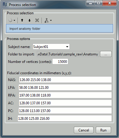
Import anatomy > Import anatomy folder
- Folder to import: sample_raw/Anatomy
File format: "FreeSurfer folder"
- Fiducials: Copy what is indicated below. This is a reason it is usually easier to do this step in interactive mode, and then run only the script starting from the next step.
- Input: None; Output: None
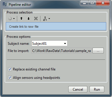
Import recordings > Create link to raw file
- File to import: Select the folder sample_raw/Data/subj001_somatosensory_20111109_01_AUX-f.ds
- Input: None; Output: Raw file
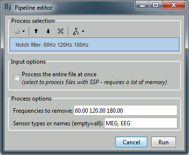
Pre-process > Notch filter
Input: Raw file ; Output: Raw file (new)
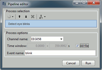
Events > Detect eye blinks
Input: Raw file ; Output: Raw file
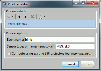
Events > Compute SSP: eye blinks
Input: Raw file ; Output: Raw file
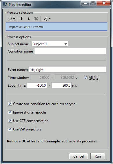
Import recordings > Import MEG/EEG : Events
Input: Raw file ; Output: 199 epochs in 2 conditions
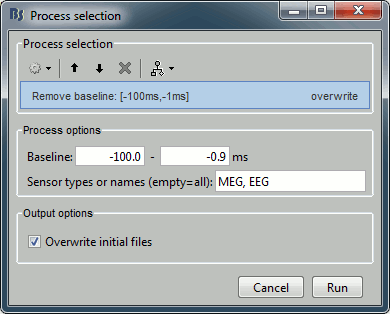
Pre-process > Remove DC offset
Input: 199 epochs ; Output: 199 epochs
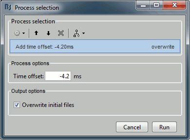
Pre-process > Add time offset
Input: 199 epochs ; Output: 199 epochs
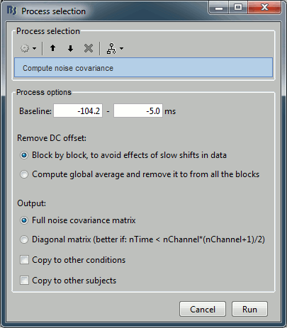
Sources > Compute noise covariance
Since the epochs are currently selected and pre-processed: we can use them to estimate the noise covariance matrix before we move on with the calculation of the average.
Input: 199 epochs ; Output: 199 epochs
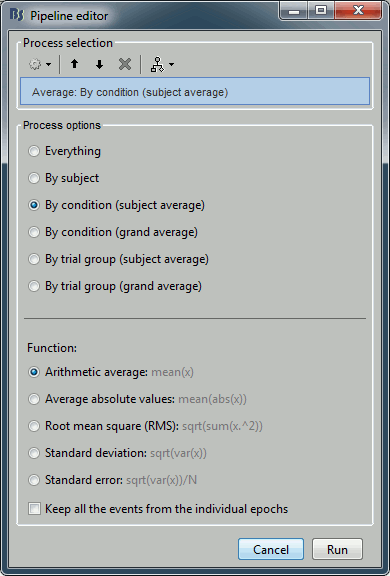
Average > Average files
Input: 199 epochs ; Output: 2 averages
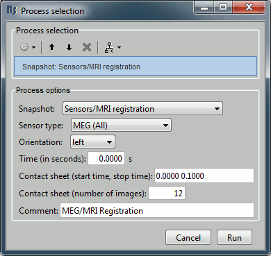
File > Save snapshot: Sensors/MRI registration
Input: 2 averages ; Output: 2 averages
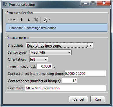
File > Save snapshot: Recordings time series
Input: 2 averages ; Output: 2 averages
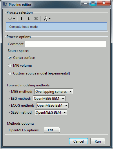
Sources > Compute head model
Input: 2 averages ; Output: 2 averages
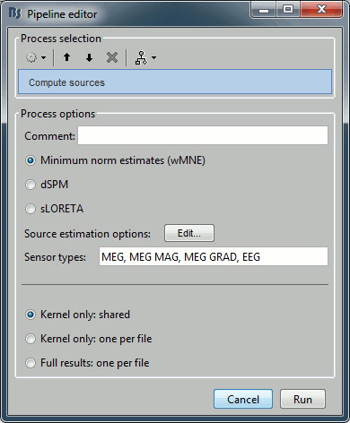
Sources > Compute sources
Input: 2 averages ; Output: all the source files (1 raw + 2 average + 199 epochs = 202 files)
Save the pipeline
Save in current workspace
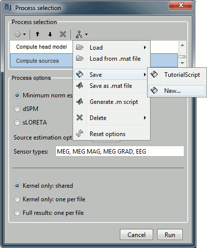
Use the menus on top of the pipeline editor to save this list of processes on your computer. The menu "Save > New..." will create an entry readily available in your Brainstorm installation in the Load section of the same menu.
Export as script
Use the menu "Generate .m script" to create a Matlab script that would have the exact same result as running this analysis pipeline from the Brainstorm interface.
This script is also available in the Brainstorm distribution: brainstorm3/toolbox/script/tutorial_raw.m
% Script generated by Brainstorm v3.2 (22-Jul-2014)

% Input files
sFiles = [];
SubjectNames = {...
    'Subject01'};
RawFiles = {...
    'C:\Work\RawData\Tutorials\sample_raw\Anatomy', ...
    'C:\Work\RawData\Tutorials\sample_raw\Data\subj001_somatosensory_20111109_01_AUX-f.ds'};

% Start a new report
bst_report('Start', sFiles);

% Process: Import anatomy folder
sFiles = bst_process('CallProcess', 'process_import_anatomy', ...
    sFiles, [], ...
    'subjectname', SubjectNames{1}, ...
    'mrifile', {RawFiles{1}, 'FreeSurfer'}, ...
    'nvertices', 15000, ...
    'nas', [127, 212, 123], ...
    'lpa', [55, 124, 119], ...
    'rpa', [200, 129, 114], ...
    'ac', [129, 137, 157], ...
    'pc', [129, 113, 157], ...
    'ih', [129, 118, 209]);

% Process: Create link to raw file
sFiles = bst_process('CallProcess', 'process_import_data_raw', ...
    sFiles, [], ...
    'subjectname', SubjectNames{1}, ...
    'datafile', {RawFiles{2}, 'CTF'}, ...
    'channelreplace', 1, ...
    'channelalign', 1);

% Process: Notch filter: 60Hz 120Hz 180Hz
sFiles = bst_process('CallProcess', 'process_notch', ...
    sFiles, [], ...
    'freqlist', [60, 120, 180], ...
    'sensortypes', 'MEG, EEG', ...
    'read_all', 0);

% Process: Detect eye blinks
sFiles = bst_process('CallProcess', 'process_evt_detect_eog', ...
    sFiles, [], ...
    'channelname', 'EEG058', ...
    'timewindow', [], ...
    'eventname', 'blink');

% Process: Detect heartbeats
sFiles = bst_process('CallProcess', 'process_evt_detect_ecg', ...
    sFiles, [], ...
    'channelname', 'EEG057', ...
    'timewindow', [], ...
    'eventname', 'cardiac');

% Process: SSP EOG: blink
sFiles = bst_process('CallProcess', 'process_ssp_eog', ...
    sFiles, [], ...
    'eventname', 'blink', ...
    'sensortypes', 'MEG, EEG', ...
    'usessp', 0);

% Process: Import MEG/EEG: Events
sFiles = bst_process('CallProcess', 'process_import_data_event', ...
    sFiles, [], ...
    'subjectname', SubjectNames{1}, ...
    'condition', '', ...
    'eventname', 'left, right', ...
    'timewindow', [], ...
    'epochtime', [-0.1, 0.3], ...
    'createcond', 1, ...
    'ignoreshort', 1, ...
    'usectfcomp', 1, ...
    'usessp', 1, ...
    'freq', [], ...
    'baseline', [-0.1, -0.0008333333333]);

% Process: Add time offset: -4.20ms
sFiles = bst_process('CallProcess', 'process_timeoffset', ...
    sFiles, [], ...
    'offset', -0.0042, ...
    'overwrite', 1);

% Process: Compute noise covariance
sFiles = bst_process('CallProcess', 'process_noisecov', ...
    sFiles, [], ...
    'baseline', [-0.1042, 0], ...
    'dcoffset', 1, ...
    'method', 1, ...  % Full noise covariance matrix
    'copycond', 0, ...
    'copysubj', 0);

% Process: Average: By condition (subject average)
sFiles = bst_process('CallProcess', 'process_average', ...
    sFiles, [], ...
    'avgtype', 3, ...
    'avg_func', 1, ...  % Arithmetic average: mean(x)
    'keepevents', 0);

% Process: Snapshot: Sensors/MRI registration
sFiles = bst_process('CallProcess', 'process_snapshot', ...
    sFiles, [], ...
    'target', 1, ...  % Sensors/MRI registration
    'modality', 1, ...  % MEG (All)
    'orient', 1, ...  % left
    'time', 0, ...
    'contact_time', [0, 0.1], ...
    'contact_nimage', 12, ...
    'comment', 'MEG/MRI Registration');

% Process: Snapshot: Recordings time series
sFiles = bst_process('CallProcess', 'process_snapshot', ...
    sFiles, [], ...
    'target', 5, ...  % Recordings time series
    'modality', 1, ...  % MEG (All)
    'orient', 1, ...  % left
    'time', 0, ...
    'contact_time', [0, 0.1], ...
    'contact_nimage', 12, ...
    'comment', 'Evoked response');

% Process: Compute head model
sFiles = bst_process('CallProcess', 'process_headmodel', ...
    sFiles, [], ...
    'comment', '', ...
    'sourcespace', 1, ...
    'meg', 3, ...  % Overlapping spheres
    'eeg', 3, ...  % OpenMEEG BEM
    'ecog', 2, ...  % OpenMEEG BEM
    'seeg', 2, ...
    'openmeeg', struct(...
         'BemFiles', {{}}, ...
         'BemNames', {{'Scalp', 'Skull', 'Brain'}}, ...
         'BemCond', [1, 0.0125, 1], ...
         'BemSelect', [1, 1, 1], ...
         'isAdjoint', 0, ...
         'isAdaptative', 1, ...
         'isSplit', 0, ...
         'SplitLength', 4000));

% Process: Compute sources
sFiles = bst_process('CallProcess', 'process_inverse', ...
    sFiles, [], ...
    'comment', '', ...
    'method', 1, ...  % Minimum norm estimates (wMNE)
    'wmne', struct(...
         'NoiseCov', [], ...
         'InverseMethod', 'wmne', ...
         'ChannelTypes', {{}}, ...
         'SNR', 3, ...
         'diagnoise', 0, ...
         'SourceOrient', {{'fixed'}}, ...
         'loose', 0.2, ...
         'depth', 1, ...
         'weightexp', 0.5, ...
         'weightlimit', 10, ...
         'regnoise', 1, ...
         'magreg', 0.1, ...
         'gradreg', 0.1, ...
         'eegreg', 0.1, ...
         'ecogreg', 0.1, ...
         'seegreg', 0.1, ...
         'fMRI', [], ...
         'fMRIthresh', [], ...
         'fMRIoff', 0.1, ...
         'pca', 1), ...
    'sensortypes', 'MEG, MEG MAG, MEG GRAD, EEG', ...
    'output', 1);  % Kernel only: shared

% Save and display report
ReportFile = bst_report('Save', sFiles);
bst_report('Open', ReportFile);
Report viewer
Click on Run to start the script.
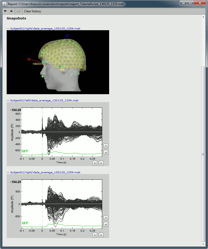
As this process is taking screen captures, do not use your computer for something else at the same time: if another window covers the Brainstorm figures, it will not capture the right images.
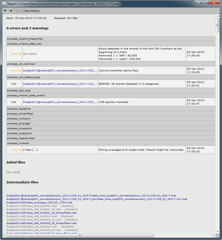
At the end, the report viewer is opened to show the status of all the processes, the information messages, the list of input and output files, and the screen captures. The report is saved in your home folder ($home/.brainstorm/reports). If you close this window, you can get it back with the menu File > Report viewer.
