|
Size: 28003
Comment:
|
Size: 36721
Comment:
|
| Deletions are marked like this. | Additions are marked like this. |
| Line 154: | Line 154: |
| == Interaction with Matlab == | == Evaluate in Matlab == |
| Line 199: | Line 199: |
| * '''File names''': Scripts and functions, only lower case, separation with "_" (eg. process_average) * '''Sub-functions''': Inside a .m file, name starting with a capital, camel-case (eg. CallProcess, Start). |
* '''File names''': Scripts and functions, only lower case, separation with "_" (eg. process_fft, bst_get). * '''Sub-functions''': Inside a .m file, name starting with a capital, CamelCase (eg. CallProcess, Start). |
| Line 258: | Line 258: |
| * Select process '''File > Select files: By tag''': Search="low", Search the comment, '''Ignore '''the files. <<BR>><<BR>>{{attachment:select_tag.gif}} | * Select process '''File > Select files: By tag''': Search="low", Search the comment, '''Ignore '''the files. <<BR>><<BR>> {{attachment:select_tag.gif||height="252",width="261"}} |
| Line 279: | Line 279: |
| {{attachment:add_tag.gif}} | . {{attachment:add_tag.gif||height="203",width="456"}} |
| Line 282: | Line 282: |
| . - gui / nogui - selecting protocol - delete existing protocol == Selecting files == - Inputs / outputs - Select processes - Adding tags to help with the file selection later |
Brainstorm must be running in the background for these scripts to run properly. The interface doesn't have to be visible on the screen, but the database engine must be running for processing requests. At the beginning of your script, you can explicitely start or restart Brainstorm. '''brainstorm''': Start Brainstorm with the regular GUI. '''brainstorm nogui''': Start in silent mode, without the GUI, without progress bar, without user interactions. If you want to start Brainstorm only if Brainstorm is not already running, you can use the following code: {{{ if ~brainstorm('status') brainstorm nogui end }}} To select a specific protocol at the beginning of your script: {{{ ProtocolName = 'TutorialIntroduction'; % Get the protocol index iProtocol = bst_get('Protocol', ProtocolName); if isempty(iProtocol) error(['Unknown protocol: ' ProtocolName]); end % Select the current procotol gui_brainstorm('SetCurrentProtocol', iProtocol); }}} To delete the protocol and start over: {{{ % Delete existing protocol gui_brainstorm('DeleteProtocol', ProtocolName); % Create new protocol gui_brainstorm('CreateProtocol', ProtocolName, 0, 0); }}} |
| Line 292: | Line 316: |
| bst_get / bst_set * '''iStudy''': Index of the study, get the structure with sStudy=bst_get('Study', sInput.iStudy) * '''iItem''': Index of file in its category (example for recordings: sStudy.Data(sInput.iItem)) sStudy = bst_get('Study', sAvgData(1).iStudy) sStudy.Data(sAvgData(1).iItem) == File manipulation == |
The functions '''bst_get''' and '''bst_set''' allow you to query the database, access the configuration of the software and some display parameters. The complete reference documentation of these functions is included directly in their code (brainstorm3/toolbox/core/bst_get.m and bst_set.m). Let's start with a few simple examples: {{{ >> ProtocolInfo = bst_get('ProtocolInfo') % Returns the configuration of the current protocol ProtocolInfo = Comment: 'TutorialIntroduction' STUDIES: 'C:\Work\Protocols\TutorialIntroduction\data' SUBJECTS: 'C:\Work\Protocols\TutorialIntroduction\anat' iStudy: 6 UseDefaultAnat: 0 UseDefaultChannel: 0 >> isGUI = bst_get('isGUI') % Is the Brainstorm interface currently displayed (0=no, 1=yes) >> bst_set('FlipYAxis', 1) % The new figures will have the Y axis flipped >> bst_set('TSDisplayMode', 'butterfly') % The new figures will use a "butterfly" view >> bst_set('FieldTripDir', FieldTripDir) % Set the path where the FieldTrip toolbox is installed }}} To reference the files in the database, each protocol is subdivided in '''Subjects''' (the "anat" folder and containing the MRI, surfaces and atlases) and '''Studies''' (the "data" folder, including the recordings, channel files and all the analyses). Each Study corresponds to a sub-folder (eg. protocol/data/subject01/run01/), and is attached to only one subject. Subjects and Studies are referenced in the protocol with a unique index most of the time kept in variables named '''iSubject''' and '''iStudy'''. The files available in them are also referenced with indices, with variables such as iAnatomy, iSurface, iData, iHeadModel, iResults, iTimefreq. You can see the indices in the database explorer by hovering your mouse over the nodes of the tree: {{attachment:db_indices.gif||height="64",width="715"}} Example: Getting the '''study structure''' from the variable sAvgData, defined in the script: {{{ >> sAvgData(1) ans = iStudy: 6 iItem: 1 ... >> sStudy = bst_get('Study', sAvgData(1).iStudy) % Get a study structure with its index sStudy = Name: 'S01_AEF_20131218_01_600Hz_notch' FileName: 'Subject01/S01_AEF_20131218_01_600Hz_notch/brainstormstudy.mat' DateOfStudy: '13-May-2016' BrainStormSubject: 'Subject01/brainstormsubject.mat' % Corresponding subject filename Condition: {'S01_AEF_20131218_01_600Hz_notch'} % Name of the condition (=folder) Channel: [1x1 struct] % Channel file for the folder iChannel: [] % Not used anymore Data: [1x242 struct] % List of "data" files in the folder HeadModel: [1x1 struct] % List of head models in the folder iHeadModel: 1 % Default head model (file in green) Result: [1x244 struct] % List of source files and source links Stat: [1x0 struct] % List of statistical results Image: [0x0 struct] % List of images NoiseCov: [1x2 struct] % Noise(1) and data(2) covariance files Dipoles: [0x0 struct] % List of dipole files in the folder Timefreq: [1x247 struct] % List of time-frequency files Matrix: [0x0 struct] % List of "matrix" files in the folder % If 1, the trial is marked as bad in the explorer }}} Example: Getting the '''data structure'''. {{{ >> sData = sStudy.Data(sAvgData(1).iItem) % Get the structure representing the file from sStudy sData = FileName: 'Subject01/S01_AEF_20131218_01_600Hz_notch/data_deviant_average_160513_1329.mat' Comment: 'Avg: deviant (39 files)' % File comment, displayed in the database explorer DataType: 'recordings' % Type of data in the file (mostly "recordings") BadTrial: 0 }}} Example: Getting the '''subject structure'''. {{{ >> sSubject = bst_get('Subject', sStudy.BrainStormSubject) % Get subject structure from filename sSubject = Name: 'Subject01' % Subject name, same as folder name Comments: '' % Not used much FileName: 'Subject01/brainstormsubject.mat' DateOfAcquisition: '' % Not used anymore Anatomy: [1x1 struct] % List of MRI volumes in the subject folder Surface: [1x9 struct] % List of surfaces in the subject folder iAnatomy: 1 % Default MRI volume (in green, index of array Anatomy) iScalp: 9 % Default head surface (index of array Surface) iCortex: 4 % Default cortex surface (index of array Surface) iInnerSkull: [] % Default inner skull surface (index of array Surface) iOuterSkull: [] % Default outer skull surface (index of array Surface) iOther: [] % Not used anymore UseDefaultAnat: 0 % If 1: Subject uses the default anatomy UseDefaultChannel: 0 % 0=one channel/folder, 1=one/subject, 2=one global }}} Example: Getting the study structure and data index from a file name. {{{ >> DataFile = sAvgData(1).FileName DataFile = Subject01/S01_AEF_20131218_01_600Hz_notch/data_deviant_average_160513_1329.mat >> [sStudy, iStudy, iData] = bst_get('DataFile', DataFile) sStudy = Name: 'S01_AEF_20131218_01_600Hz_notch' FileName: 'Subject01/S01_AEF_20131218_01_600Hz_notch/brainstormstudy.mat' DateOfStudy: '13-May-2016' BrainStormSubject: 'Subject01/brainstormsubject.mat' Condition: {'S01_AEF_20131218_01_600Hz_notch'} Channel: [1x1 struct] iChannel: [] Data: [1x242 struct] HeadModel: [1x1 struct] iHeadModel: 1 Result: [1x244 struct] Stat: [1x0 struct] Image: [0x0 struct] NoiseCov: [1x2 struct] Dipoles: [0x0 struct] Timefreq: [1x247 struct] Matrix: [0x0 struct] iStudy = 6 iData = 1 }}} Many other options are available for searching files in the database with bst_get. We cannot list them all in this page, but you can refer to the code of '''bst_get.m''' for more information. <<HTML(<div style="border:1px solid black; background-color:#EEEEFF; width:720px; height:500px; overflow:scroll; padding:10px; font-family: Consolas,Menlo,Monaco,Lucida Console,Liberation Mono,DejaVu Sans Mono,Bitstream Vera Sans Mono,Courier New,monospace,sans-serif; font-size: 13px; white-space: pre;">)>><<EmbedContent("http://neuroimage.usc.edu/bst/viewcode.php?core=bst_get.m")>><<HTML(</div >)>> To change parameters or database structures: '''bst_set.m'''. <<HTML(<div style="border:1px solid black; background-color:#EEEEFF; width:720px; height:500px; overflow:scroll; padding:10px; font-family: Consolas,Menlo,Monaco,Lucida Console,Liberation Mono,DejaVu Sans Mono,Bitstream Vera Sans Mono,Courier New,monospace,sans-serif; font-size: 13px; white-space: pre;">)>><<EmbedContent("http://neuroimage.usc.edu/bst/viewcode.php?core=bst_set.m")>><<HTML(</div >)>> == File manipulation [TODO] == |
| Line 306: | Line 446: |
== Loop over subject and runs == |
* Reading / writing / exporting functions Reloading the database to update modifications in the file system: == Additional quality control == Create figures and snapshot them Generate warnings and errors == Loop over subject and runs [TODO] == |
| Line 315: | Line 463: |
| == How to process many subjects == | == How to process an entire study == |
Tutorial 28: Scripting
[TUTORIAL UNDER DEVELOPMENT: NOT READY FOR PUBLIC USE]
Authors: Francois Tadel, Elizabeth Bock, Sylvain Baillet
The previous tutorials explained how to use Brainstorm in an interactive way to process one subject with two acquisition runs. In the context of a typical neuroimaging study, you may have tens or hundreds of subjects to process in the same way, it is unrealistic to do everything manually. Some parts of the analysis can be processed in batches with no direct supervision, others require more attention. This tutorial introduces tools and tricks that will help you assemble an efficient analysis pipeline.
Requirements: You need a license for the Matlab environment in order to use these tools and execute custom scripts. If you are running the compiled version of Brainstorm with the MCR library, the only custom code you can run is through the menu File > Matlab console and the process "Run Matlab command".
Contents
- Starting a new script
- Line by line: Header
- Line by line: Body
- Line by line: Footer
- Simplify the calls
- Evaluate in Matlab
- Naming conventions
- Running the script
- Running the script again
- Starting Brainstorm
- Database requests
- File manipulation [TODO]
- Additional quality control
- Loop over subject and runs [TODO]
- How to process an entire study
- Final script
- Report viewer
Starting a new script
The easiest way to get started with a new Brainstorm script is to use the script generator, already introduced in the tutorial Select files and run processes. Select some files in the Process1 or Process2 tabs, select a list of processes, and use the menu Generate .m script. The example below should work on the the protocol "TutorialIntroduction" created during the introduction tutorials.
- In the Process1 tab, leave the selection box empty and click on [Run]. Instead of selecting the files from the Brainstorm interface, we will select them directly from the database using a script.
Select process File > Select files: Recordings (do not execute immediately)
Subject=Subject01, Condition=[Empty], File comment=Avg: deviant (the space is important).
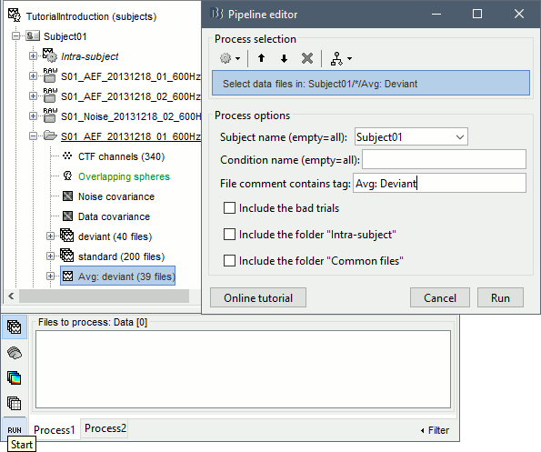
- This process selects all the recordings with a comment including the string "Avg: deviant", from all the folders in Subject01 (except "Intra-subject" and "Common files"). We expect to get two files: the averages of the deviant condition for both runs.
Add process Pre-process > Band-pass filter: Lower cutoff=0Hz, Upper cutoff=30Hz, Mirror.
Add process File > Save snapshot: Recordings time series, Sensors=MEG.
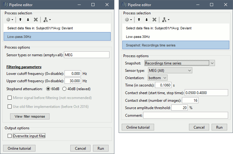
- This will apply a low-pass filter at 30Hz and save a screen capture of the signals in the report.
Do not run the pipeline, select the menu Generate .m script instead. It saves a new .m file and opens it in the Matlab editor. Close the pipeline editor window and look at the script.
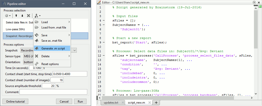
- The script you just generated can be the starting point to your own custom script. The following sections explain line by line how they work and how to edit them.
Line by line: Header
% Script generated by Brainstorm (19-Jul-2016)
All the lines starting with a "%" are comments, they are never executed.
% Input files
sFiles = [];
SubjectNames = {...
    'Subject01'};
These lines define the script inputs:
sFiles: The list of files in input. Currently empty because we did not select anything in input in the Process1 list. If we had selected files, it would contain a cell array of strings with relative file paths.
SubjectNames: List of subject names that are used in the script. Most of the times, the generated script would contain only one entry, but it written as a cell array so that it is easier to extend it to multiple subjects with a loop (described further in this tutorial).
% Start a new report
bst_report('Start', sFiles);
Start a new report of activity: Clears all the previous logs and gets ready to record new messages. The report will collect all the messages that are generated during the execution of the script by the various processes. You can explicitely add screen captures and additional messages to the current report with the function bst_report. This report will remain open until the function bst_report('Start') is called again. To display the current report, use the menu File > Report viewer.
The syntax function_name('SubFunction', arguments) is used a lot in Brainstorm, to call a subfunction available inside a .m file. This line above calls the function Report() in the file brainstorm3/toolbox/process/bst_report.m. This is made possible with the use of the short script "macro_methodcall" you will see at the top of many files. Many of the Brainstorm .m files are actually libraries of functions, rather than simple "scripts" or "functions".
Line by line: Body
% Process: Select data files in: Subject01/*/Avg: deviant
sFiles = bst_process('CallProcess', 'process_select_files_data', sFiles, [], ...
    'subjectname',   SubjectNames{1}, ...
    'condition',     '', ...
    'tag',           'Avg: deviant', ...
    'includebad',    0, ...
    'includeintra',  0, ...
    'includecommon', 0);

% Process: Low-pass:30Hz
sFiles = bst_process('CallProcess', 'process_bandpass', sFiles, [], ...
    'highpass',    0, ...
    'lowpass',     30, ...
    'mirror',      1, ...
    'sensortypes', 'MEG', ...
    'overwrite',   0);

% Process: Snapshot: Recordings time series
sFiles = bst_process('CallProcess', 'process_snapshot', sFiles, [], ...
    'target',         5, ...  % Recordings time series
    'modality',       1, ...  % MEG (All)
    'orient',         4, ...  % bottom
    'time',           0.11, ...
    'contact_time',   [0, 0.1], ...
    'contact_nimage', 12, ...
    'threshold',      20, ...
    'Comment',        'Run');
You will find one block per process you selected in the pipeline editor. They all have the same syntax:
output_files = bst_process('CallProcess', process_name, input_files_A, input_files_B, options_list);
process_name: String indicating the function corresponding to the process to execute. To know from the pipeline editor what is the path to the process function: hover your mouse over the selected process, as illustrated in this tutorial.
input_files_A: List of input files in Process1, or FilesA in Process2. It can be a cell array of files names (full path, or relative path from the protocol folder), or an array of structures describing the files in the database (returned by a previous call to bst_process).
input_files_B: Empty for Process1, or FilesB in Process2. Cell array of strings or array of struct.
options_list: Pairs of (option_name, option_values), one for each option of the process.
output_files: Array of structures describing the files in output of the process. If the process created new files, this variable contains the new files. If the process didn't create new files or was modifying exiting files, most of the time this variable would contain the same files as the input list.
Line by line: Footer
% Save and display report
ReportFile = bst_report('Save', sFiles);
Closes the current report and saves it in the user Brainstorm report folder ($HOME/.brainstorm/reports). These reports are in .mat format and contain all the information necessary to re-run the execution exactly in the same way, but they not easy to read.
The parameter "sFiles" is optional, it indicates what are the files that are considered as the final results of the script. You can remove it without breaking your script: ReportFile = bst_report('Save');
bst_report('Open', ReportFile);Opens the report viewer to display what happened during the execution. This is equivalent to using the menu File > Report viewer. You can comment this line (ie. add a "%" at the beginning of the line) if you don't want to show the report at the end of the execution.
% bst_report('Export', ReportFile, ExportDir);This function exports the report in readable format, as an HTML that includes all the screen captures embedded in it. It is disabled by default. If you want to use this feature: remove the "%" at the beginning of the line, and define the variable ExportDir.
ExportDir must be a string that defines where to save the HTML report. It can be wither the absolute path to a HTML file (eg. 'C:\Users\myuser\Documents\report_example.html') or just a folder (eg. 'C:\Users\myuser\Documents'). If you enter only a path to a folder, a default file name including the protocol name and a date tag is generated (report_ProtocolName_YYMMDD_HHMMSS.html).
Simplify the calls
This script you generated is like any Matlab script: you can edit it, rename the variables, add tests and loops, etc. The first important thing to understand is how to edit the options or change the inputs/outputs of a process. The script generator uses only one variable for all the file lists (sFiles) and the output process is always the input of the following process. This is usually too restrictive to write a full analysis script: we commonly need to have multiple lists of files or to run two different operations on the same file.
Let's consider the first process call, which selects the averages for the Deviant condition in both runs.
sFiles = bst_process('CallProcess', 'process_select_files_data', sFiles, [], ...
    'subjectname',   SubjectNames{1}, ...
    'condition',     '', ...
    'tag',           'Avg: deviant', ...
    'includebad',    0, ...
    'includeintra',  0, ...
    'includecommon', 0);
There is no need to set the parameter sFiles, because there is no input, you can replace it with an empty matrix []. You can therefore remove the line "sFiles = [];". We can also rename the output variable "sAvgData", to be a bit more specific.
sAvgData = bst_process('CallProcess', 'process_select_files_data', [], [], ...You can omit all the options that are not defined, not used, or kept to their default values:
sAvgData = bst_process('CallProcess', 'process_select_files_data', [], [], ...
    'subjectname',   SubjectNames{1}, ...
    'tag',           'Avg: deviant');
Edit low-pass filter call: Change the input to sAvgData and the output to sAvgDataLow, this way you will be able to keep track of the two files if you need to use them independently later in the script.
sAvgDataLow = bst_process('CallProcess', 'process_bandpass', sAvgData, [], ...
    'highpass',    0, ...
    'lowpass',     30, ...
    'sensortypes', 'MEG');
Edit the call to the snapshot process: Change the input to sAvgDataLow, and remove the output parameter (we are not expecting output from it).
bst_process('CallProcess', 'process_snapshot', sAvgDataLow, [], ...
    'target',   5, ...  % Recordings time series
    'modality', 1);     % MEG (All)
Replace the last lines with the following, to export the report instead of opening in the report viewer (edit the file path to point at your own user folder instead).
ReportFile = bst_report('Save');
bst_report('Export', ReportFile, 'C:\Users\franc\Documents\report_test.html');
Evaluate in Matlab
Select the code for the first process in the Matlab editor, right-click > Evaluate selection (or press F9).

If you haven't executed your script yet, you will get the following error in the Matlab command window:
Undefined variable "SubjectNames" or class "SubjectNames".
The variable SubjectNames is not defined yet: Execute the first two lines "SubjectNames = {'Subject01'}", then try again. You should now have a new variable in your Matlab workspace, which points at the two average files. Type "sAvgData(1)" in your command window to display the first element:
>> sAvgData(1)
ans =
          iStudy: 6
           iItem: 1
        FileName: 'Subject01/S01_AEF_20131218_01_600Hz_notch/data_deviant_average_160513_1329.mat'
        FileType: 'data'
         Comment: 'Avg: deviant (39 files)'
       Condition: 'S01_AEF_20131218_01_600Hz_notch'
     SubjectFile: 'Subject01/brainstormsubject.mat'
     SubjectName: 'Subject01'
        DataFile: ''
     ChannelFile: 'Subject01/S01_AEF_20131218_01_600Hz_notch/channel_ctf_acc1.mat'
    ChannelTypes: {'ADC A'  'ADC V'  'DAC'  'ECG'  'EOG'  'FitErr'  'HLU'  'MEG'  'MEG REF' ...}
The field "sAvgData(1).FileName" contains the relative path to the to the Deviant average in the first run. This structure sAvgData contains also a lot of information that can be helpful in your script:
iStudy / iItem: Reference of the file in the database (described later in this tutorial).
FileType: 'raw' (continuous files), 'data' (recordings), 'results' (sources), 'timefreq' (time-frequency, spectrum and connectivity), or 'matrix' (any time series extracted from other files).
Comment: Comment field of the file (what is displayed in the database explorer)
Condition: Name of the condition/folder in which the file is located
SubjectFile: Relative path to the subject file (brainstormsubject.mat)
SubjectName: Name of the subject
DataFile: For types 'results' or 'timefreq', path of the parent file in the database explorer
ChannelFile: Relative path to the channel file
ChannelTypes: Cell array of channel types available for the input file
Naming conventions
To help you navigate in the Brainstorm code, here are some naming conventions:
Structures: Name starting with a "s" followed by a capital letter (eg. sFiles).
Indices: Either loop variables or array indices, name starting with a "i" (eg. iSubject, iStudy, iTime).
Counts: Number of elements in a group, name starting with a "n" (eg. nAvg, nTrials, nSubjects).
File names: Scripts and functions, only lower case, separation with "_" (eg. process_fft, bst_get).
Sub-functions: Inside a .m file, name starting with a capital, CamelCase (eg. CallProcess, Start).
Running the script
The simplified script looks like this:
% Input files
SubjectNames = {'Subject01'};
% Start a new report
bst_report('Start');

% Process: Select data files in: Subject01/*/Avg: deviant
sAvgData = bst_process('CallProcess', 'process_select_files_data', [], [], ...
    'subjectname',   SubjectNames{1}, ...
    'tag',           'Avg: deviant');
% Process: Low-pass:30Hz
sAvgDataLow = bst_process('CallProcess', 'process_bandpass', sAvgData, [], ...
    'highpass',    0, ...
    'lowpass',     30, ...
    'sensortypes', 'MEG');
% Process: Snapshot: Recordings time series
bst_process('CallProcess', 'process_snapshot', sAvgDataLow, [], ...
    'target',   5, ...  % Recordings time series
    'modality', 1);     % MEG (All)

% Save and display report
ReportFile = bst_report('Save');
bst_report('Export', ReportFile, 'C:\Users\franc\Documents\report_test.html');
You have three ways to execute it:
- Select all the lines (Ctrl+A) and evaluate it in Matlab (F9).
- In the Editor toolbar of the Matlab environment, click on the button [Run].
- Save the file, go to this folder with Matlab (or add it to your path) and type the name of the script in the command window (without the ".m" at the end).
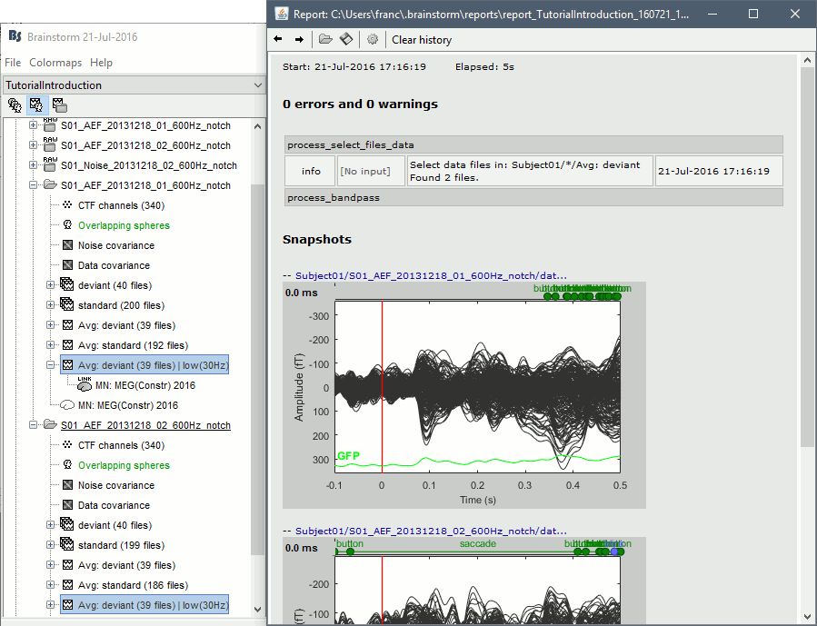
At the end of the execution, nothing happens, because we indicated we wanted to just export the report instead of opening it. To check out the report of execution: use the menu File > Report viewer from the Brainstorm window, or open the report_test.html that was saved somewhere on your computer.
On this page, you can get review everything that happened in the script: when it was executed, how long it took, what are the processes that were executed, some produced messages (two files were selected with the first process), and at the end you have the screen captures taken by process_snapshot.
Running the script again
If you execute the script again, it will not behave as expected anymore. The selection process we used assumes that there is only one file per folder with a comment that includes "Avg: deviant". This is not the case anymore after the execution, because the low-pass filtered files also contain the same tags. The execution of the first process of the script now returns 4 files.
>> sAvgData = bst_process('CallProcess', 'process_select_files_data', [], [], ...
    'subjectname',   SubjectNames{1}, ...
    'tag',           'Avg: deviant')

sAvgData =
1x4 struct array with fields:
    iStudy
    iItem
    ...
In order to exclude the low-pass filtered files from this selection, you can add another process that will refine the selection. Use the script generator again to create a template call for another process, then copy-paste it in your script.
- In Process1: Select any recordings file (we will not run anything, just generate a script).
Select process File > Select files: By tag: Search="low", Search the comment, Ignore the files.
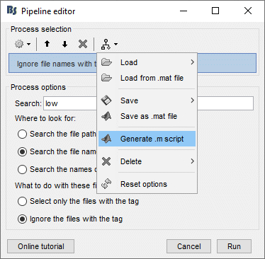
Select the menu Generate .m script (make sure you do not overwrite the script you are currently working on), then close the pipeline editor.
- Copy-paste and edit the call to process_select_tag to your main script.
Now the file selection part of your script should look like this, and should return only two files:
% Process: Select data files in: Subject01/*/Avg: Deviant
sAvgData = bst_process('CallProcess', 'process_select_files_data', [], [], ...
    'subjectname',   SubjectNames{1}, ...
    'tag',           'Avg: deviant');
% Process: Ignore file comments with tag: low
sAvgData = bst_process('CallProcess', 'process_select_tag', sAvgData, [], ...
    'tag',    'low', ...
    'search', 2, ...  % Search the file comments
    'select', 2);  % Ignore the files with the tag
With this last modification, your script is more robust. It can be executed multiple times without completely changing its behavior. When you are fetching files from the database using comment tags or file names, always pay attention to this aspect: the database grows and the further you go, the more specific your requests have to be.
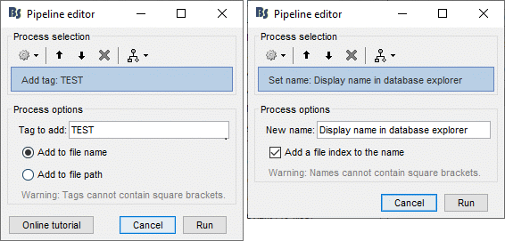
A good practice can be to tag explicitely the output files your script generates if you need to fetch them later. You can use the process File > Add tag and File > Set comment.
Starting Brainstorm
Brainstorm must be running in the background for these scripts to run properly. The interface doesn't have to be visible on the screen, but the database engine must be running for processing requests. At the beginning of your script, you can explicitely start or restart Brainstorm.
brainstorm: Start Brainstorm with the regular GUI.
brainstorm nogui: Start in silent mode, without the GUI, without progress bar, without user interactions.
If you want to start Brainstorm only if Brainstorm is not already running, you can use the following code:
if ~brainstorm('status')
    brainstorm nogui
end
To select a specific protocol at the beginning of your script:
ProtocolName = 'TutorialIntroduction';
% Get the protocol index
iProtocol = bst_get('Protocol', ProtocolName);
if isempty(iProtocol)
    error(['Unknown protocol: ' ProtocolName]);
end
% Select the current procotol
gui_brainstorm('SetCurrentProtocol', iProtocol);
To delete the protocol and start over:
% Delete existing protocol
gui_brainstorm('DeleteProtocol', ProtocolName);
% Create new protocol
gui_brainstorm('CreateProtocol', ProtocolName, 0, 0);
Database requests
The functions bst_get and bst_set allow you to query the database, access the configuration of the software and some display parameters. The complete reference documentation of these functions is included directly in their code (brainstorm3/toolbox/core/bst_get.m and bst_set.m).
Let's start with a few simple examples:
>> ProtocolInfo = bst_get('ProtocolInfo')  % Returns the configuration of the current protocol
ProtocolInfo =
              Comment: 'TutorialIntroduction'
              STUDIES: 'C:\Work\Protocols\TutorialIntroduction\data'
             SUBJECTS: 'C:\Work\Protocols\TutorialIntroduction\anat'
               iStudy: 6
       UseDefaultAnat: 0
    UseDefaultChannel: 0

>> isGUI = bst_get('isGUI')   % Is the Brainstorm interface currently displayed (0=no, 1=yes)

>> bst_set('FlipYAxis', 1)                 % The new figures will have the Y axis flipped
>> bst_set('TSDisplayMode', 'butterfly')   % The new figures will use a "butterfly" view
>> bst_set('FieldTripDir', FieldTripDir)   % Set the path where the FieldTrip toolbox is installed
To reference the files in the database, each protocol is subdivided in Subjects (the "anat" folder and containing the MRI, surfaces and atlases) and Studies (the "data" folder, including the recordings, channel files and all the analyses). Each Study corresponds to a sub-folder (eg. protocol/data/subject01/run01/), and is attached to only one subject.
Subjects and Studies are referenced in the protocol with a unique index most of the time kept in variables named iSubject and iStudy. The files available in them are also referenced with indices, with variables such as iAnatomy, iSurface, iData, iHeadModel, iResults, iTimefreq. You can see the indices in the database explorer by hovering your mouse over the nodes of the tree:

Example: Getting the study structure from the variable sAvgData, defined in the script:
>> sAvgData(1)
ans =
          iStudy: 6
           iItem: 1
           ...

>> sStudy = bst_get('Study', sAvgData(1).iStudy)     % Get a study structure with its index
sStudy =
                 Name: 'S01_AEF_20131218_01_600Hz_notch'
             FileName: 'Subject01/S01_AEF_20131218_01_600Hz_notch/brainstormstudy.mat'
          DateOfStudy: '13-May-2016'
    BrainStormSubject: 'Subject01/brainstormsubject.mat'   % Corresponding subject filename
            Condition: {'S01_AEF_20131218_01_600Hz_notch'} % Name of the condition (=folder)
              Channel: [1x1 struct]                        % Channel file for the folder
             iChannel: []                                  % Not used anymore
                 Data: [1x242 struct]                      % List of "data" files in the folder
            HeadModel: [1x1 struct]                        % List of head models in the folder
           iHeadModel: 1                                   % Default head model (file in green)
               Result: [1x244 struct]                      % List of source files and source links
                 Stat: [1x0 struct]                        % List of statistical results
                Image: [0x0 struct]                        % List of images
             NoiseCov: [1x2 struct]                        % Noise(1) and data(2) covariance files
              Dipoles: [0x0 struct]                        % List of dipole files in the folder
             Timefreq: [1x247 struct]                      % List of time-frequency files
               Matrix: [0x0 struct]                        % List of "matrix" files in the folder
                       % If 1, the trial is marked as bad in the explorer
Example: Getting the data structure.
>> sData = sStudy.Data(sAvgData(1).iItem)    % Get the structure representing the file from sStudy
sData =
    FileName: 'Subject01/S01_AEF_20131218_01_600Hz_notch/data_deviant_average_160513_1329.mat'
     Comment: 'Avg: deviant (39 files)'      % File comment, displayed in the database explorer
    DataType: 'recordings'                   % Type of data in the file (mostly "recordings")
    BadTrial: 0
Example: Getting the subject structure.
>> sSubject = bst_get('Subject', sStudy.BrainStormSubject)   % Get subject structure from filename
sSubject =
                 Name: 'Subject01'         % Subject name, same as folder name
             Comments: ''                  % Not used much
             FileName: 'Subject01/brainstormsubject.mat'
    DateOfAcquisition: ''                  % Not used anymore
              Anatomy: [1x1 struct]        % List of MRI volumes in the subject folder
              Surface: [1x9 struct]        % List of surfaces in the subject folder
             iAnatomy: 1                   % Default MRI volume (in green, index of array Anatomy)
               iScalp: 9                   % Default head surface (index of array Surface)
              iCortex: 4                   % Default cortex surface (index of array Surface)
          iInnerSkull: []                  % Default inner skull surface (index of array Surface)
          iOuterSkull: []                  % Default outer skull surface (index of array Surface)
               iOther: []                  % Not used anymore
       UseDefaultAnat: 0                   % If 1: Subject uses the default anatomy
    UseDefaultChannel: 0                   % 0=one channel/folder, 1=one/subject, 2=one global
Example: Getting the study structure and data index from a file name.
>> DataFile = sAvgData(1).FileName
DataFile =
Subject01/S01_AEF_20131218_01_600Hz_notch/data_deviant_average_160513_1329.mat

>> [sStudy, iStudy, iData] = bst_get('DataFile', DataFile)
sStudy =
                 Name: 'S01_AEF_20131218_01_600Hz_notch'
             FileName: 'Subject01/S01_AEF_20131218_01_600Hz_notch/brainstormstudy.mat'
          DateOfStudy: '13-May-2016'
    BrainStormSubject: 'Subject01/brainstormsubject.mat'
            Condition: {'S01_AEF_20131218_01_600Hz_notch'}
              Channel: [1x1 struct]
             iChannel: []
                 Data: [1x242 struct]
            HeadModel: [1x1 struct]
           iHeadModel: 1
               Result: [1x244 struct]
                 Stat: [1x0 struct]
                Image: [0x0 struct]
             NoiseCov: [1x2 struct]
              Dipoles: [0x0 struct]
             Timefreq: [1x247 struct]
               Matrix: [0x0 struct]
iStudy =
     6
iData =
     1
Many other options are available for searching files in the database with bst_get. We cannot list them all in this page, but you can refer to the code of bst_get.m for more information.
To change parameters or database structures: bst_set.m.
File manipulation [TODO]
- Modify a structure manually: Export to Matlab/Import from Matlab
- File manipulation: file_short, file_fullpath, in_bst_*...
- Documentation of all file structures: point at the appropriate tutorials
- Select files from the database (with bst_get and processes)
- Reading / writing / exporting functions
Reloading the database to update modifications in the file system:
Additional quality control
Create figures and snapshot them
Generate warnings and errors
Loop over subject and runs [TODO]
Creating loops is not supported yet by the script generator, but relatively easy to do from a script without having to know too much about Matlab programming.
1) Fill the cell array SubjectNames with all your subjects names, with the same dimensions as the list of input raw files (sFiles)
- 2) Add a "for" loop that includes all the bst_process() calls (leave the bst_report() calls and input definition outside)
3) Inside the loop, replace SubjectNames with SubjectNames{i} and sFiles with sFiles(i)
How to process an entire study
This section proposes a standard workflow for processing a full group study with Brainstorm. It contains the same steps of analysis as the introduction tutorials, but separating what can be done automatically from what should be done manually. This workflow can be adapted to most ERP studies (stimulus-based).
Prototype: Start by processing one or two subjects completely interactively (exactly like in the introduction tutorials). Use the few pilot subjects that you have for your study to prototype the analysis pipeline and check manually all the intermediate stages. Take notes of what you're doing along the way, so that you can later write a script that reproduces the same operations.
Anatomical fiducials: Set NAS/LPA/RPA and compute the MNI transformation for each subject.
Segmentation: Run FreeSurfer/BrainSuite to get surfaces and atlases for all the subjects.
File > Batch MRI fiducials: This menu prompts for the selection of the fiducials for all the subjects and saves a file fiducials.m in each segmentation folder. You will not have to redo this even if you have to start over your analysis from the beginning.
Script: Write a loop that calls the process "Import anatomy folder" for all the subjects.
Alternatives: Create and import the subjects one by one and set the fiducials at the import time. Or use the default anatomy for all the subjects (or use warped templates).
Script #1: Pre-processing: Loop on the subjects and the acquisition runs.
Create link to raw files: Link the subject and noise recordings to the database.
Event markers: Read and group triggers from digital and analog channel, fix stimulation delays
Evaluation: Power spectrum density of the recordings to evaluate their quality.
Pre-processing: Notch filter, sinusoid removal, band-pass filter.
Evaluation: Power spectrum density of the recordings to make sure the filters worked well.
Cleanup: Delete the links to the original files (the filtered ones are copied in the database).
Detect artifacts: Detect heartbeats, Detect eye blinks, Remove simultaneous.
Compute SSP: Heartbeats, Blinks (this selects the first component of each decomposition)
Compute ICA: If you have some artifacts you'd like to remove with ICA (no default selection).
Screenshots: Check the MRI/sensors registration, PSD before and after corrections, SSP.
Export the report: One report per subject, or one report for all the subjects, saved in HTML.
Manual inspection #1:
Check the reports: Information messages (number of events, errors and warnings) and screen captures (registration problems, obvious noisy channels, incorrect SSP topographies).
Mark bad channels: Open the recordings, select the channels and mark them as bad. Or use the process "Set bad channels" to mark the same bad channels in multiple files.
Fix the SSP/ICA: For the suspicious runs: Open the file, adjust the list of blink and cardiac events, remove and recompute the SSP decompositions, manually select the components.
Detect other artifacts: Run the process on all the runs of all the subjects at once (select all the files in Process1 and run the process, or generate the equivalent script).
Mark bad segments: Review the artifacts detected in 1-7Hz and 40-240Hz, keep only the ones you really want to remove, then mark the event categories as bad. Review quickly the rest of the file and check that there are no other important artifacts.
Additional SSP: If you find one type of artifact that repeats (typically saccades and SQUID jumps), you can create additional SSP projectors, either with the process "SSP: Generic" or directly from a topography figure (right-click on the figure > Snapshot> Use as SSP projector).
Script #2: Subject-level analysis: Epoching, averaging, sources, time-frequency.
Importing: Process "Import MEG/EEG: Events" and "Pre-process > Remove DC offset".
Averaging: Average trials by run, average runs by subject (registration problem in MEG).
Noise covariance: Compute from empty room or resting recordings, copy to other folders.
Head model: Compute for each run, or compute once and copy if the runs are co-registered.
Sources: Compute for each run, average across runs and subjects in source space for MEG.
Time-frequency: Computation with Hilbert transform or Morlet wavelets, then normalize.
Screenshots: Check the quality of all the averages (time series, topographies, sources).
Export the report: One report per subject, or one report for all the subjects, saved in HTML.
Manual inspection #2:
Check the reports: Check the number of epochs imported and averaged in each condition, check the screen capture of the averages (all the primary responses should be clearly visible).
Regions of interest: If not using predefined regions from an atlas, define the scouts on the anatomy of each subject (or on the template and then project them to the subjects).
Script #3: Group analysis, ROI-based analysis, etc.
Averaging: Group averages for the sensor data, the sources and the time-frequency maps.
Statistics: Contrast between conditions or groups of subjects.
Regions of interest: Any operation that involve scouts.
Final script
The following script from the Brainstorm distribution reproduces the introduction tutorials ("Get started"): brainstorm3/toolbox/script/tutorial_introduction.m
For an example of a script illustrating how to create loops, look at the tutorial MEG visual: single subject. brainstorm3/toolbox/script/tutorial_visual_single.m
Report viewer
Click on Run to start the script.
As this process is taking screen captures, do not use your computer for something else at the same time: if another window covers the Brainstorm figures, it will not capture the right images.
At the end, the report viewer is opened to show the status of all the processes, the information messages, the list of input and output files, and the screen captures. The report is saved in your home folder ($home/.brainstorm/reports). If you close this window, you can get it back with the menu File > Report viewer.

