|
Size: 31392
Comment:
|
Size: 35448
Comment:
|
| Deletions are marked like this. | Additions are marked like this. |
| Line 35: | Line 35: |
| The minimum norm estimates gives a measure of the current density flowing at the surface of the cortex. To visualize these results and compare them between subjects, we can normalize the MNE values to get a standardized level of activation with respect to the noise or baseline level (dSPM, sLORETA, MNp). | The minimum norm estimates are a measure of the current density flowing at the surface of the cortex. To visualize these results and compare them between subjects, we can normalize the MNE values to get a standardized level of activation with respect to the noise or baseline level (dSPM, sLORETA, MNp). |
| Line 39: | Line 39: |
| * '''sLORETA''': Noise-normalized estimate using the sLORETA approach (standardized LOw Resolution brain Electromagnetic TomogrAphy [Pasqual-Marqui, 2002]). sLORETA solutions have in general a smaller location bias than either the expected current (MNE) or the dSPM. <<BR>>Units: Unitless ratio [ '''???''' ] | * '''sLORETA''': Noise-normalized estimate using the sLORETA approach (standardized LOw Resolution brain Electromagnetic TomogrAphy [Pasqual-Marqui, 2002]). sLORETA solutions have in general a smaller location bias than either the expected current (MNE) or the dSPM. <<BR>>Units: [ '''???''' ] |
| Line 103: | Line 103: |
| * Right-click on the '''head model''' or on the '''folder '''for Run#01 > Compute sources [2015].<<BR>>Select the options: '''Minimum norm''' imaging, '''Current density''' map, '''Unconstrained'''<<BR>><<BR>> {{attachment:minnorm_shared_popup.gif||height="305",width="496"}} | * Right-click on the '''head model''' or the '''folder '''for Run#01 > '''Compute sources [2015]'''.<<BR>>Select the options: '''Minimum norm''' imaging, '''Current density''' map, '''Unconstrained'''<<BR>><<BR>> {{attachment:minnorm_shared_popup.gif||height="305",width="496"}} |
| Line 110: | Line 110: |
| * We have to be careful with the visual comparisons of constrained and unconstrained source maps displayed on the cortex surface, because they are very different types of data. In unconstrained source maps, we have '''three dipoles with orthogonal orientations at each cortex location''', therefore we cannot represent at once all the information. To represent them, Brainstorm first extracts the '''norm of the vectorial sum of the three orientations at each vertex'''. <<BR>><<BR>> {{attachment:minnorm_unconstr_sketch.gif}} | * We have to be careful with the visual comparisons of constrained and unconstrained source maps displayed on the cortex surface, because they are very different types of data. In unconstrained source maps, we have '''three dipoles with orthogonal orientations at each cortex location''', therefore we cannot represent at once all the information. To display them as an activity map, Brainstorm computes the '''norm of the vectorial sum of the three orientations at each vertex'''. <<BR>><<BR>> {{attachment:minnorm_unconstr_sketch.gif||height="158",width="476"}} |
| Line 125: | Line 125: |
| * In Run#01, right-click on the average recordings for the '''deviant''' stim > '''Compute sources [2015]'''.<<BR>>Select sucessively the three normalization options: dSPM, sLORETA, MNp (constrained/normal). * (''TODO: This is currently under development, sLORETA solution is not available yet'') SCREEN CAPTURES |
* In Run#01, right-click on the average recordings for the '''deviant''' stim > '''Compute sources [2015]'''.<<BR>>Select sucessively the three normalization options: dSPM, sLORETA, MNp ('''unconstrained''').<<BR>><<BR>> {{attachment:minnorm_normfiles.gif}} * Double-click on all of them to compare them: <<BR>><<BR>> {{attachment:minnorm_normalized.gif||height="264",width="374"}} * '''Current density maps''': Tends to highlight the top of the gyri and the superficial sources. * '''dSPM''': Tends to correct that behavior and may give higher values in deeper areas. * '''sLORETA''': produces a very smooth solution where all the potentially activated area of the brain (given to the low spatial resolution of the source localization with MEG/EEG) is shown as connected, regardless of the depth of the sources. * '''MNp''': ??? |
| Line 132: | Line 138: |
| SCREEN CAPTURE | * The '''Z-transformation''' converts the current density values to a score of deviation from a baseline. For each source separately we define a baseline, compute the average and standard deviation for this segment. Then for every time point we subtract the baseline average and divide by the baseline standard deviation. It tells how much a value deviates from the average at rest (in number of times the standard deviation). * Drag and drop the unconstrained current density maps (the only link) to the Process1 list. * Run process "'''Standardize > Z-score normalization'''", baseline = '''[-100,-2]ms.''' <<BR>>Select the option "'''Use the norm of the three orientations'''", if not it would compute the Z-score normalization separately for each direction and then take the norm of the three Z-scored orientation for display, which doesn't make a lot of sense.<<BR>> The option "dynamic" offers an optimization in the storage of the Z-scored file that can save a lot of disk space in some cases, but that is compatible with the "norm" option for unconstrained sources.<<BR>><<BR>> {{attachment:zscore_process.gif||height="328",width="524"}} * The option "absolute values / norm of the three orientations" caused the call to the intermediate process "'''Sources > Unconstrained to flat map''': norm". This is why the comment of the output file includes the tag "'''norm'''". <<BR>>Note that this process brought down the number of signals in the file from 45,000 (the number of dipoles) to 15,000 (the number of grid points). There is now only one normalized value for each vertex of the cortex surface. {{attachment:zscore_cortex.gif||height="143",width="408"}} * If the baseline and the active state are not in the same file, you can use the '''Process2 tab''': place the baseline in the left list (Files A) and the file to normalize in the right list (Files B). ==== Delete your experiments ==== * Select all the normalized source maps (everything but the link) and '''delete''' them. <<BR>><<BR>> {{attachment:delete_norm.gif||height="134",width="447"}} |
| Line 137: | Line 151: |
| * Averaging across MEG runs. | * Averaging single trials across MEG runs. |
| Line 140: | Line 154: |
| * Calculating sources for average responses * Exploring visually the ERP/ERF at the source level, * Normalizing the subjects condition averages before a group analysis. * '''sLORETA, Kernel only, Unconstrained''' * Open solutions #3 (wMNE), #4 (dSPM) and #5 (sLORETA), all unconstrained. * Notice that the units are different: wMNE values are in pAm, dSPM and sLORETA are in arbitrary units (never try to compare these values to anything but the exact same type of inverse solution) * Observe around 46ms the respective behavior of these three solutions: * 3) wMNE tends to highlight the top of the gyri and the superficial sources, * 4) dSPM tends to correct that behavior and may give higher values in deeper areas, * 5) sLORETA produces a very smooth solution where all the potentially activated area of the brain (given to the low spatial resolution of the source localization with MEG/EEG) is shown as connected, regardless of the depth of the sources.<<BR>> Now delete all these files when you're done, and keep only the initial solution: wMNE, Constrained. |
* Estimating the sources for an average response. * Exploring visually the ERP/ERF at the source level. * Normalizing the subjects averages before a group analysis. |
| Line 154: | Line 159: |
| * Now we have the source maps available for all the trials, we average them in source space. * Select the folders for '''Run01 '''and '''Run02 '''and the ['''Process sources'''] button on the left. * Run process "'''Average > Average files'''": Select "'''By trial group (subject average)'''" . {{http://neuroimage.usc.edu/brainstorm/Tutorials/Auditory?action=AttachFile&do=get&target=process_average_results.gif|process_average_results.gif|height="376",width="425",class="attachment"}} * Double-click on the source averages to display them (standard=top, deviant=bottom). . {{http://neuroimage.usc.edu/brainstorm/Tutorials/Auditory?action=AttachFile&do=get&target=average_source.gif|average_source.gif|height="321",width="780",class="attachment"}} |
* First compute the same source model for the the second acquisition run.<<BR>>In Run#02, right-click on the '''head model''' or the '''folder '''> '''Compute sources [2015]'''.<<BR>>Select the options: '''Minimum norm''' imaging, '''Current density''' map, '''Unconstrained'''<<BR>><<BR>> {{attachment:minnorm_run02.gif||height="227",width="240"}} * Now we have the source maps available for all the trials, we can '''average them in source space''' across runs. This allows us to average MEG recordings that were recorded with different head positions (in this case Run#01 and Run#02 have different channel files so they could potentially have different head positions preventing the direct averaging at the sensor level). * Thanks to the linearity of the minimum norm model, the two following approaches are equivalent: * Averaging the sources of all the individual trials across runs, * Averaging the sources for the sensor averages that we already computed for each run. For non-standardized current density maps: MN(Average(trials)) = Average(MN(trials)) * The second solution is a lot faster because it needs to read 4 files (one file per run and per condition) instead of 480 (total number of trials in the two runs). * Drag and drop to the Process1 tab the average recordings for '''Run01 '''and '''Run02''', then press the ['''Process sources'''] button on the left. * Run process "'''Average > Average files'''": Select "'''By trial group (subject average)'''". <<BR>>The options "trial group" average together the files that have similar comments.<<BR>><<BR>> {{attachment:average_process.gif||height="446",width="449"}} * The two averages that are produced (one for each condition) are saved in the folder '''Intra-subject'''. This is where all the files that were computed using information from multiple folders within the same subject are going to be saved. If you prefer to have them in different folders, you can always move create new folders and move them there. <<BR>><<BR>> {{attachment:average_files.gif}} * Clear the Process1 list, then drag and drop the new averages in it.<<BR>>Run process "'''Standardize > Z-score normalization'''", baseline = '''[-100,-2]ms.''' <<BR>>Select the option "'''Use the norm of the three orientations'''"<<BR>><<BR>> {{attachment:average_zscore.gif||height="301",width="487"}} * Double-click on the source averages to display them (standard=top, deviant=bottom). <<BR>>You can the average recordings of one or the other run for adding a time reference. <<BR>>Use the pre-defined view "Left, Right" for looking at the two sides at once (shortcut: "7").<<BR>><<BR>> {{attachment:average_display_zscore.gif|average_display.gif|height="269",width="547"}} |
| Line 161: | Line 171: |
| * Warning: This approach is valid only for the current density maps. In general, it is '''not advised to average normalized source maps '''because the average of the normalized maps is not the same as the normalization of the average. '''First average, then normalize'''. This issue is described in an advanced section below. | |
| Line 165: | Line 176: |
| * '''Standard:''' (Right-click on the 3D figures > Snapshot > Time contact sheet) . Explain qhat to do to make nice contact sheets this way * '''Deviant:''' . {{http://neuroimage.usc.edu/brainstorm/Tutorials/Auditory?action=AttachFile&do=get&target=average_source_deviant_left.gif|average_source_deviant_left.gif|height="263",width="486",class="attachment"}} * Contact sheets: in time or in space, for each orientation. You can try all the menus. Example: Right-click on the figure > Snapshot > Volume contact sheet: axial: <<BR>><<BR>> {{attachment:popupSnapshot.gif}} {{attachment:contactAxial.gif||height="288px",width="322px"}} * '''Movies''': Right-click on any figure > Snapshot > '''Movie (time): All figures''' (click to download video) [[http://neuroimage.usc.edu/wikidocs/average_sources.avi|{{http://neuroimage.usc.edu/brainstorm/Tutorials/Auditory?action=AttachFile&do=get&target=average_source_video.gif|http://neuroimage.usc.edu/brainstorm/wikidocs/average_sources.avi|height="258",width="484",class="attachment"}}]] |
A good way to represent what is happening in time is to generate contact sheets or videos. Right-click on any figure and go to the menu Snapshot to check out all the possible options. For a nicer result, take some time to adjust the size of the figure, the amplitude threshold and the colormap options (hiding the colorbar can be a good option for contact sheets). A time stamp is added to the captured figure. The size of the text font is fixed, so if you want it to be reable in the contact sheet, you should make you figure very small before starting the capture. * '''Contact sheet:''' Right-click on any figure > Snapshot > '''Time contact sheet: Figure'''<<BR>><<BR>> {{attachment:contact_options.gif}} {{attachment:contact_image.gif}} * '''Movies''': Right-click on any figure > Snapshot > '''Movie (time): All figures''' (click to download video) {{attachment:video_options.gif||height="263",width="126"}} [[http://neuroimage.usc.edu/wikidocs/average_sources_unconstr.avi|{{attachment:video_vlc.gif|http://neuroimage.usc.edu/wikidocs/average_sources_unconstr.avi|height="262",width="409"}}]] |
Tutorial 22: Source estimation
[UNDER CONSTRUCTION]
Authors: Francois Tadel, Elizabeth Bock, Rey R Ramirez, John C Mosher, Richard Leahy, Sylvain Baillet
You have in your database a forward model matrix that explains how the cortical sources determine the values on the sensors. This is useful for simulations, but what we need is to build the inverse information: how to estimate the sources when we have the recordings. This tutorials introduces the tools available in Brainstorm for solving this inverse problem.
Contents
- Ill-posed problem
- Source estimation options [TODO]
- Sources for a single data file (constrained)
- Display: Cortex surface
- Display: MRI Viewer
- Display: MRI 3D
- Sign of constrained minimum norm values
- Computing sources for multiple data files
- Source map normalization
- Average in source space
- Display: Contact sheets and movies
- Advanced options
- Equations
- Rey on sLORETA
- Issues with dSPM average
- On the hard drive
- References
- Additional discussions on the forum
Ill-posed problem
Our goal is to estimate the activity of the 45,000 dipoles described by our forward model. However we only have a few hundreds of variables (the number of sensors). This inverse problem is ill-posed, there is an infinity of combinations of source activity that can generate exactly the same sensor topography. Inverting the forward problem directly is impossible, unless we add some strong priors in our model.
Wikipedia says: "Inverse problems are some of the most important and well-studied mathematical problems in science and mathematics because they tell us about parameters that we cannot directly observe. They have wide application in optics, radar, acoustics, communication theory, signal processing, medical imaging, computer vision, geophysics, oceanography, astronomy, remote sensing, natural language processing, machine learning, nondestructive testing, and many other fields."
Many solutions have been proposed in the literature, based on different assumptions on the way the brain works and depending on the amount of information we already have on the effects we are studying. Among the hundreds of methods available, two classes of inverse models have been widely used in MEG/EEG source imaging in the past years: minimum-norm solutions and beamformers.
Both approaches have the advantage of being linear: the activity of the sources is a linear recombination of the MEG/EEG recordings. It is possible to solve the inverse problem independently of the recordings, making the data manipulation a lot easier and faster.
Both are available in Brainstorm, so you can use the one the most adapted to your recordings or to your own personal expertise. Only the minimum norm estimates will be described in this tutorial, but the other solutions work exactly in the same way.
Source estimation options [TODO]
Before we start estimating the sources for the recordings available in our database, let's start with an overview of the options available. The screen capture below represents the basic options for the minimum norm estimates. The options for the other methods will be described in advanced tutorials.
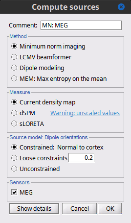
Method
Minimum norm: Priors, justification, application case?
Require an estimation of the noise at the level of the sensors (noise covariance matrix).Dipole modeling: ?
LCMV beamformer: ?
Require both a noise covariance matrix and a data covariance matrix (representation of the effect we are trying to localize in the brain, covariance of the latencies of interest).Recommended option: Provided that we know at what latencies to look at, we can compute a correct data covariance matrix and may obtain a better spatial accuracy with a beamformer. However, in many cases we don't exactly know what we are looking at, the risks of misinterpretation of badly designed beamforming results are high. Brainstorm tends to favor minimum norm solutions, which have the advantage of needing less manual tuning for getting acceptable results.
Measure
The minimum norm estimates are a measure of the current density flowing at the surface of the cortex. To visualize these results and compare them between subjects, we can normalize the MNE values to get a standardized level of activation with respect to the noise or baseline level (dSPM, sLORETA, MNp).
Current density map: Whitened and depth-weigthed linear L2-minimum norm estimates algorithm inspired from Matti Hamalainen's MNE software. For a full description of this method, please refer to the MNE manual, section 6, "The current estimates".
Units: picoamper per meter (pA.m).dSPM: Noise-normalized estimate (dynamical Statistical Parametric Mapping [Dale, 2000]). Its computation is based on the MNE solution.
Units: Unitless ratio [ ??? ]sLORETA: Noise-normalized estimate using the sLORETA approach (standardized LOw Resolution brain Electromagnetic TomogrAphy [Pasqual-Marqui, 2002]). sLORETA solutions have in general a smaller location bias than either the expected current (MNE) or the dSPM.
Units: [ ??? ]MNp: ?
Units: Unitless ratio [ ??? ]Recommended option: Discussed in the section "Source map normalization"
Source orientation
Constrained: Normal to cortex: Only one dipole at each vertex of the cortex surface, oriented normally to the surface. This is based on the anatomical observation that in the cortex, the neurons are mainly organized in macro-columns that are perpendicular to the cortex surface.
Size of the inverse operator: [nVertices x nChannel].Constrained: Optimal orientation: Only one dipole at each vertex of the cortex surface, oriented normally to the surface. This is based on the anatomical observation that in the cortex, the neurons are mainly organized in macro-columns that are perpendicular to the cortex surface.
Size of the inverse operator: [nVertices x nChannel].Unconstrained: At each vertex of the cortex surface, we define a base of three dipoles with orthogonal directions, then we estimate the sources for the three orientations independently.
Size of the inverse operator: [3*nVertices x nChannel].Loose: A version of the "unconstrained" option with a weak orientation constraint that emphasizes the importance of the sources with orientations that are close to the normal to the cortex. The value associated with this option set how "loose" should be the orientation constrain (recommended values in MNE are between 0.1 and 0.6, --loose option).
Size of the inverse operator: [3*nVertices x nChannel].Recommended option: ?
The constrained options use one dipole per orientation instead of three, therefore the source maps are smaller, faster to compute and display, and much more intuitive to process because we don't have to think about recombining the three values in one. However the normal orientation constraint is most of the time too strong and not realistic.
Unconstrained sources look smoother and nicer but are not necessarily more accurate.
Sources for a single data file (constrained)
In Run#01, right-click on the average response for the deviant stim > Compute sources [2015].
Select the options: Minimum norm imaging, Current density map, Constrained: Normal to cortex.
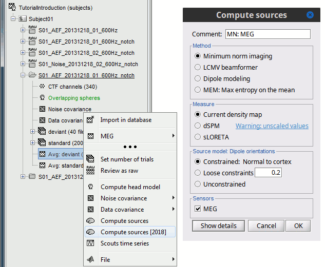
- The other menu "Compute sources" brings the interface that was used previously in Brainstorm. We are going to keep maintaining the two implementations in parallel for a while for compatibility and cross-validation purposes.
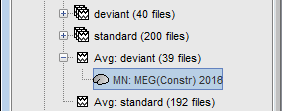
The result of the computation is displayed as a dependent of the deviant average because it is related only to this file. In the file comment, "MN" stands minimum norm and "Constr" stands for "Constrained: normal orientation".
Display: Cortex surface
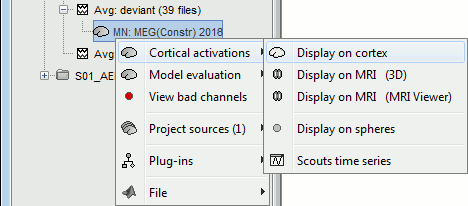
Right-click on the sources for the deviant average > Cortical activations > Display on cortex.
Double-click on the recordings for the deviant average to have time reference.
In the filter tab, add a low-pass filter at 100Hz.
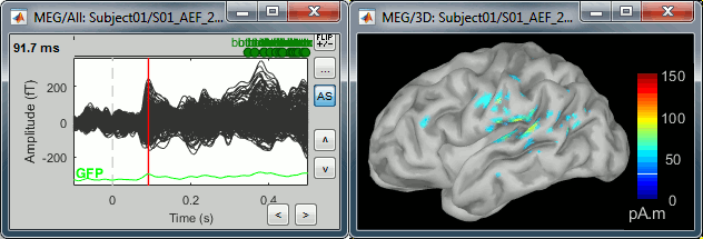
- Change the current time (click on the time series figure or use the keyboard arrows) and note it updates the source maps in the 3D figure. You can also use all the menus and shortcuts introduced in the anatomy tutorial (like setting the view with the keys from 0 to 6).
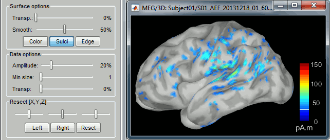
- You can edit many display properties from the Surface tab:
Amplitude: Only the sources that have a value superior than a given percentage of the colorbar maximum are displayed.
Min. size: Hide all the small activated regions, ie. the connected color patches that contain a number of vertices smaller than this "min size" value.
Transparency: Change the transparency of the sources on the cortex.
Take a few minutes to understand what the amplitude threshold represents.
The colorbar maximum depends on the way you configured your Sources colormap. If the option "Maximum: Global" is selected, the maximum should be around 30 pA.m. This value is a rough estimate of the maximum amplitude, sometimes you may have to redefine it manually.
On the screen capture below, the threshold value is set to 90%. It means that only the sources that have a value over 0.90*30 = 27 pA.m are visible.
The threshold level is indicated in the colorbar with a horizontal white line.
At the first response peak (91ms), the sources with high amplitudes are located around the primary somatosensory cortex, which is what we are expecting for an auditory stimulation.
Display: MRI Viewer
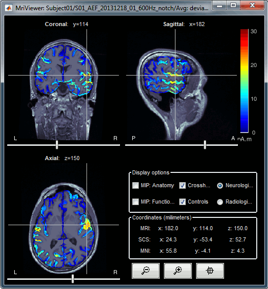
Right-click on the source file > Cortical activations > Display on MRI (MRI Viewer).
The MRI viewer was introduced in tutorials #2 and #3.
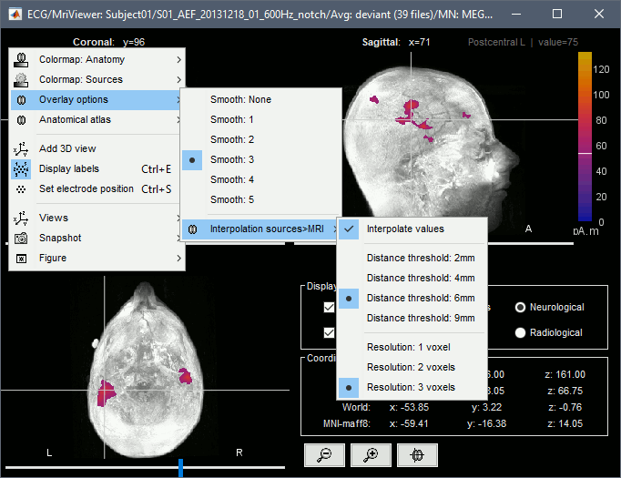
Additionally you can change the current time and amplitude threshold from the Brainstorm window.This figure shows the sources computed on the surface surface and re-interpolated in the MRI volume. If you set the amplitude threshold to 0%, you would see the thin layer of cortex in which the dipoles where estimated.
- You can configure this figure with the following options:
MIP Anatomy: Checkbox in the MRI Viewer figure. For each slice, display the maximum value over all the slices instead of the original value in the structural MRI ("glass brain" view).
MIP Functional: Same thing but with the layer of functional values.
Smooth level: The sources values can be smoothed after being re-interpolated in the volume. Right-click on the figure to define the size of the smoothing kernel.
Amplitude threshold: In the Surface tab of the Brainstorm window.
Current time: At the top-right of the Brainstorm window (or use the time series figure).
Display: MRI 3D
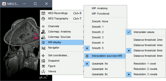
Right-click on the source file > Cortical activations > Display on MRI (3D).
This view was also introduced in the tutorials about MRI and surface visualization.
Right-click and move your mouse to move the slices.
Sign of constrained minimum norm values
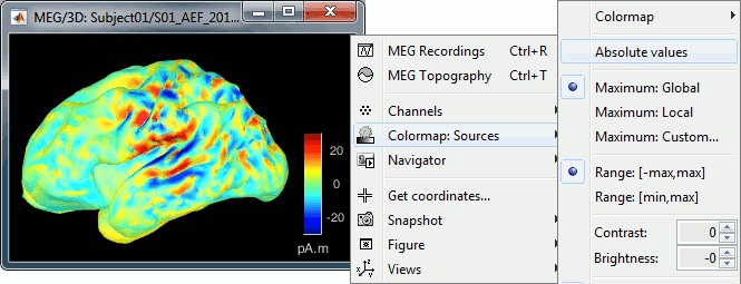
You should pay attention to a property of the current amplitudes that are given by the minimum norm method: they can be positive of negative, and they oscillate around zero. If you display the sources of the surface again, then configure the colormap to show relative values (uncheck the "Absolute values" option), you would see those typical stripes of positive and negative values around the sulci. Double-click on the colorbar after testing this to reset the colormap.
This pattern is due to the orientation constraint imposed on the dipoles. On both sides of a sulcus, we have defined dipoles that are very close to each other, but with opposite orientations. If we observe a pattern of activity on one side of a suclus that can be assimilated to an electric dipole (green arrow), the minimum norm model will try to explain it with the dipoles that are available in the head model (red and blue arrows). Because of the dipoles orientations, it translates into positive values (red arrows) on one side of the sulcus and negative on the other side (blue arrows).
When displaying the cortical maps at one time point, we are usually not interested by the sign of the minimum norm values but rather by their amplitude. This is why we always display them by default with the colormap option "absolute values" selected.
However, we cannot simply discard the sign of these values because we need them for other types of analysis, typically time-frequency decompositions and connectivity analysis. For estimating frequency measures on those source maps, we need to keep the oscillations around zero.
Computing sources for multiple data files
Because the minimum norm model is linear, we can compute an inverse model independently from the recordings and apply it on the recordings when needed. We will now illustrate how to compute a shared inverse model for all the imported epochs. For illustration purpose, we will use this time an unconstrained source model.
Right-click on the head model or the folder for Run#01 > Compute sources [2015].
Select the options: Minimum norm imaging, Current density map, Unconstrained
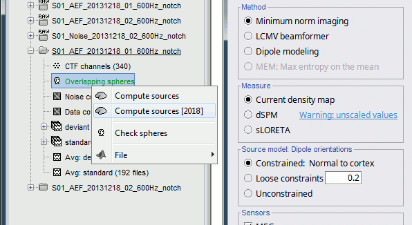
Because we did not request to compute and inverse model for a specific block of recordings, it computed a shared inverse model. If you right-click on this new file, you get a warning message: "Inversion kernel". It does not contain any source map, but only the inverse operator that will allow us to convert the recordings in source maps.
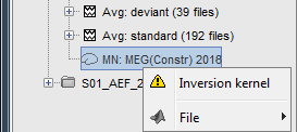
The database explorer now shows one source link to this inverse model for each block of recordings available in this folder, single trials and averages. These links are not real files saved on the hard drive, but you can use them exactly like the first source file we calculated for the deviant average. If you load a link, Brainstorm loads the corresponding the MEG recordings, loads the inverse kernel and multiply the two on the fly before displaying it. This optimized approach saves a lot of computation time and lot of space on the hard drive.
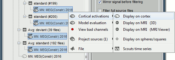
Double-click on the new link for the deviant average, to see what unconstrained source maps look like. The first obvious observation is that the maps look a lot smoother.
![[ATTACH] [ATTACH]](/moin_static1911/brainstorm1/img/attach.png)
We have to be careful with the visual comparisons of constrained and unconstrained source maps displayed on the cortex surface, because they are very different types of data. In unconstrained source maps, we have three dipoles with orthogonal orientations at each cortex location, therefore we cannot represent at once all the information. To display them as an activity map, Brainstorm computes the norm of the vectorial sum of the three orientations at each vertex.

Source map normalization
The current density values returned by the minimum norm method have a few problems:
- They depend a lot on the SNR of the signal, which may vary a lot between different subjects.
- Their amplitude is therefore difficult to interpret directly.
- The values tend to be always higher at the superficy of the brain (close to the sensors).
- The maps are sometimes patchy and difficult to read.
Normalizing the current density maps with respect with a baseline (noise recordings or resting state) can help with all these issues at the same time. Some normalizations can be computed independently from the recordings, and saved as part of the linear source model (dSPM, sLORETA, MNp). An other way of proceeding is to compute a Z-score baseline correction from the current density maps.
All the normalizations options do not change your results, they are just different ways at looking at the same minimum norm maps. If you look at the time series associated with one source, it would be exactly the same for all the normalizations, except for a scaling factor. What changes is only the relative weights between the sources, and these weights do not change over time.
dSPM, sLORETA, MNp
In Run#01, right-click on the average recordings for the deviant stim > Compute sources [2015].
Select sucessively the three normalization options: dSPM, sLORETA, MNp (unconstrained).

Double-click on all of them to compare them:

Current density maps: Tends to highlight the top of the gyri and the superficial sources.
dSPM: Tends to correct that behavior and may give higher values in deeper areas.
sLORETA: produces a very smooth solution where all the potentially activated area of the brain (given to the low spatial resolution of the source localization with MEG/EEG) is shown as connected, regardless of the depth of the sources.
MNp: ???
Z-score
The Z-transformation converts the current density values to a score of deviation from a baseline. For each source separately we define a baseline, compute the average and standard deviation for this segment. Then for every time point we subtract the baseline average and divide by the baseline standard deviation. It tells how much a value deviates from the average at rest (in number of times the standard deviation).
- Drag and drop the unconstrained current density maps (the only link) to the Process1 list.
Run process "Standardize > Z-score normalization", baseline = [-100,-2]ms.
Select the option "Use the norm of the three orientations", if not it would compute the Z-score normalization separately for each direction and then take the norm of the three Z-scored orientation for display, which doesn't make a lot of sense.
The option "dynamic" offers an optimization in the storage of the Z-scored file that can save a lot of disk space in some cases, but that is compatible with the "norm" option for unconstrained sources.
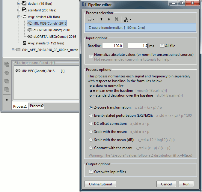
The option "absolute values / norm of the three orientations" caused the call to the intermediate process "Sources > Unconstrained to flat map: norm". This is why the comment of the output file includes the tag "norm".
Note that this process brought down the number of signals in the file from 45,000 (the number of dipoles) to 15,000 (the number of grid points). There is now only one normalized value for each vertex of the cortex surface.
If the baseline and the active state are not in the same file, you can use the Process2 tab: place the baseline in the left list (Files A) and the file to normalize in the right list (Files B).
Delete your experiments
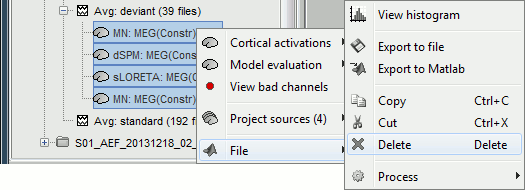
Select all the normalized source maps (everything but the link) and delete them.
Typical recommendations
- Use non-normalized current density maps for:
- Computing shared kernels applied to single trials.
- Averaging single trials across MEG runs.
- Computing time-frequency decompositions or connectivity measures on the single trials.
- Use normalized maps (dSPM, sLORETA, MNp, Z-score) for:
- Estimating the sources for an average response.
- Exploring visually the ERP/ERF at the source level.
- Normalizing the subjects averages before a group analysis.
Average in source space
First compute the same source model for the the second acquisition run.
In Run#02, right-click on the head model or the folder > Compute sources [2015].
Select the options: Minimum norm imaging, Current density map, Unconstrained
Now we have the source maps available for all the trials, we can average them in source space across runs. This allows us to average MEG recordings that were recorded with different head positions (in this case Run#01 and Run#02 have different channel files so they could potentially have different head positions preventing the direct averaging at the sensor level).
- Thanks to the linearity of the minimum norm model, the two following approaches are equivalent:
- Averaging the sources of all the individual trials across runs,
- Averaging the sources for the sensor averages that we already computed for each run. For non-standardized current density maps: MN(Average(trials)) = Average(MN(trials))
- The second solution is a lot faster because it needs to read 4 files (one file per run and per condition) instead of 480 (total number of trials in the two runs).
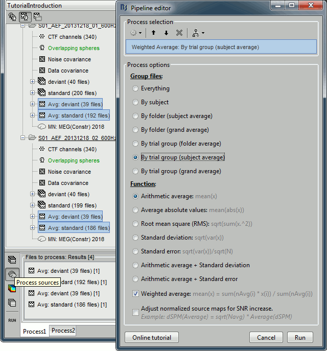
Drag and drop to the Process1 tab the average recordings for Run01 and Run02, then press the [Process sources] button on the left.
Run process "Average > Average files": Select "By trial group (subject average)".
The options "trial group" average together the files that have similar comments.
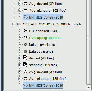
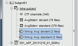
The two averages that are produced (one for each condition) are saved in the folder Intra-subject. This is where all the files that were computed using information from multiple folders within the same subject are going to be saved. If you prefer to have them in different folders, you can always move create new folders and move them there.
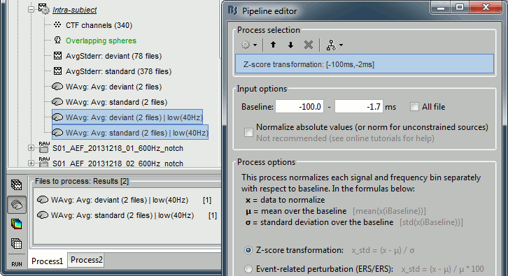
Clear the Process1 list, then drag and drop the new averages in it.
Run process "Standardize > Z-score normalization", baseline = [-100,-2]ms.
Select the option "Use the norm of the three orientations"
Double-click on the source averages to display them (standard=top, deviant=bottom).
You can the average recordings of one or the other run for adding a time reference.
Use the pre-defined view "Left, Right" for looking at the two sides at once (shortcut: "7").
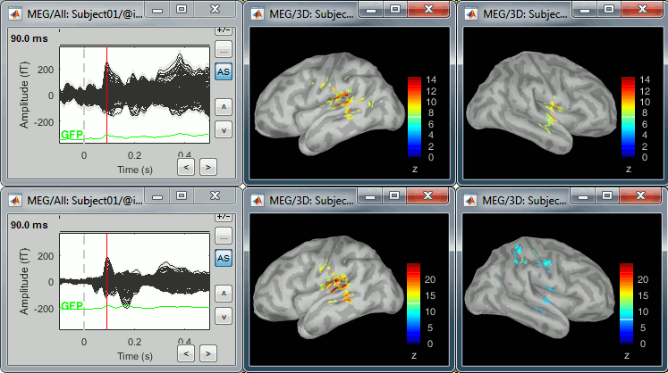
Note that opening the source maps can be very long because of the online filters. Check in the Filter tab, you probably still have a 100Hz low-pass filter applied for the visualization. In the case of averaged source maps, the 15000 source signals are filtered on the fly when you load a source file. This can take a significant amount of time. You may consider unchecking this option if the display is too slow on your computer.
Warning: This approach is valid only for the current density maps. In general, it is not advised to average normalized source maps because the average of the normalized maps is not the same as the normalization of the average. First average, then normalize. This issue is described in an advanced section below.
Display: Contact sheets and movies
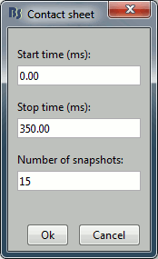
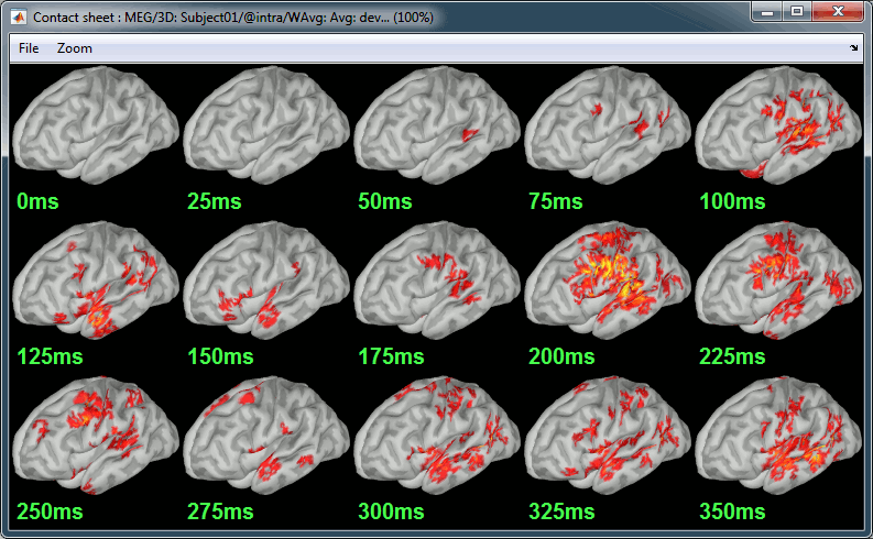
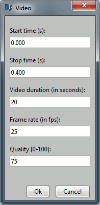
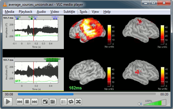
A good way to represent what is happening in time is to generate contact sheets or videos. Right-click on any figure and go to the menu Snapshot to check out all the possible options. For a nicer result, take some time to adjust the size of the figure, the amplitude threshold and the colormap options (hiding the colorbar can be a good option for contact sheets).
A time stamp is added to the captured figure. The size of the text font is fixed, so if you want it to be reable in the contact sheet, you should make you figure very small before starting the capture.
Contact sheet: Right-click on any figure > Snapshot > Time contact sheet: Figure
Movies: Right-click on any figure > Snapshot > Movie (time): All figures (click to download video)
Advanced options
Let's introduce briefly the other options offered for the source estimation. Right-click again on Right / ERF > Compute sources. Click on "Expert mode", you see more options appearing in the window. If you click on Run, you have access to all the options of the wMNE algorithm.
Beamformer options
Dipole fitting options
Output mode
Full results: Saves in one big matrix the values of all the sources (15000) for all the time samples (375). The size in memory of such a matrix is about 45Mb for 300ms of recordings. This is still reasonable, so you may use this option in this case. But if you need to process longer recordings, you may have some "Out of memory" errors in Matlab, or fill your hard drive quickly.
Kernel only: Saves only the Inversion kernel, a matrix that describes how to compute the sources when you know the values at the sensor level. So its size is: number of sources (15000) x number of sensors (151). This is possible because these minimum norm methods are linear methods.
- To get the sources time series, you just need to multiply this kernel by the MEG recordings.
Full results = Inversion kernel * Recordings
- The size of this matrix is about 18Mb. In this case, the difference is not very important because we only process 375 time samples. But this inversion kernel is independent from the recordings length, so you can easily scale its computation to much longer recordings.
Default ?
Probably "Kernel only", as it is faster and produces smaller files.
- All the following operations in Brainstorm will be exactly the same either way. Each time you access the sources values, the program has to do the multiplication Kernel * Recordings, but this is done in a totally transparent way.
The only reason that would make you choose the "Full results" options would be any interest in having the full matrix in one file, in case you want to process the sources values by yourself (filtering, statistics, display...).
Signal properties
Signal to noise ratio (SNR): An estimate of the amplitude SNR of the recordings, as defined in MNE (--snr option in MNE), used to compute the regularization parameter (lambda2 = 1/SNR2). The default value is SNR = 3. Automatic selection of the regularization parameter is currently not supported.
PCA Whitening: Parameter introduced by Rey Ramirez. For more information, see the code of bst_wmne function.
Noise covariance matrix
Full noise covariance: Use the full noise covariance matrix available in Brainstorm database. If the noise covariance file previously computed in is a diagonal matrix (as it is the case in this tutorial), this value is ignored, and the "diagonal noise covariance" option is used instead.
Diagonal noise covariance: Discard the off-diagonal elements of the noise covariance matrix (assuming heteroscedastic uncorrelated noise). Corresponds in MNE to the --diagnoise option.
Regularize noise covariance: Regularize the noise-covariance matrix by the given amount for each type of sensor individually (value is restricted to the range 0...1). For more information, please refer to the MNE manual, section 6.2.4 (options --magreg, --gradreg and --eegreg).
Depth weighting
The minimum-norm estimates have a bias towards superficial currents. This tendency can be alleviated by adjusting these parameters. To understand how to set these parameters, please refer to the MNE manual (options --depth, --weightexp and --weightlimit).
Equations
TODO: John
Rey on sLORETA
Yes in sLORETA the noise covariance is not used at all for the standardization process. It can be used modeling correlated noise and whitening, but that is optional.
I have noticed that a lot of folks are confused about this and I have seen many statements in papers spreading this awful confusion. The sLORETA is standardized by the resolution matrix (diagonal for dipole orientations constraints, or block diagonals for free orientations).
That is why sLORETA has zero localization bias for ALL point-spread functions, and why I always prefer sLORETA over dSPM, MNE, or any beamformer. This is all in the math .... but ..... just so that you know Fas Hsuan Lin's paper comparing sLORETA with dSPM, and MNE has a big mistake, the assumed source covariance matrix is not the identity matrix, and that violates the beauty of the math and results in non-zero localization bias. That's why in Brainstorm the prior source covariance matrix used for sLORETA automatically uses no depth bias compensation (identity matrix). sLORETA accomplishes depth bias compensation via the resolution matrix, NOT via the prior source covariance matrix. Trying to use a depth exponent of 0.7 or 0.8 like we do for MNE and dSPM will mess up sLORETA.You will not find this in a paper, but I checked it all out many years ago. This is critical.
Explain sLORETA units (see email exchanges from Feb 2015)
Issues with dSPM average
Average(dSPM) is NOT equal to dSPM(Average).
There is no problem for the MNE and sLORETA solutions, because the scaling of the noise covariance matrix doesn't impact the results.
    wMNE(Data, NoiseCov) = wMNE(Data, NoiseCov / N)
So when we average we get:
    Average(wMNE(Trials, NoiseCov)) = wMNE(Average, NoiseCov) = wMNE(Average, NoiseCov / N)

But for dSPM we have:
    dSPM(Data, NoiseCov) = dSPM(Data, NoiseCov / N) ./ sqrt(N)
So when we average we get:
    Average(dSPM(Trials, NoiseCov)) = dSPM(Average, NoiseCov) = dSPM(Average, NoiseCov / N) ./ sqrt(N)
Rey: "Basically, the dSPM value at each location is equal to the wMNE value divided by the projection of the estimated noise covariance matrix onto each source point. After whitening, the operational noise covariance matrix is by definition the identity matrix, and hence the projection of the noise is equal to the L2 norm of the row vector of the wMNE inverse operator (in the case of fixed dipole orientations). So, dSPM is what you get when the rows of the wMNE inverse operator all have unit norm (i.e., they all point in different directions but lie in a unit hyper-sphere)."
Rey: "dSPM is really a source mapping of SNR, not of activity. Hence, it's not all so surprising that the single trial SNR maps are smaller...
"Rey: "Perhaps, dSPM should be used only for averaged data (i.e., ERF, ERP), at least until it's all figure out. In a way, dSPM is just MNE followed by the noise normalization. Thus, you could do all the single trial processing with the MNE algorithm, and only do the noise normalization when needed (e.g., after averaging or on single trials only if they are not going to be averaged)."
On the hard drive
Document file tags
Document file structure
Differences for kernel vs. sources
Differences for constrained vs. unconstrained
in_bst_results to get the full sources or apply any process
You can have a look to the corresponding matrix file (right-click > File > View file contents). You would find all the options of forward and inverse modeling, and only one interesting field : ImagingKernel, which contains the inversion kernel. It is a [nVertices x nChannels] matrix that has to be multiplied with the recordings matrix in order to get the activity for each source at all the time samples.
- The minimum norm solution being a linear operation (the time series for each source is a linear combination of all the time series recorded by the sensors), we make this economy of saving only this linear operator instead of the full source matrix (nVertices x nTime)
Links: These links are not saved as files but as specific strings in the database: "link|kernel_file|data_file". This means that to represent them, one should load the shared kernel, load the recordings, and multiply them.
References
Dale AM, Liu AK, Fischl BR, Buckner RL, Belliveau JW, Lewine JD, Halgren E
Dynamic statistical parametric mapping: combining fMRI and MEG for high-resolution imaging of cortical activity. Neuron 2000 Apr, 26(1):55-67Pascual-Marqui RD, Standardized low-resolution brain electromagnetic tomography (sLORETA): technical details, Methods Find Exp Clin Pharmacol 2002, 24 Suppl D:5-12
Additional discussions on the forum
Forum: Minimum norm units (pA.m): http://neuroimage.usc.edu/forums/showthread.php?1246
Forum: Imaging resolution kernels: http://neuroimage.usc.edu/forums/showthread.php?1298
Forum: Spatial smoothing of sources: http://neuroimage.usc.edu/forums/showthread.php?1409
Forum: Units for dSPM and sLORETA: http://neuroimage.usc.edu/forums/showthread.php?1535
Forum: EEG reference: http://neuroimage.usc.edu/forums/showthread.php?1525#post6718
Forum: Sign of the MNE values: http://neuroimage.usc.edu/forums/showthread.php?1649#post7014
Forum: Combining magneto+gradiometers: http://neuroimage.usc.edu/forums/showthread.php?1900
Forum: Residual ocular artifacts: http://neuroimage.usc.edu/forums/showthread.php?1272


