|
Size: 32529
Comment:
|
Size: 32755
Comment:
|
| Deletions are marked like this. | Additions are marked like this. |
| Line 129: | Line 129: |
| A classical way to control the familywise error rate is to replace the p-value threshold with a corrected value, to enforce the expected FWER. The Bonferroni correction sets the significance cut-off at . <<latex($$p\leq\frac{\alpha}{m}$$)>> <<latex($$ \mathit{FWER}\leq\alpha $$)>>. ---- /!\ '''Edit conflict - other version:''' ---- A classical way to control the familywise error rate is to replace the p-value threshold with a corrected value, to enforce the expected FWER. ---- /!\ '''Edit conflict - your version:''' ---- ---- /!\ '''End of edit conflict''' ---- |
A classical way to control the familywise error rate is to replace the p-value threshold with a corrected value, to enforce the expected FWER. The Bonferroni correction sets the significance cut-off at <<latex($$\alpha$$)>>/Ntest. If we set <<latex($$p\leq\alpha}$$)>>/Ntest, then we have <<latex($$ \mathit{FWER}\leq\alpha $$)>>. Following the previous example:<<BR>>'''FWER''' = 1 - prob(no significant results) = 1 - (1 - 0.05/100000)^100000 '''~ 0.0488 < 0.05''' This works well in a context were all the tests are strictly independent. However, in this context the tests have an important level of dependence: two adjacent sensors or time samples always have similar values. In the case of highly correlated tests, the Bonferroni correction tends too be conservative, leading to a high rate of false negatives. |
Tutorial 26: Statistics
[TUTORIAL UNDER DEVELOPMENT: NOT READY FOR PUBLIC USE]
Authors: Francois Tadel, Elizabeth Bock, Dimitrios Pantazis, Richard Leahy, Sylvain Baillet
In this auditory oddball experiment, we would like to test for the significant differences between the brain response to the deviant beeps and the standard beeps, time sample by time sample. Until now we have been computing measures of the brain activity in time or time-frequency domain. We were able to see clear effects or slight tendencies, but these observations were always dependent on an arbitrary amplitude threshold and the configuration of the colormap. With appropriate statistical tests, we can go beyond these empirical observations and assess what are the significant effects in a more formal way.
Contents
- Random variables
- Histograms
- Statistical inference
- Parametric Student's t-test
- Example 1: t-test on recordings
- Correction for multiple comparisons
- STOP READING HERE, EVERYTHING BELOW IS WRONG
- Example 2: t-test on sources
- Permutation tests
- FieldTrip: Non-parametric cluster-based statistic [TODO]
- FieldTrip: Process options [TODO]
- FieldTrip: Example 1 [TODO]
- FieldTrip: Example 2 [TODO]
- Time-frequency files
- One-sided or two-sided
- Workflow: Single subject
- Workflow: Group analysis
- Convert statistic results to regular files
- Export to SPM
- On the hard drive [TODO]
- References
- Additional documentation
- Delete all your experiments
Random variables
In most cases we are interesting in comparing the brain signals recorded for two populations or two experimental conditions A and B.
A and B are two random variables for which we have a limited number of repeated measures: multiple trials in the case of a single subject study, or multiple subject averages in the case of a group analysis. To start with, we will consider that each time sample and each signal (source or sensor) is independent: a random variable represents the possible measures for one sensor/source at one specific time point.
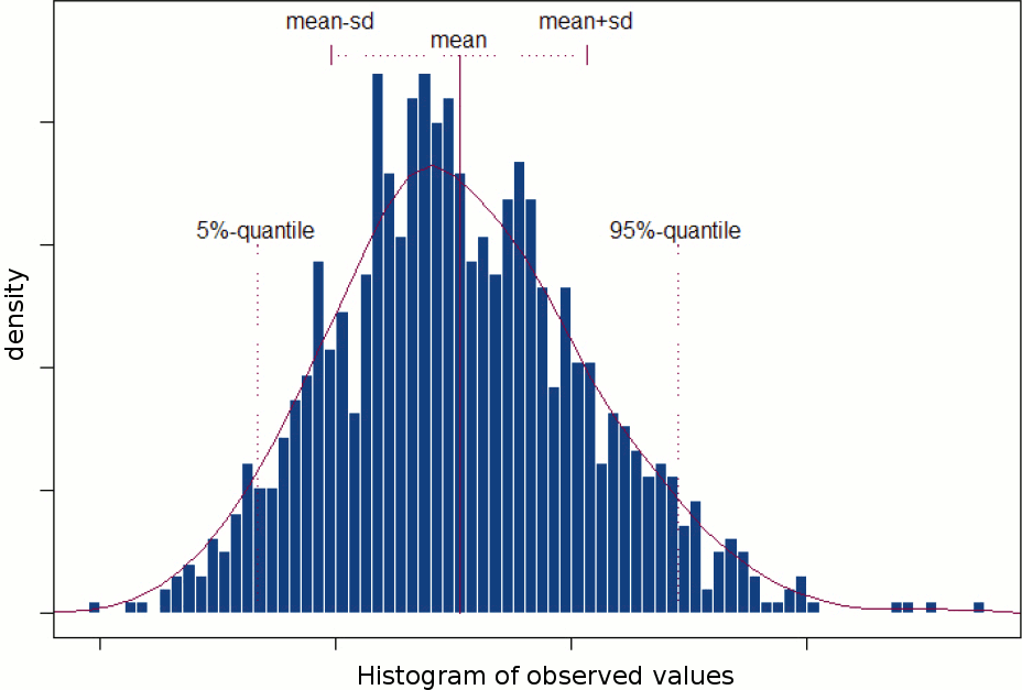
A random variable can be described with its probability distribution: a function which indicates what are the chances to obtain one specific measure if we run the experiment. By repeating the same experiment many times, we can approximate this function with a discrete histogram of observed measures.
Histograms
You can plot histograms like this one in Brainstorm, it may help you understand what you can expect from the statistics functions described in the rest of this tutorial. For instance, seeing a histogram computed with only 4 values would discourage you forever to run any group analysis with 4 subjects...
Recordings
Let's evaluate the recordings we obtained for sensor MLP57, the channel that was showing the highest value at 160ms in the difference of averages computed in the previous tutorial.

We are going to extract only one value for each trial we have imported in the database, and save these values in two separate files, one for each condition (standard and deviant).
In order to observe more meaningful effects, we will process together the trials from the two acquisition runs. As explained in the previous tutorials (#16), this is usually not recommended in MEG analysis, but it can be an acceptable approximation if the subject didn't move between runs.In Process1, select all the deviant trials from both runs.
Run process Extract > Extract values:
Options: Time=[160,160]ms, Sensor="MLP57", Concatenate time (dimension 2)
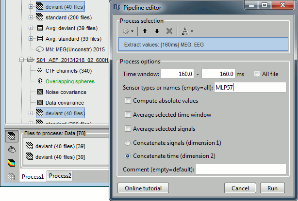
Repeat the same operation for all the standard trials.
You obtain two new files in the folder Intra-subject. If you look inside the files, you can observe that the size of the Value matrix matches the number of trials (78 for deviant, 383 for standard). The matrix is [1 x Ntrials] because we asked to concatenate the extracted values in the 2nd dimension.

To display the distribution of the values in these two files:
select them simultaneously, right-click > File > View histograms.
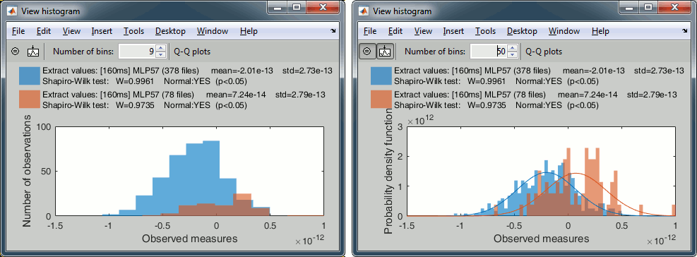
With the buttons in the toolbar, you can edit the way these distributions are represented: number of bins in the histogram, total number of occurances (shows taller bars for standard because it has more values) or density of probability (normalized by the total number of values).
You can additionnally plot the corresponding normal distribution corresponding to the mean μ and standard deviation σ computed from the set of values (using Matlab functions mean and std).When comparing two sample sets A and B, we try to evaluate if the distributions of the measures are equal or not. In most of the questions we explore in EEG/MEG analysis, the distributions are overlapping a lot. The very sparse sampling of the data (a few tens or hundreds repeated measures) doesn't help with the task. Some representations will be more convicing than others to estimate the differences between the two conditions.

Sources (relative)
We can repeat the same operation at the source level and extract all the values for scout A1.
In Process1, select all the deviant trials from both runs. Select button [Process sources].
Run process Extract > Extract scouts time series:
Options: Time=[160,160]ms, Scout="A1", Flip, Concatenate
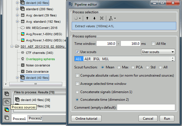
Repeat the same operation for all the standard trials.
Select the two files > Right-click > File > View histogram.
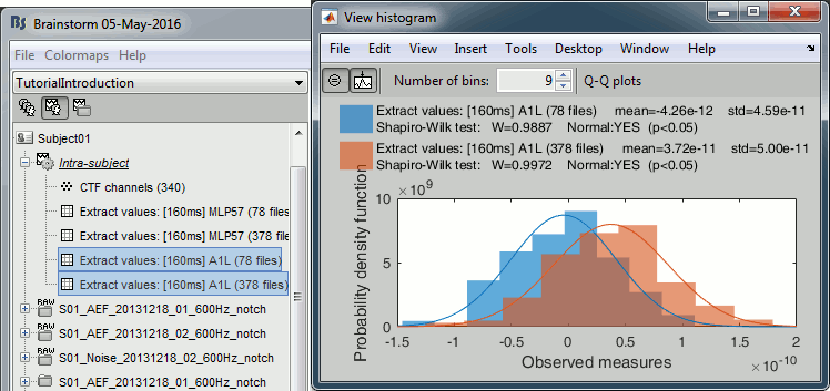
- The distributions still look Gaussian, but the variances are now slightly different. You have to be pay attention to this information when chosing which parametric t-test to run (see below).
Sources (absolute)
In Process1, select the extracted scouts value. Run process "Pre-process > Absolute values".
Display the histograms of the the two rectified files.
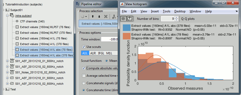
The rectified source values are definitely not following a normal distribution, the shape of the histogram has nothing to do with the corresponding Gaussian curves. As a consequence, if you are using rectified source maps, you will not be able to run independent parametric t-tests.
Additionally, you may have issues with the detection of some effects (see tutorial Difference).
Sources (norm)
When processing unconstrained sources, you are most of the time interested in comparing the norm of the current vector between conditions, rather than the three orientations separately.
To get these values, you can run the process "Sources > Unconstrained to flat maps" on all the trials of both conditions, then to run again the scout values extraction for A1/160ms. This is the distribution you would get if you use the option "Average of absolute values: mean(abs(x))" in the t-test of averaging processes.
![[ATTACH] [ATTACH]](/moin_static1911/brainstorm1/img/attach.png)
Time-frequency
Time-frequency power for recordings: MLP57 / 55ms / 48Hz.

Time-frequency power for sources, Z-score normalized: A1 / 55ms / 48Hz.
![[ATTACH] [ATTACH]](/moin_static1911/brainstorm1/img/attach.png)
- None of these sample sets are distributed following normal distributions. Parametric t-tests in the case of time-frequency power will never be good candidates.
Statistical inference
Hypothesis testing
To show that there is a difference between A and B, we can use a statistical hypothesis test. We start by assuming that the two sets are identical then reject this hypothesis. For all the tests we will use here, the logic is similar:
Define a null hypothesis (H0:"A=B") and alternative hypotheses (eg. H1:"A<B").
- Make some assumptions on the samples we have (eg. A and B are independent, A and B follow normal distributions, A and B have equal variances).
Decide which test is appropriate, and state the relevant test statistic T (eg. Student t-test).
Compute from the measures (Aobs, Bobs) the observed value of the test statistic (tobs).
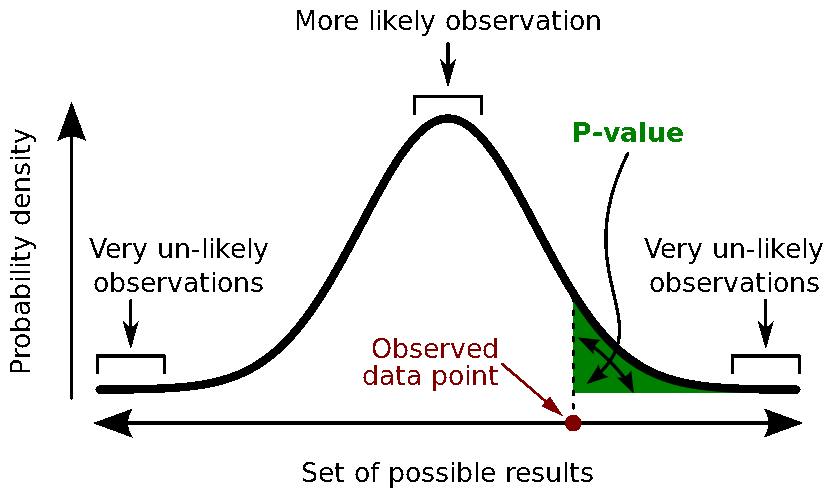
Calculate the p-value. This is the probability, under the null hypothesis, of sampling a test statistic at least as extreme as that which was observed. A value of (p<0.05) for the null hypothesis has to be interpreted as follows: "If the null hypothesis is true, the chance that we find a test statistic as extreme or more extreme than the one observed is less than 5%".
Reject the null hypothesis if and only if the p-value is less than the significance level threshold (α).
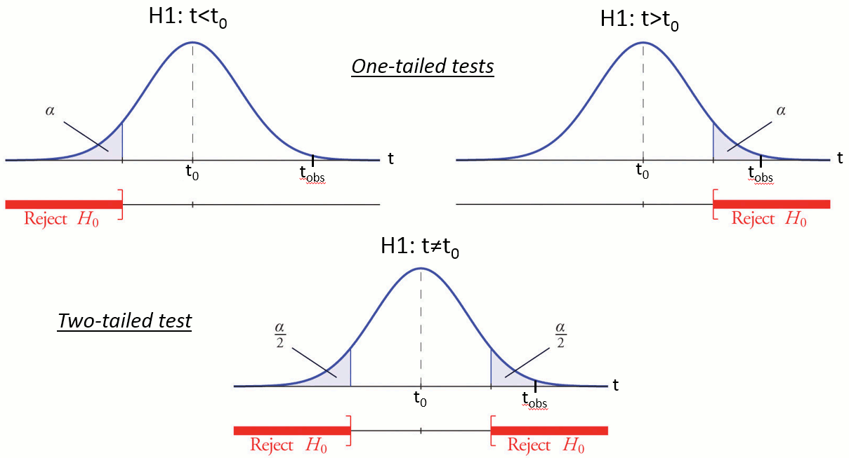
Evaluation of a test
The quality of test can be evaluated based on two criteria:
Sensitivity: True positive rate = power = ability to correctly reject the null hyopthesis and control for the false negative rate (type II error rate). A very sensitive test detects a lot of significant effects, but with a lot of false positive.
Specificity: True negative rate = ability to correctly accept the null hypothesis and control for the false positive rate (type I error rate). A very specific test detects only the effects that are clearly non-ambiguous, but can be too conservative and miss a lot of the effects of interest.
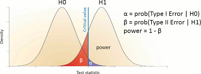
Different categories of tests
Two families of tests can be helpful in our case: parametric and non-parametric tests.
Parametric tests need some strong assumptions on the probability distributions of A and B then use some well-known properties of these distributions to compare them, based on a few simple parameters (typically the mean and variance). The examples which will be described here are the Student's t-tests.
Non-parametric tests only rely on the measured data, but are lot more computationally intensive.
Parametric Student's t-test
Assumptions
The Student's t-test is a widely-used parametric test to evaluate the difference between the means of two random variables (two-sample test), or between the mean of one variable and one known value (one-sample test). If the assumptions are correct, the t-statistic follows a Student's t-distribution.
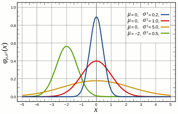
The main assumption for using a t-test is that the random variables involved follow a normal distribution (mean: μ, standard deviation: σ). The figure below shows a few example of normal distributions.
t-statistic
Depending on the type of data we are testing, we can have different variants for this test:
One-sample t-test (testing against a known mean μ0):

where is the sample mean, σ is the sample standard deviation and n is the sample size.
 Dependent t-test for paired samples (eg.when testing two conditions across subject). Equivalent to testing the difference of the pairs of samples against zero with a one-sample t-test:

where D=A-B, is the average of D and σD its standard deviation.
 Independent two-sample test, equal variance (equal or unequal sample sizes):

where and
and  are the unbiased estimators of the variances of the two samples.
 Independent two-sample test, unequal variance (Welch's t-test):

where and
and  are the sample sizes of A and B.
p-value
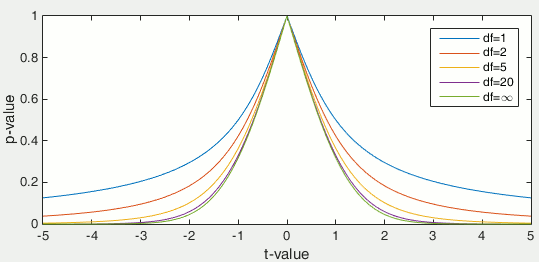
Once the t-value is computed (tobs in the previous section), we can convert it to a p-value based on the known distributions of the t-statistic. This conversion depends on two factors: the number of degrees of freedom and the tails of the distribution we want to consider. For a two-tailed t-test, the two following commands in Matlab are equivalent and can convert the t-values in p-values.
To obtain the p-values for a one-tailed t-test, you can simply divide the p-values by 2.
p = betainc(df./(df + t.^2), df/2, 0.5);    % Without the Statistics toolbox
p = 2*(1-tcdf(abs(t),df));                  % With the Statistics toolbox
The distribution of this function for different numbers of degrees of freedom:
Example 1: t-test on recordings
Parametric t-tests require the values tested to follow a normal distribution. The recordings evaluated in the histograms sections above (MLP57/160ms) show distributions that are matching relatively well this assumption: the shape of the histogram follows the trace of the corresponding normal function, and with very similar variances. It looks reasonable to use a parametric t-test in this case.
In the Process2 tab, select the following files, from both runs (approximation discussed above):
Files A: All the deviant trials, with the [Process recordings] button selected.
Files B: All the standard trials, with the [Process recordings] button selected.
Run the process "Test > Parametric t-test", Equal variance, Arithmetic average.
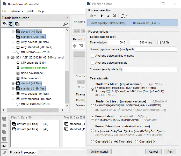
Double-click on the new file for displaying it. With the new tab "Stat" you can control the p-value threshold and the correction you want to apply for multiple comparisons (see next section).

Correction for multiple comparisons
Multiple comparison problem
The approach described in this first example performs many tests simulateneously. We test independently each MEG sensor and each time sample across the trials, so we run a total of 274*361 = 98914 t-tests.
If we select a critical value of 0.05 (p<0.05), it means that we want to see what is significantly different between the conditions while accepting the risk to observe a false positive in 5% of the cases. If we run around 100,000 times the test, we can expect to observe around 5,000 false positives. We need to control better for false positives when dealing with multiple tests.
The probability to observe at least one false positive, or familywise error rate (FWER) is almost 1:
FWER = 1 - prob(no significant results) = 1 - (1 - 0.05)^100000 ~ 1
Bonferroni correction
A classical way to control the familywise error rate is to replace the p-value threshold with a corrected value, to enforce the expected FWER. The Bonferroni correction sets the significance cut-off at  /Ntest. If we set
latex error! exitcode was 1 (signal 0), transscript follows:

This is pdfTeX, Version 3.141592653-2.6-1.40.22 (TeX Live 2022/dev/Debian) (preloaded format=latex)
entering extended mode
(./latex_205784928bf43bb6da612d256d3eff119dfd36b3_p.tex
LaTeX2e <2021-11-15> patch level 1
L3 programming layer <2022-01-21>
(/usr/share/texlive/texmf-dist/tex/latex/base/article.cls
Document Class: article 2021/10/04 v1.4n Standard LaTeX document class
(/usr/share/texlive/texmf-dist/tex/latex/base/size12.clo))
(/usr/share/texlive/texmf-dist/tex/latex/base/inputenc.sty)
(/usr/share/texlive/texmf-dist/tex/latex/l3backend/l3backend-dvips.def)
No file latex_205784928bf43bb6da612d256d3eff119dfd36b3_p.aux.
! Extra }, or forgotten $.
l.7 $$p\leq\alpha}
                  $$
[1] (./latex_205784928bf43bb6da612d256d3eff119dfd36b3_p.aux) )
(see the transcript file for additional information)
Output written on latex_205784928bf43bb6da612d256d3eff119dfd36b3_p.dvi (1 page,
 296 bytes).
Transcript written on latex_205784928bf43bb6da612d256d3eff119dfd36b3_p.log.
/Ntest, then we have  . Following the previous example:
FWER = 1 - prob(no significant results) = 1 - (1 - 0.05/100000)^100000 ~ 0.0488 < 0.05
This works well in a context were all the tests are strictly independent. However, in this context the tests have an important level of dependence: two adjacent sensors or time samples always have similar values. In the case of highly correlated tests, the Bonferroni correction tends too be conservative, leading to a high rate of false negatives.
STOP READING HERE, EVERYTHING BELOW IS WRONG
Example 2: t-test on sources
Parametric method require the values tested to follow a Gaussian distribution. Some sets of data could be considered as Gaussian (example: screen capture of the histogram of the values recorded by one sensor at one time point), some are not (example: histogram ABS(values) at one point).
WARNING: This parametric t-test is valid only for constrained sources. In the case of unconstrained sources, the norm of the three orientations is used, which breaks the hypothesis of the tested values following a Gaussian distribution. This test is now illustrated on unconstrained sources, but this will change when we figure out the correct parametric test to apply on unconstrained sources.
- In the Process2 tab, select the following files:
Files A: All the deviant trials, with the [Process sources] button selected.
Files B: All the standard trials, with the [Process sources] button selected.
Run the process "Test > Student's t-test", Equal variance, Absolute value of average.
This option will convert the unconstrained source maps (three dipoles at each cortex location) into a flat cortical map by taking the norm of the three dipole orientations before computing the difference.
![[ATTACH] [ATTACH]](/moin_static1911/brainstorm1/img/attach.png)
Double-click on the new file for displaying it. With the new tab "Stat" you can control the p-value threshold and the correction you want to apply for multiple comparisons (see next section).
![[ATTACH] [ATTACH]](/moin_static1911/brainstorm1/img/attach.png)
Set the options in the Stat tab: p-value threshold: 0.05, Multiple comparisons: Uncorrected.
What we see in this figure are the t-values corresponding to p-values under the threshold. We can make similar observations than with the difference of means, but without the arbitrary amplitude threshold (this slider is now disabled in the Surface tab). If at a given time point a vertex is red in this view, the mean of the deviant condition is significantly higher than the standard conditions (p<0.05).
![[ATTACH] [ATTACH]](/moin_static1911/brainstorm1/img/attach.png)
This approach considers each time sample and each surface vertex separately. This means that we have done Nvertices*Ntime = 15002*361 = 5415722 t-tests. The threshold at p<0.05 controls correctly for false positives at one point but not for the entire cortex. We need to correct the p-values for multiple comparisons. The logic of two types of corrections available in the Stat tab (FDR and Bonferroni) is explained in Bennett et al (2009).
Select the correction for multiple comparison "False discovery rate (FDR)". You will see that a lot less elementrs survive this new threshold. In the Matlab command window, you can see the average corrected p-value, that replace for each vertex the original p-threshold (0.05):
BST> Average corrected p-threshold: 0.000315138 (FDR, Ntests=5415722)From the Scout tab, you can also plot the scouts time series and get in this way a summary of what is happening in your regions of interest. Positive peaks indicate the latencies when at least one vertex of the scout has a value that is significantly higher in the deviant condition. The values that are shown are the averaged t-values in the scout.
![[ATTACH] [ATTACH]](/moin_static1911/brainstorm1/img/attach.png)
Permutation tests
Permutation test: https://en.wikipedia.org/wiki/Resampling_%28statistics%29
FieldTrip: Non-parametric cluster-based statistic [TODO]
We have the possibility to call some of the FieldTrip functions from the Brainstorm environment. For this, you need first to install the FieldTrip toolbox on your computer and add it to your Matlab path.
For a complete description of non-parametric cluster-based statistics in FieldTrip, read the following article: Maris & Oostendveld (2007). Additional information can be found on the FieldTrip website:
Tutorial: Parametric and non-parametric statistics on event-related fields
Tutorial: Cluster-based permutation tests on event related fields
Tutorial: Cluster-based permutation tests on time-frequency data
Tutorial: How NOT to interpret results from a cluster-based permutation test
Video: Statistics using non-parametric randomization techniques
Video: Non-parametric cluster-based statistical testing of MEG/EEG data
Functions: ft_timelockstatistics, ft_sourcestatistics, ft_freqstatistics
Permuation-based non-parametric statistics are more flexible and do not require to do any assumption on the distribution of the data, but on the other hand they are a lot more complicated to process. Calling FieldTrip's function ft_sourcestatistics requires a lot more memory because all the data has to be loaded at once, and a lot more computation time because the same test is repeated many times.
Running this function in the same way as the parametric t-test previously (full cortex, all the trials and all the time points) would require 45000*461*361*8/1024^3 = 58 Gb of memory just to load the data. This is impossible on most computers, we have to give up at least one dimension and run the test only for one time sample or one region of interest.
FieldTrip: Process options [TODO]
Screen captures for the two processes:
Description of the process options:
The options available here match the options passed to the function ft_sourcestatistics.
Cluster correction: Define what a cluster is for the different data types (recordings, surface source maps, volume source models, scouts)
Default options:
- clusterstatistic = 'maxsum'
- method = 'montecarlo'
- correcttail = 'prob'
FieldTrip: Example 1 [TODO]
We will run this FieldTrip function first on the scouts time series and then on a short time window.
- Keep the same selection in Process2: all the deviant trials in FilesA, all the standard trials in FilesB.
Run process: Test > FieldTrip: ft_sourcestatistics, select the options as illustrated below.
![[ATTACH] [ATTACH]](/moin_static1911/brainstorm1/img/attach.png)
Double-click on the new file to display it:
- Display on the cortex: see section "Convert statistic results to regular files" below
FieldTrip: Example 2 [TODO]
short time window
Time-frequency files
Both ft_sourcestatistics and ft_freqstatistics are available.
Use ft_sourcestatistics if the input files contain full source maps, and ft_freqstatistics for all the other cases (scouts or sensors).
One-sided or two-sided
two-tailed test on either (A-B) or (|A|-|B|)
The statistic, after thresholding should be displayed as a bipolar signal (red – positive, blue – negative) since this does affect interpretation
Constrained (A-B), null hypothesis H0: A=B, We compute a z-score through normalization using a pre-stim period and apply FDR-controlled thresholding to identify significant differences with a two tailed test.
Constraine (|A|-|B|), null hypothesis H0: |A|=|B|, We compute a z-score through normalization using a pre-stim period and apply FDR-controlled thresholding to identify significant differences with a two tailed test.
Unconstrained RMS(X-Y), H0: RMS(X-Y)=0, Since the statistic is non-negative a one-tailed test is used.
Unconstrained (RMS(X) –RMS(Y)), H0: RMS(X)-RMS(Y)=0, we use a two-tailed test and use a bipolar display to differentiate increased from decreased amplitude.
Workflow: Single subject
You want to test for one unique subject what is significantly different between two experimental conditions. You are going to compare the single trials corresponding to each condition directly.
This is the case for this tutorial dataset, we want to know what is different between the brain responses to the deviant beep and the standard beep.
Sensor recordings: Not advised for MEG with multiple runs, correct for EEG.
Parametric t-test: Correct
- Select the option "Arithmetic average: mean(x)".
- No restriction on the number of trials.
Non-parametric t-test: Correct
- Do not select the option "Test absolute values".
- No restriction on the number of trials.
Difference of means:
- Select the option "Arithmetic average: mean(x)".
- Use the same number of trials for both conditions.
Constrained source maps (one value per vertex):
- Use the non-normalized minimum norm maps for all the trials (no Z-score).
Parametric t-test: Incorrect
- Select the option "Absolue value of average: abs(mean(x))".
- No restriction on the number of trials.
Non-parametric t-test: Correct
- Select the option "Test absolute values".
- No restriction on the number of trials.
Difference of means:
- Select the option "Absolue value of average: abs(mean(x))".
- Use the same number of trials for both conditions.
Unconstrainted source maps (three values per vertex):
Parametric t-test: Incorrect
- ?
Non-parametric t-test: Correct
- ?
Difference of means:
- ?
Time-frequency maps:
- Test the non-normalized time-frequency maps for all the trials (no Z-score or ERS/ERD).
Parametric t-test: ?
- No restriction on the number of trials.
Non-parametric t-test: Correct
- No restriction on the number of trials.
Difference of means:
- Use the same number of trials for both conditions.
Workflow: Group analysis
You have the same two conditions recorded for multiple subjects.
Sensor recordings: Strongly discouraged for MEG, correct for EEG.
- For each subject: Compute the average of the trials for each condition individually.
- Do not apply an absolute value.
- Use the same number of trials for all the subjects.
- Test the subject averages.
- Do no apply an absolute value.
Source maps (template anatomy):
- For each subject: Average the non-normalized minimumn norm maps for the trials of each condition.
- Use the same number of trials for all the subjects.
If you can't use the same number of trials, you have to correct the Z-score values [TODO].
- Normalize the averages using a Z-score wrt with a baseline.
- Select the option: "Use absolue values of source activations"
- Select the option: "Dynamic" (does not make any difference but could be faster).
- Test the normalized averages across subjects.
- Do not apply an absolute value.
Source maps (individual anatomy):
- For each subject: Average the non-normalized minimumn norm maps for the trials of each condition.
- Use the same number of trials for all the subjects.
If you can't use the same number of trials, you have to correct the Z-score values [TODO].
- Normalize the averages using a Z-score wrt with a baseline.
- Select the option: "Use absolue values of source activations"
- Select the option: "Dynamic" (does not make any difference but could be faster).
- Project the normalized maps on the template anatomy.
- Option: Smooth spatially the source maps.
- Test the normalized averages across subjects.
- Do not apply an absolute value.
Time-frequency maps:
- For each subject: Compute the average time-frequency decompositions of all the trials for each condition (using the advanced options of the "Morlet wavelets" and "Hilbert transform" processes).
- Use the same number of trials for all the subjects.
- Normalize the averages wrt with a baseline (Z-score or ERS/ERD).
- Test the normalized averages across subjects.
- Do no apply an absolute value.
Convert statistic results to regular files
Process: Extract > Apply statistc threshold
Process: Simulate > Simulate recordings from scout [TODO]
Export to SPM
An alternative to running the statical tests in Brainstorm is to export all the data and compute the tests with an external program (R, Matlab, SPM, etc). Multiple menus exist to export files to external file formats (right-click on a file > File > Export to file).
Two tutorials explain to export data specifically to SPM:
Export source maps to SPM8 (volume)
Export source maps to SPM12 (surface)
On the hard drive [TODO]
Right click one of the first TF file we computed > File > View file contents.
Useful functions
- process_ttest:
- process_ttest_paired:
- process_ttest_zero:
- process_ttest_baseline:
References
Bennett CM, Wolford GL, Miller MB, The principled control of false positives in neuroimaging
Soc Cogn Affect Neurosci (2009), 4(4):417-422.Maris E, Oostendveld R, Nonparametric statistical testing of EEG- and MEG-data
J Neurosci Methods (2007), 164(1):177-90.Maris E, Statistical testing in electrophysiological studies
Psychophysiology (2012), 49(4):549-65Pantazis D, Nichols TE, Baillet S, Leahy RM. A comparison of random field theory and permutation methods for the statistical analysis of MEG data, Neuroimage (2005), 25(2):383-94.
FieldTrip video: Non-parametric cluster-based statistical testing of MEG/EEG data:
https://www.youtube.com/watch?v=vOSfabsDUNg
Additional documentation
Forum: Multiple comparisons: http://neuroimage.usc.edu/forums/showthread.php?1297
Forum: Cluster neighborhoods: http://neuroimage.usc.edu/forums/showthread.php?2132
Forum: Differences FieldTrip-Brainstorm: http://neuroimage.usc.edu/forums/showthread.php?2164
Delete all your experiments
Before moving to the next tutorial, delete all the statistic results you computed in this tutorial. It will make the database structure less confusing for the following tutorials.


