|
Size: 9995
Comment:
|
Size: 21160
Comment:
|
| Deletions are marked like this. | Additions are marked like this. |
| Line 1: | Line 1: |
| = Import and process Neuromag raw recordings = This tutorial describes how to process raw Neuromag recordings. It is based on median nerve stimulation acquired at MGH in 2005 with a Neuromag Vectorview 306 system. The sample dataset contains the results for one subject for both arms. |
= Elekta-Neuromag recordings = This tutorial describes how to process continuous Elekta-Neuromag MEG recordings. It is based on median nerve stimulation acquired at the Massachusetts General Hospital in 2005 with a Neuromag Vectorview 306 system. The sample dataset contains the results for one subject for both arms: 18 minutes, 300 stimulations per arm. |
| Line 4: | Line 4: |
| This document shows what to do step by step, but does not really explain what is happening, the meaning of the different options or processes, the issues or bugs you can encounter, and does not provide an exhaustive description of the software features. Those topics are introduced in the basic tutorials based on CTF recordings; so make sure that you followed all those initial tutorials before going through this one. | Note that the operations used here are not detailed, the goal of this tutorial is not to introduce Brainstorm to new users. For in-depth explanations of the interface and theoretical foundations, please refer to the [[http://neuroimage.usc.edu/brainstorm/Tutorials#Get_started|introduction tutorials]]. |
| Line 6: | Line 6: |
| The script file '''tutorial_mind_neuromag.m''' in the brainstorm3/toolbox/script folder performs exactly the same tasks automatically, without any user interaction. Please have a look at this file if you plan to write scripts to process recordings in .fif format. | <<TableOfContents(3,2)>> |
| Line 8: | Line 8: |
| <<TableOfContents(2)>> | <<Include(DatasetMedianNerveNeuromag, , from="\<\<HTML\(\<!-- START-PAGE --\>\)\>\>", to="\<\<HTML\(\<!-- STOP-SHORT --\>\)\>\>")>> |
| Line 11: | Line 11: |
| * It is considered that you followed all the basic tutorials and that you already have a fully working copy of Brainstorm installed on your computer. * Go to the [[http://neuroimage.usc.edu/brainstorm3_register/download.php|Download]] page of this website, and dowload the file "bst_sample_mind_neuromag.zip". * Unzip it in a folder that is not in any of the Brainstorm folders (program folder or database folder). This is really important that you always keep your original data files in a separate folder: the program folder can be deleted when updating the software, and the contents of the database folder is supposed to be manipulated only by the program itself. |
* '''Requirements''': You have already followed all the basic tutorials and you have a working copy of Brainstorm installed on your computer. * Go to the [[http://neuroimage.usc.edu/bst/download.php|Download]] page of this website and download the file '''sample_neuromag.zip''' * Unzip it in a folder that is not in any of the Brainstorm folders (program folder or database folder) |
| Line 15: | Line 15: |
| * In the protocols drop-down list, select the menu "Create new protocol". | * Menu File > Create new protocol > '''TutorialNeuromag''', with the following options: * '''No, use individual anatomy''', * '''No, use one channel file per run'''.<<BR>><<BR>> {{attachment:createProtocol.gif||height="372",width="347"}} |
| Line 17: | Line 19: |
| * Name it "!TutorialNeuromag", and select all the options as illustrated: No default anatomy, Use individual anatomy, Use one channel file per subject (we have only one run, it's possible to share the channels positions and head models between diffrerent conditions).<<BR>><<BR>> {{attachment:createProtocol.gif}} | == Import the anatomy == * Right-click on the TutorialNeuromag folder > New subject > Subject01 (leave all the defaults).<<BR>><<BR>> {{attachment:createSubjectMenu.gif||height="165",width="343"}} {{attachment:createSubject.gif||height="309",width="296"}} * Right-click on the subject node > Import anatomy folder: * Set the file format: "FreeSurfer folder" * Select the folder: '''sample_neuromag/anatomy''' * Number of vertices of the cortex surface: 15000 (default value) <<BR>><<BR>> {{attachment:mriImportMenu.gif||height="224",width="180"}} {{attachment:mriFile.gif||height="167",width="362"}} * Set the 6 required fiducial points (indicated in MRI coordinates): * NAS: x=131, y=232, z=123 * LPA: x=48, y=136, z=74 * RPA: x=204, y=131, z=67 * AC: x=127, y=143, z=118 * PC: x=127, y=117, z=111 * IH: x=127, y=120, z=167 (anywhere on the midsagittal plane) * At the end of the process, make sure that the file "cortex_15000V" is selected (downsampled pial surface, that will be used for the source estimation). If it is not, double-click on it to select it as the default cortex surface.<<BR>><<BR>> {{attachment:anatomy.gif||height="248",width="400"}} |
| Line 19: | Line 34: |
| == Importing anatomy == === Create the subject === * Select the "Anatomy" exploration mode (first button in the toolbar above the database explorer). * Right-click on the protocol node and select "New subject".<<BR>><<BR>> {{attachment:createSubjectMenu.gif}} * You can leave the default name "Subject01" and the default options. Then click on Save.<<BR>><<BR>> {{attachment:createSubject.gif}} |
== Access the recordings == === Link the FIF file to the database === * The sample_neuromag package contains one run for one subject only. * Switch to the "functional data" view, the middle button in the toolbar above the database explorer. * Right click on the Subject01 > Review raw file: <<BR>><<BR>> {{attachment:reviewMenu.gif||height="159",width="210"}} {{attachment:reviewFile.gif||height="160",width="427"}} * Select the file format: '''MEG/EEG Neuromag FIFF (*.fif)''' * Pick the file: '''sample_neuromag/data/mind004_050924_median01_raw.fif''' * Select "Event channel" when asked about the events.<<BR>><<BR>> {{attachment:eventsImport.gif||height="157",width="280"}} * Then you have to select from which technical tracks you want to read the events. <<BR>><<BR>> {{attachment:eventsChannels.gif||height="165",width="375"}} * In this dataset, the tracks of interest are: * '''STI 001''': Contains the onsets of the electric stimulation of the '''right '''arm. * '''STI 002''': Contains the onsets of the electric stimulation of the '''left '''arm. * These are not standard settings, they depend on your acquisition setup. In most cases, you would rather import "events" defined with the Neuromag acquisition software, which are saved in tracks STI 014, STI 101, STI 201... * Select '''STI 001''' and '''STI 002'''. The full tracks are read, all the changes of values are detected from these two tracks and a list of events is created. * At the end, you're asked if you want to "Refine the registration with the head points". This operation improves the initial MRI/MEG registration by fitting the head points digitized at the MEG acquisition and the scalp surface. Answer '''YES'''.<<BR>><<BR>> {{attachment:refine.gif||height="170",width="324"}} <<BR>> * Always make sure that the final registration looks good. The yellow surface represents the inner surface of the MEG helmet and the green dots represent the head points that were saved with the MEG recordings. In this case the registration looks acceptable. If you consider it is not the case, you can fix it manually: right-click on the channel file > MRI registration > Edit. <<BR>><<BR>> {{attachment:checkRegistrationFig.gif||height="199",width="218"}} |
| Line 25: | Line 51: |
| === Import the MRI === * Right-click on the subject node, and select "Import MRI". Select the file: sample_mind_neuromag/anatomy/T1.mri<<BR>><<BR>> {{attachment:mriImportMenu.gif}} {{attachment:mriFile.gif}} * The orientation of the MRI is already ok, you just have to mark all the six fiducial points, as explained in the following wiki page: [[CoordinateSystems|Coordinate systems]]. Click on save button when you're done.<<BR>><<BR>> {{attachment:fiducials.gif}} * If at some point you do not see the files you've just imported in the database explorer, you just need to refresh the display: by pressing F5, or using the menu File > Refresh tree display. === Import the surfaces === * Right-click again on the subject node, and select "Import surfaces". Select the "!FreeSurfer surfaces" file type, and select all the surface files at once, holding the SHIFT or CTRL buttons. Click on Open.<<BR>><<BR>> {{attachment:surfaceFiles.gif}} * Answer "Yes" to the question "Align surfaces with MRI now?". You should see the following nodes in the database.<<BR>><<BR>> {{attachment:surfListInit.gif}} * "outer skin" = Head, used for surfaces/MRI registration * "inner skull" = Internal surface of the skull, used for the computation of the "overlapping spheres" forward model * "lh" = Left hemisphere * "rh" = Right hemisphere * "pial" = External cortical surface = grey matter/CSF interface (used for source estimation) * "white" = External white matter surface = interface between the grey and the white matter (not used in this tutorial) * Downsample the two pial and the two white surfaces to 7,500 vertices each (right-click > Less vertices) * Merge the two downsampled hemispheres of the pial surface (select both lh.pial_7500 and rh.pial_7500 files, right-click > Merge surfaces). Rename the new surface in "cortex". * Do the same with the white matter. Call the result "white". * Delete all the intermediate lh and rh surfaces. Rename the head and the inner skull with shorter names. Display all the surfaces and play with the colors and transparency to check that everything what imported correctly. You should obtain something like this:<<BR>><<BR>> {{attachment:surfListFinal.gif}} {{attachment:surfTest.gif}} == Importing MEG recordings == * Select the "Functional data / sorted by subject" exploration mode (second button in the toolbar above the database explorer). * Right click on the subject, select Import MEG/EEG. Select the "Neuromag FIFF" file type, and open the only .fif file in the folder sample_mind_neuromag/data.<<BR>><<BR>> {{attachment:megImportMenu.gif}} * Select "Event channel" when asked about the events.<<BR>><<BR>> {{attachment:eventsImport.gif}} * You have then to select from which technical track you want to read the events. <<BR>><<BR>> {{attachment:eventsChannels.gif}} * In this dataset, the tracks of interest are: * STI 001: Contains the onsets of the electric stimulation of the '''right '''arm. * STI 002: Contains the onsets of the electric stimulation of the '''left '''arm. * Those are not standard settings, they depend on your acquisition setup. In most cases, you would rather import "events" defined with the Neuromag acquisition software, which are saved in tracks STI 014, STI 101, STI 201... * Click on "STI 001". The full track is read, all the changes of values are extracted and a list of events is created. * Answer "No" when asked whether to save this list of events. This would create a .eve file in the same folder, that would be read instead of the stimulation channel during later access to the raw .fif file. It would provide a much faster access to the events present in the track "STI 001", but we do not need that, because we will have to import the events of the "STI 002". * The following figure appears, that asks how to import those recordings in the Brainstorm database.<<BR>><<BR>> {{attachment:importOptions.gif}} * __Time window__: Time range of interest. Now we want to keep the whole time definition, we are interested by all the stimulations. * __Split__: Useful to import continuous recordings without events. We do not need this here. * __Events selection__: Check the "Use events" option, and select "Event #5". * The value between parenthesis represents the number of occurrences of this event. * Event #5 represents the instants where the value of track STI 001 changing from 0 to 5 (electric stimulation) * Event #0 is set when the value goes back to zero * __Epoch time__: Time instants that will be extracted before an after each event, to create the epochs that will be saved in the database. Set it to [-100, +300] ms * __Use Signal Space Projections__: Save and use the SSP vectors created by !MaxFilter or during other pre-processing steps. Keep this option selected. * __Remove DC Offset__: Check this option, and select: Time range: [-100, 0] ms. <<BR>>For each epoch, this will: compute the average of each channel over the baseline (pre-stimulus interval: -100ms to 0ms), and subtract it from the channel at all the times in [-100,+300]ms. * __Resample recordings__: Keep this unchecked * __Create new conditions for epochs__: If selected, a new condition is created for each event type (here, it will create a condition "Event_5"). If not selected, all the epochs from all the selected events are saved in the same condition, the one that was selected in the database explorer (if no condition selected, create a condition called "New condition"). * Click on Import and wait. * At the end, you get something like this:<<BR>><<BR>> {{attachment:treeAfterImport1.gif}} * Rename the condition "Event_5" into "Right" (Right-click > Rename, or press F2, or click twice waiting a while before the two clicks). * Repeat all those steps to import the events from track "STI 002". Rename "Event_5" into "Left". Your database should look like this:<<BR>><<BR>> {{attachment:treeAfterImport2.gif}} * __Note__: if you do not rename the condition "Event_5" in "Right" between the two imports, you would have at the end all the epochs in the same Event_5 condition. In this case, another way (and maybe safer) way to proceed is to: * Create two conditions Left and Right before starting to import the recordings. * Import the "STI 001" events in condition Right, and the "STI 002" in Left (do not forget to uncheck the option "Create new conditions for epochs", if not the condition selection would be overridden) |
=== Review the recordings === * Right-click on the "Link to raw file" to see what types of channels are available:<<BR>><<BR>> {{attachment:listTypes.gif||height="341",width="332"}} * '''MEG (all)''': Represents all the MEG sensors in the file (magnetometers and gradiometers) * '''MEG (magnetometers)''': 101 magnetometers (sensor names ending with a "1") * '''MEG (gradiometers)''': 202 planar gradiometers (sensor names ending with "2" or "3") * '''ECG''': Electro-cardiogram * '''EOG''': Electro-oculogram * '''Stim''': All the stimulation lines * Double-click on the file to display all the MEG sensors. * In the Record tab, look at the list of the available default display configurations for the Neuromag Vectorview MEG systems. If you would like to use different combinations of sensors, you can create your own combinations with the entry "Edit montages..."<<BR>><<BR>> {{attachment:montages.gif||height="333",width="457"}} |
| Line 76: | Line 63: |
| === Stimulation artifact removal === The electric stimulation of the median nerve induces a strong artefact right after 0ms. We are going to use a simple trick to remove this artifact: re-interpolate the values between 0ms and 4ms (linear interpolation). It doesn't affect much the data but will make all the displays much better. |
=== Evaluate the recordings === * Drag and drop the "Link to raw file" into the Process1 list. * Select the process "'''Frequency > Power spectrum density'''", configure it as follows:<<BR>><<BR>> {{attachment:processPsd.gif||height="358",width="487"}} * In all the processes, the types of sensors can be specified using the following convention: * '''MEG''': All the MEG sensors * '''MEG MAG''': All the magnetometers * '''MEG GRAD''': All the gradiometers * '''MEG GRAD2''': Only the first axial gradiometer on each chip (name ends with a "2") * '''MEG GRAD3''': Only the second axial gradiometer on each chip (name ends with a "3") * Double-click on the PSD file to display it.<<BR>><<BR>> {{attachment:processPsdView.gif||height="179",width="383"}} * This power spectrum shows that there is no MEG sensor that is clearly bad, but some sensors show a strong contamination from the power lines (60Hz and harmonics). |
| Line 79: | Line 75: |
| * Drag'n'drop the "Subject01" node from the database explorer to the "Processes" tab. Click on the "Recordings" button, and then click on "run process".<<BR>><<BR>> {{attachment:cutStimList.gif}} * Select "Process > Cut stimulation artifact". The baseline time windows represents here the time instants for which the values are going to be re-interpolated. Set it to [0, 3.9]ms. <<BR>><<BR>> {{attachment:cutStimOptions.gif}} * Click on Run. All the files are going to be replaced with the processed ones. |
=== Remove: 60Hz and harmonics === * __Preliminary note__: This process is very time and resource consuming. If you are not planning to analyze anything specifically around 60Hz, you may want to skip this section and and the long computation time associated with it. It is described here as a reference for users who would need it. * The standard procedure illustrated for removing the 60Hz power line noise illustrated in the CTF-based introduction tutorial would be simply to run the process "Pre-process > Notch filter" on the continuous file. However, this case is a bit more complicated. * If you try to run this process without selecting the option "Process the entire file at once", you would get the following error. The file already contains some SSP projectors, created by one of the Neuromag progams. Using these projectors requires all the sensors, and running frequency filters requires all the time samples at once. As a consequence, the entire file must be read in one block in order to apply frequency filters on it. <<BR>><<BR>> {{attachment:sinError.gif||height="234",width="658"}} * Alternatively, if you try with the option "Process the entire file at once", you would probably crash Matlab or freeze your computer because of a lack of memory. The file is already large and this process requires to create a lot of matrices of the same size in memory. Do not try this unless you have at least 24Gb of memory available on your computer. * The solution is to re-write an intermediate file with the SSP projectors applied, that you will be able to process easily after. * Select the "Link to raw file" in Process1 and run process "'''Artifacts > Apply SSP and CTF compensation'''". This creates a new .fif file which is an exact copy of the original .fif file, but with the SSP projectors applied to the recordings values (instead of being just saved as linear operators on the side).<<BR>><<BR>> {{attachment:processApplySsp.gif||height="145",width="270"}} * Clear the Process1 list and select the new continuous file "'''Raw | clean'''" * Run the process "'''Pre-process > Notch filter'''", configured as follows:<<BR>>(this may take a while complete...)<<BR>><<BR>> {{attachment:processSin.gif||height="274",width="336"}} * To evaluate the results of this process, select the last file generated ('''"Raw | clean | notch"''') and run again the process "'''Frequency > Power spectrum density'''".<<BR>><<BR>> {{attachment:processPsd2.gif||height="351",width="396"}} * You should observe a significant decrease of the contributions of the removed frequencies (60Hz, 120Hz, 180Hz) compared with the original spectrum. <<BR>><<BR>> {{attachment:processPsdView2.gif||height="202",width="425"}} |
| Line 83: | Line 87: |
| === Band-pass filtering === | === Heartbeats and eye blinks === Signal Space Projection (SSP) is a method for projecting the recordings away from stereotyped artifacts, such as eye blinks and heartbeats. * Double-click on the last continuous file you got to display all the '''MEG '''recordings.<<BR>>("Raw | clean | notch" with the notch filter, or "Link to raw file" without) * Right-click on the link > '''ECG '''> Display time series, to look at the heartbeats. * Right-click on the link > '''EOG '''> Display time series, to look at the eye movements. * From the SSP menu in the Record tab, run the automatic detections: * '''Detect heartbeats:''' Select channel '''ECG 063''', event name "cardiac".<<BR>><<BR>> {{attachment:processDetectEcg.gif||height="214",width="310"}} * '''Detect eye blinks:''' Select channel '''EOG 062''', event name "blink".<<BR>><<BR>> {{attachment:processDetectEog.gif||height="213",width="309"}} * '''Remove simultaneous:''' To avoid capturing ocular artifacts in the cardiac SSP.<<BR>>Remove events named: "'''cardiac'''"<<BR>>When too close from events: "'''blink'''"<<BR>>Minimum delay between events: '''250ms'''.<<BR>><<BR>> {{attachment:processRemoveSimult.gif||height="234",width="309"}} * Review the traces of ECG/EOG channels and make sure the events detected make sense.<<BR>><<BR>> {{attachment:processDetectAfter.gif||height="240",width="229"}} * From the same menu, run the following processes, separately for GRAD and MAG: * '''Compute SSP: Heartbeats''': Event "cardiac", sensor types="'''MEG MAG'''", use existing SSP.<<BR>>(select component #1) <<BR>><<BR>> {{attachment:sspEcgMag.gif||height="218",width="560"}} * '''Compute SSP: Heartbeats''': Event "cardiac", sensor types="'''MEG GRAD'''", use existing SSP.<<BR>>(select component #1) <<BR>><<BR>> {{attachment:sspEcgGrad.gif||height="219",width="561"}} * '''Compute SSP: Eyeblinks''': Event "blink", sensor types="'''MEG MAG'''", use existing SSP.<<BR>>(select component #1) <<BR>><<BR>> {{attachment:sspEogMag.gif||height="218",width="560"}} * '''Compute SSP: Eyeblinks''': Event "blink", sensor types="'''MEG GRAD'''", use existing SSP.<<BR>>(select component #1)<<BR>><<BR>> {{attachment:sspEogGrad.gif||height="218",width="560"}} * For more information regarding this SSP method, refer to this tutorial:<<BR>>[[Tutorials/TutRawSsp|Detect and remove artifacts]]. * At this stage, you should also review the entire file (pressing repeatedly F3) to detect any obvious bad segment in the recordings. If you detect any, select the time window to mark as bad, right click on the figure > Reject time segment. == Epoching and averaging == === Import the recordings === * Right-click on the raw link > Import in database.<<BR>><<BR>> {{attachment:importPopup.gif||height="298",width="193"}} * The following figure appears, that asks how to import these recordings in the Brainstorm database.<<BR>><<BR>> {{attachment:importOptions.gif||height="364",width="580"}} * '''Time window''': Time range of interest, keep all the time definition. * '''Split''': Useful to import continuous recordings without events. We do not need this here. * '''Events selection''': Check the "Use events" option, and select both '''STI 001 '''and '''STI 002'''. The values in the parenthesis represent the number of occurrences of each event. * '''Epoch time''': Time instants that will be extracted before an after each event, to create the epochs that will be saved in the database. Set it to [-100, +300] ms * '''Use Signal Space Projections''': Save and use the SSP vectors created by MaxFilter, MNE and Brainstorm. Keep this option selected. * '''Remove DC Offset''': Check this option, and select: Time range: [-100, 0] ms. <<BR>>For each epoch, this will: compute the average of each channel over the baseline (pre-stimulus interval: -100ms to 0ms), then subtract it from the channel at all the times in [-100,+300]ms. * '''Resample recordings''': Keep this unchecked * '''Create a separate folder for each epoch type''': If selected, a new folder is created for each event type (here, it will create two folders "STI 001" and "STI 002"). If not selected, all the epochs from all the selected events are saved in the same folder. * Click on [Import] and wait. * Rename the condition "'''STI_001_5'''" and "'''STI_002''''''_5'''" into respectively "'''Right'''" and "'''Left'''" (Right-click > Rename, or press F2, or click twice waiting a while before the two clicks). * Rename the groups of trials to '''Left''' and '''Right'''.<<BR>><<BR>> {{attachment:rename.gif||height="105",width="225"}} * At this stage, you should review the trials one after the other (press F3 to jump to the next file), separately for the magnetometers and the gradiometers, to make sure that you don't have any bad trial that have been imported. If you find a bad trial: right-click on the file or on the figure > Reject trial. === Averaging === * Drag and drop all the left and right trials to the Process1 tab. * Run the process '''Average > Average files > By condition''': <<BR>><<BR>> {{attachment:processAverage.gif||height="452",width="451"}} * Double-click on the Left and Right averages to display all the MEG sensors:<<BR>><<BR>> {{attachment:averageArtifact.gif||height="196",width="480"}} === Stimulation artifact === * We see clearly our evoked responses in these figures, but the stimulation artifact between 0ms and 4ms causes the automatic scaling of the figures to be too high, especially for the right stimulation. This effect would get a lot worse when displaying the sources for these files. To get a better display of these averages, we can cut these peaks at 0ms by replacing the values with linear interpolations. * Select the averages for the Left and Right condition in the Process1 tab. * Run the process '''Artifacts > Cut stimulation artifact''': 0-4ms, overwrite<<BR>><<BR>> {{attachment:processCut.gif||height="239",width="471"}} * Now you can display the Left and Right averages correctly: Right-click on the file > MEG (All) > Display time series. * Display the 2D topographies for each average: Right-click on the file > MEG (All) > 2D Sensor cap (or press CTRL+T from the time series figures). * You can also add a low-pass filter at 100Hz for the visualization.<<BR>><<BR>> {{attachment:reviewAverages.gif||height="378",width="791"}} * Everything looks ok, the time series figures show a clean signal with a very high SNR, and the topographies at the first response peak (about 22ms) show an activity on the left side for the Right condition, and on the right side for the Left condition. == Gradiometers & magnetometers == ==== Scaling factor ==== Magnetometers record values in Tesla (T), while gradiometers record values in Tesla per meter (T/m). The range of values obtained is not the same, therefore it is difficult to represent the two types of signals in the same figures. We can convert the gradiometers values from T/m to T by multiplying them with the distance between the two gradiometer coils (0.0168 meters on the VectorView MEG system). But this still produces values that are too small to be represented with the same scale as the magnetometers. A more practical multiplication factor of '''0.04''' was proposed by Matti Hamalainen. In the time series figure and for Elekta-Neuromag systems (all versions), the gradiometer values are always multiplied by 0.04. This is an empirical scaling factor that is used for visualization only, it is never saved in the recordings and is not used for any other purpose. ==== Magnetic interpolation ==== * You can also display the MEG MAG (top) and MEG GRAD (bottom) sensors separately: <<BR>><<BR>> {{attachment:averageMagGrad.gif||height="319",width="467"}} * The topographies look very similar, because all the values are re-interpolated on a surface of virtual magnetometers. To display the real values for the different types of sensors, without this magnetic interpolation, use the menus "No magnetic interpolation". * Right-click on Left > MEG (mag) > No magnetic interpolation > 2D Sensor cap. <<BR>><<BR>> {{attachment:averageMagNointerp.gif||height="196",width="235"}} * Repeat the same operation for "MEG (gradiometers)". You now have three options, because it is not possible to display at the same time the values for the two planar gradiometers: * Grad 2: First gradiometer, sensor names ending with "2" * Grad 3: Second gradiometer, sensor names ending with "3" * Grad norm: Norm of the two gradiometers => sqrt(grad2^2^ + grad3^2^) * The three options side-by-side at 22ms (grad 2, grad3, norm): <<BR>><<BR>> {{attachment:averageGradNointerp2.gif||height="165",width="542"}} == Source estimation == We need now to calculate a source model for these recordings, using a noise covariance matrix calculated from the pre-stimulation baselines. This process is not detailed a lot here because it is very similar to what is shown in the CTF-based introduction tutorials. ==== Head model ==== * Right-click on the channel file > Compute head model.<<BR>><<BR>> {{attachment:headmodelMenu.gif||height="196",width="228"}} * Use the overlapping spheres model and keep all of the options at their default values.<<BR>><<BR>> {{attachment:headmodelOptions.gif||height="247",width="222"}} * For more information: [[Tutorials/TutHeadModel|Head model tutorial]]. ==== Noise covariance ==== * Select all the Left and Right trials, right-click > Noise covariance > Compute from recordings.<<BR>><<BR>> {{attachment:noisecovPopup.gif||height="188",width="420"}} * Leave all the default options and click [OK]. <<BR>><<BR>> {{attachment:noisecovOptions.gif||height="374",width="382"}} * For more information: [[Tutorials/TutNoiseCov|Noise covariance tutorial]]. ==== Inverse model ==== * Right-click on the headmodel > Compute sources.<<BR>><<BR>> {{attachment:inversePopup.gif||height="131",width="224"}} * Select wMNE and all the default options. This will run a source reconstruction grouping the information from the magnetometers and the gradiometers into the same model. This is the recommended procedure, but you can also estimate sources for the two types of sensors separately if needed. <<BR>><<BR>> {{attachment:inverseOptions.gif||height="233",width="207"}} * A shared inversion kernel is created in the ''(Common files)'' folder, and a link node is now visible for each recording file, single trials and averages. <<BR>><<BR>> {{attachment:inverseFiles.gif||height="239",width="229"}} * For more information: [[Tutorials/TutSourceEstimation|Source estimation tutorial]]. ==== Scouts ==== You can easily reproduce exactly the same results as the ones presented in the introduction tutorials. Place scouts to capture the activity in the primary and secondary somatosensory areas to track the processing of the electric stimulations in time, at the surface surface of the brain. {{attachment:final.gif||height="419",width="842"}} == Scripting == The operations described in this tutorial can be reproduced from a Matlab script, available in the Brainstorm distribution: '''brainstorm3/toolbox/script/tutorial_neuromag.m ''' == Discussion == * Combining magneto+gradiometers: http://neuroimage.usc.edu/forums/showthread.php?1900 <<EmbedContent(http://neuroimage.usc.edu/bst/get_feedback.php?Tutorials/TutMindNeuromag)>> |
Elekta-Neuromag recordings
This tutorial describes how to process continuous Elekta-Neuromag MEG recordings. It is based on median nerve stimulation acquired at the Massachusetts General Hospital in 2005 with a Neuromag Vectorview 306 system. The sample dataset contains the results for one subject for both arms: 18 minutes, 300 stimulations per arm.
Note that the operations used here are not detailed, the goal of this tutorial is not to introduce Brainstorm to new users. For in-depth explanations of the interface and theoretical foundations, please refer to the introduction tutorials.
Contents
License
This data was collected in a multi-site MEG study administered by the MIND institute.
Presentation of the experiment
Experiment
- One subject, one acquisition run of 18 minutes
- The run contains 624 electric stimulations randomly distributed between left and right:
- 301 stimulations of the left hand
- 323 stimulations of the right hand
MEG acquisition
Acquisition at 1793Hz, with a Neuromag Vectorview 306 system
- Recorded at the Massachusetts General Hospital in 2005
- Recorded channels (318):
- 102 MEG magnetometer
- 204 MEG planar gradiometers
- 9 stimulation channels (#307-315)
- 2 EOG bipolar (#316-317)
- 1 ECG bipolar (#318)
1 dataset: mind004_050924_median01_raw.fif
Head shape
- 130 additional head points
Subject anatomy
- Subject with 1.5T MRI
Processed with FreeSurfer 5.2
Download and installation
Requirements: You have already followed all the basic tutorials and you have a working copy of Brainstorm installed on your computer.
Go to the Download page of this website and download the file sample_neuromag.zip
- Unzip it in a folder that is not in any of the Brainstorm folders (program folder or database folder)
- Start Brainstorm (Matlab scripts or stand-alone version)
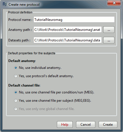
Menu File > Create new protocol > TutorialNeuromag, with the following options:
No, use individual anatomy,
No, use one channel file per run.
Import the anatomy
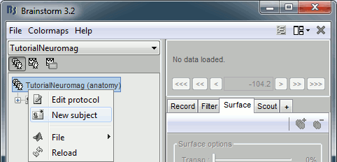
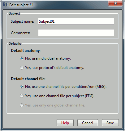
Right-click on the TutorialNeuromag folder > New subject > Subject01 (leave all the defaults).
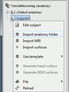
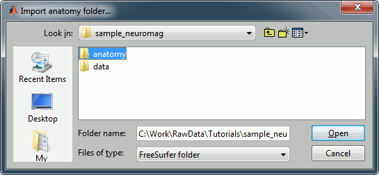
Right-click on the subject node > Import anatomy folder:
Set the file format: "FreeSurfer folder"
Select the folder: sample_neuromag/anatomy
Number of vertices of the cortex surface: 15000 (default value)
- Set the 6 required fiducial points (indicated in MRI coordinates):
- NAS: x=131, y=232, z=123
- LPA: x=48, y=136, z=74
- RPA: x=204, y=131, z=67
- AC: x=127, y=143, z=118
- PC: x=127, y=117, z=111
- IH: x=127, y=120, z=167 (anywhere on the midsagittal plane)
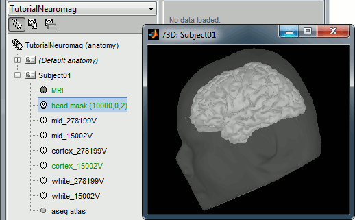
At the end of the process, make sure that the file "cortex_15000V" is selected (downsampled pial surface, that will be used for the source estimation). If it is not, double-click on it to select it as the default cortex surface.
Access the recordings
Link the FIF file to the database
- The sample_neuromag package contains one run for one subject only.
- Switch to the "functional data" view, the middle button in the toolbar above the database explorer.
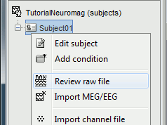
Right click on the Subject01 > Review raw file:
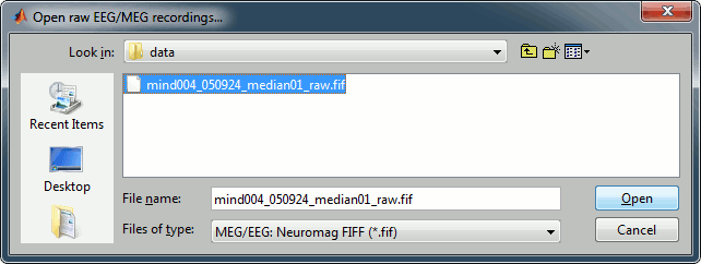
Select the file format: MEG/EEG Neuromag FIFF (*.fif)
Pick the file: sample_neuromag/data/mind004_050924_median01_raw.fif
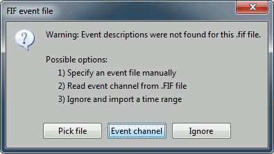
Select "Event channel" when asked about the events.
Then you have to select from which technical tracks you want to read the events.
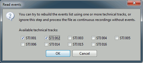
- In this dataset, the tracks of interest are:
STI 001: Contains the onsets of the electric stimulation of the right arm.
STI 002: Contains the onsets of the electric stimulation of the left arm.
- These are not standard settings, they depend on your acquisition setup. In most cases, you would rather import "events" defined with the Neuromag acquisition software, which are saved in tracks STI 014, STI 101, STI 201...
Select STI 001 and STI 002. The full tracks are read, all the changes of values are detected from these two tracks and a list of events is created.
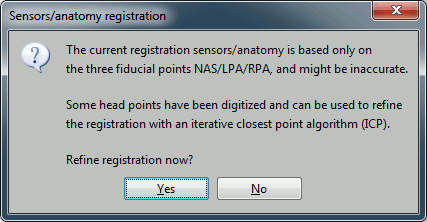
At the end, you're asked if you want to "Refine the registration with the head points". This operation improves the initial MRI/MEG registration by fitting the head points digitized at the MEG acquisition and the scalp surface. Answer YES.
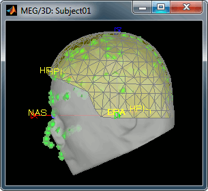
Always make sure that the final registration looks good. The yellow surface represents the inner surface of the MEG helmet and the green dots represent the head points that were saved with the MEG recordings. In this case the registration looks acceptable. If you consider it is not the case, you can fix it manually: right-click on the channel file > MRI registration > Edit.
Review the recordings
Right-click on the "Link to raw file" to see what types of channels are available:
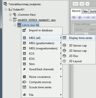
MEG (all): Represents all the MEG sensors in the file (magnetometers and gradiometers)
MEG (magnetometers): 101 magnetometers (sensor names ending with a "1")
MEG (gradiometers): 202 planar gradiometers (sensor names ending with "2" or "3")
ECG: Electro-cardiogram
EOG: Electro-oculogram
Stim: All the stimulation lines
- Double-click on the file to display all the MEG sensors.
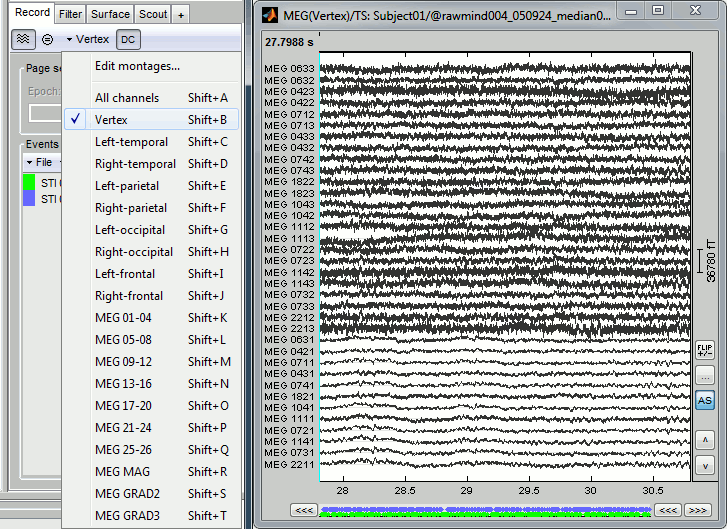
In the Record tab, look at the list of the available default display configurations for the Neuromag Vectorview MEG systems. If you would like to use different combinations of sensors, you can create your own combinations with the entry "Edit montages..."
Pre-processing
Evaluate the recordings
- Drag and drop the "Link to raw file" into the Process1 list.
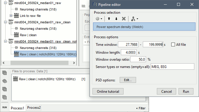
Select the process "Frequency > Power spectrum density", configure it as follows:
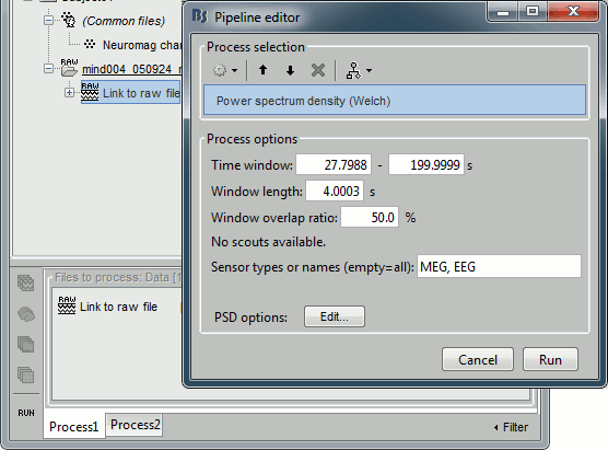
- In all the processes, the types of sensors can be specified using the following convention:
MEG: All the MEG sensors
MEG MAG: All the magnetometers
MEG GRAD: All the gradiometers
MEG GRAD2: Only the first axial gradiometer on each chip (name ends with a "2")
MEG GRAD3: Only the second axial gradiometer on each chip (name ends with a "3")
Double-click on the PSD file to display it.
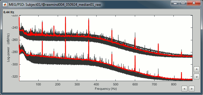
- This power spectrum shows that there is no MEG sensor that is clearly bad, but some sensors show a strong contamination from the power lines (60Hz and harmonics).
Remove: 60Hz and harmonics
Preliminary note: This process is very time and resource consuming. If you are not planning to analyze anything specifically around 60Hz, you may want to skip this section and and the long computation time associated with it. It is described here as a reference for users who would need it.
The standard procedure illustrated for removing the 60Hz power line noise illustrated in the CTF-based introduction tutorial would be simply to run the process "Pre-process > Notch filter" on the continuous file. However, this case is a bit more complicated.
If you try to run this process without selecting the option "Process the entire file at once", you would get the following error. The file already contains some SSP projectors, created by one of the Neuromag progams. Using these projectors requires all the sensors, and running frequency filters requires all the time samples at once. As a consequence, the entire file must be read in one block in order to apply frequency filters on it.
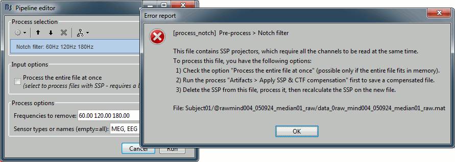
- Alternatively, if you try with the option "Process the entire file at once", you would probably crash Matlab or freeze your computer because of a lack of memory. The file is already large and this process requires to create a lot of matrices of the same size in memory. Do not try this unless you have at least 24Gb of memory available on your computer.
- The solution is to re-write an intermediate file with the SSP projectors applied, that you will be able to process easily after.
Select the "Link to raw file" in Process1 and run process "Artifacts > Apply SSP and CTF compensation". This creates a new .fif file which is an exact copy of the original .fif file, but with the SSP projectors applied to the recordings values (instead of being just saved as linear operators on the side).
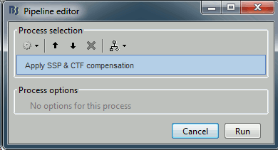
Clear the Process1 list and select the new continuous file "Raw | clean"
Run the process "Pre-process > Notch filter", configured as follows:
(this may take a while complete...)
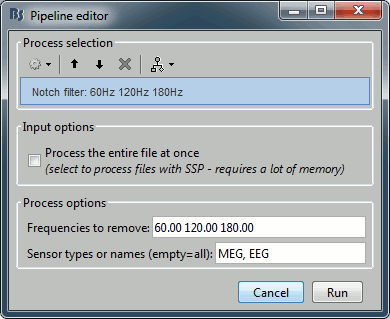
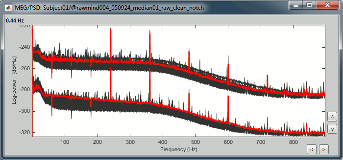
To evaluate the results of this process, select the last file generated ("Raw | clean | notch") and run again the process "Frequency > Power spectrum density".
You should observe a significant decrease of the contributions of the removed frequencies (60Hz, 120Hz, 180Hz) compared with the original spectrum.
Heartbeats and eye blinks
Signal Space Projection (SSP) is a method for projecting the recordings away from stereotyped artifacts, such as eye blinks and heartbeats.
Double-click on the last continuous file you got to display all the MEG recordings.
("Raw | clean | notch" with the notch filter, or "Link to raw file" without)Right-click on the link > ECG > Display time series, to look at the heartbeats.
Right-click on the link > EOG > Display time series, to look at the eye movements.
- From the SSP menu in the Record tab, run the automatic detections:
Detect heartbeats: Select channel ECG 063, event name "cardiac".

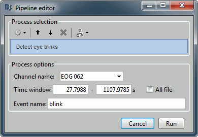
Detect eye blinks: Select channel EOG 062, event name "blink".
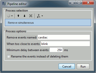
Remove simultaneous: To avoid capturing ocular artifacts in the cardiac SSP.
Remove events named: "cardiac"
When too close from events: "blink"
Minimum delay between events: 250ms.
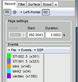
Review the traces of ECG/EOG channels and make sure the events detected make sense.
- From the same menu, run the following processes, separately for GRAD and MAG:
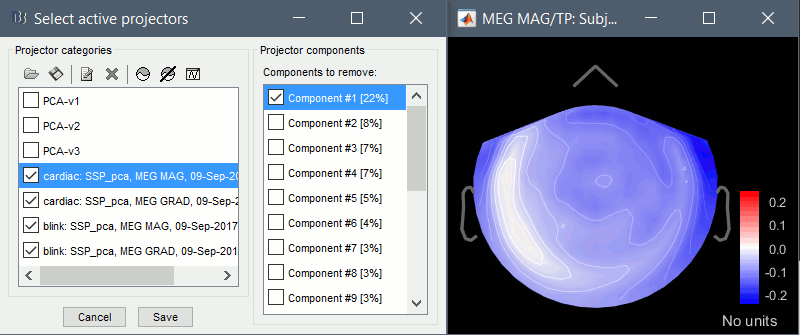
Compute SSP: Heartbeats: Event "cardiac", sensor types="MEG MAG", use existing SSP.
(select component #1)
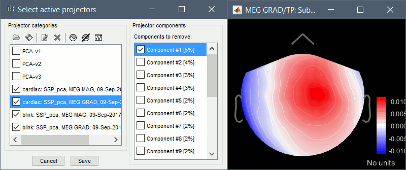
Compute SSP: Heartbeats: Event "cardiac", sensor types="MEG GRAD", use existing SSP.
(select component #1)
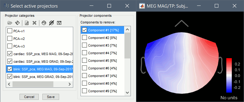
Compute SSP: Eyeblinks: Event "blink", sensor types="MEG MAG", use existing SSP.
(select component #1)
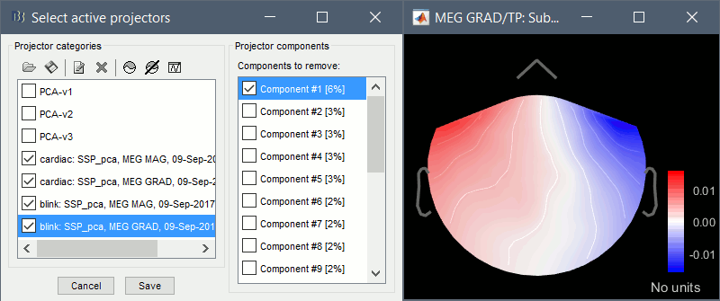
Compute SSP: Eyeblinks: Event "blink", sensor types="MEG GRAD", use existing SSP.
(select component #1)
For more information regarding this SSP method, refer to this tutorial:
?Detect and remove artifacts.At this stage, you should also review the entire file (pressing repeatedly F3) to detect any obvious bad segment in the recordings. If you detect any, select the time window to mark as bad, right click on the figure > Reject time segment.
Epoching and averaging
Import the recordings
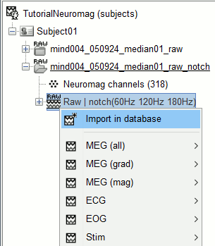
Right-click on the raw link > Import in database.
The following figure appears, that asks how to import these recordings in the Brainstorm database.
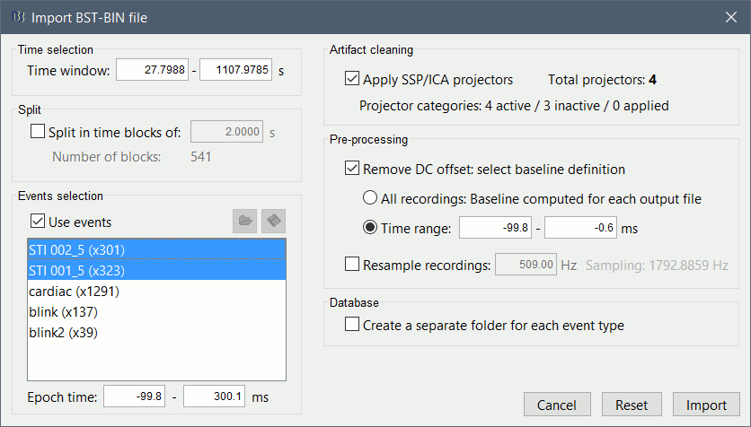
Time window: Time range of interest, keep all the time definition.
Split: Useful to import continuous recordings without events. We do not need this here.
Events selection: Check the "Use events" option, and select both STI 001 and STI 002. The values in the parenthesis represent the number of occurrences of each event.
Epoch time: Time instants that will be extracted before an after each event, to create the epochs that will be saved in the database. Set it to [-100, +300] ms
Use Signal Space Projections: Save and use the SSP vectors created by MaxFilter, MNE and Brainstorm. Keep this option selected.
Remove DC Offset: Check this option, and select: Time range: [-100, 0] ms.
For each epoch, this will: compute the average of each channel over the baseline (pre-stimulus interval: -100ms to 0ms), then subtract it from the channel at all the times in [-100,+300]ms.Resample recordings: Keep this unchecked
Create a separate folder for each epoch type: If selected, a new folder is created for each event type (here, it will create two folders "STI 001" and "STI 002"). If not selected, all the epochs from all the selected events are saved in the same folder.
- Click on [Import] and wait.
Rename the condition "STI_001_5" and "STI_002_5" into respectively "Right" and "Left" (Right-click > Rename, or press F2, or click twice waiting a while before the two clicks).
Rename the groups of trials to Left and Right.

At this stage, you should review the trials one after the other (press F3 to jump to the next file), separately for the magnetometers and the gradiometers, to make sure that you don't have any bad trial that have been imported. If you find a bad trial: right-click on the file or on the figure > Reject trial.
Averaging
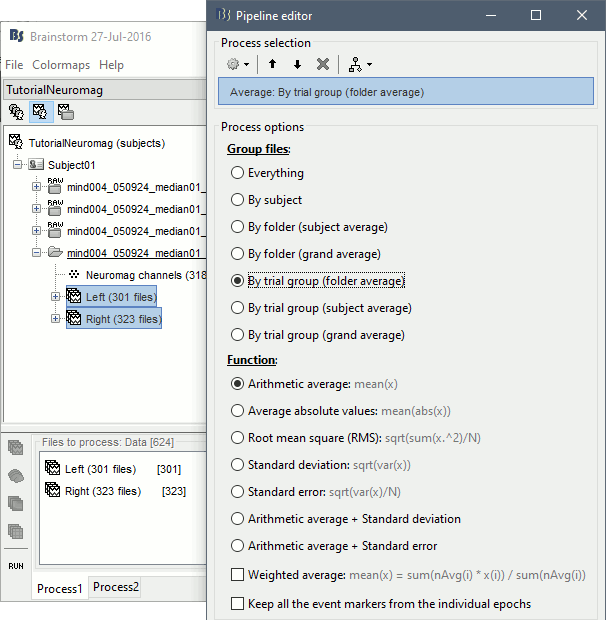
- Drag and drop all the left and right trials to the Process1 tab.
Run the process Average > Average files > By condition:
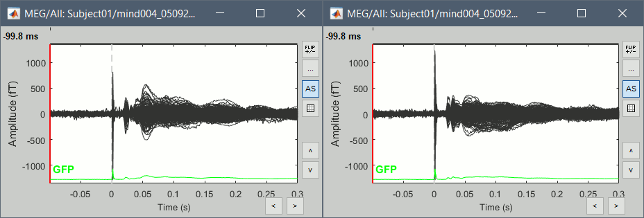
Double-click on the Left and Right averages to display all the MEG sensors:
Stimulation artifact
- We see clearly our evoked responses in these figures, but the stimulation artifact between 0ms and 4ms causes the automatic scaling of the figures to be too high, especially for the right stimulation. This effect would get a lot worse when displaying the sources for these files. To get a better display of these averages, we can cut these peaks at 0ms by replacing the values with linear interpolations.
- Select the averages for the Left and Right condition in the Process1 tab.
Run the process Artifacts > Cut stimulation artifact: 0-4ms, overwrite
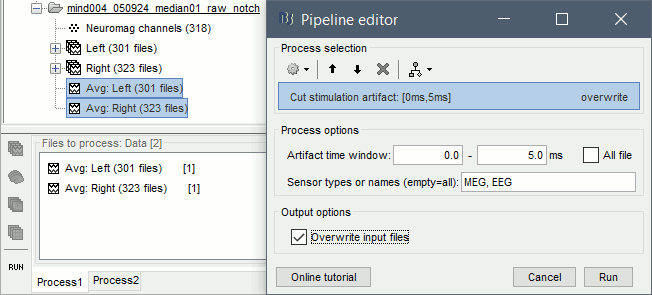
Now you can display the Left and Right averages correctly: Right-click on the file > MEG (All) > Display time series.
Display the 2D topographies for each average: Right-click on the file > MEG (All) > 2D Sensor cap (or press CTRL+T from the time series figures).
You can also add a low-pass filter at 100Hz for the visualization.
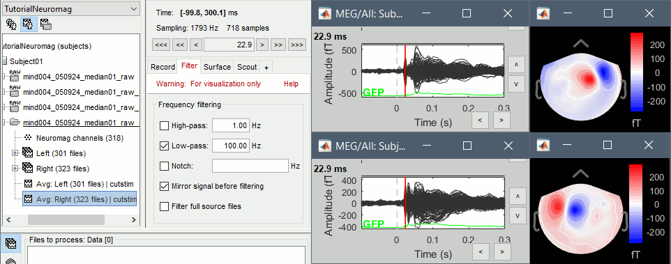
- Everything looks ok, the time series figures show a clean signal with a very high SNR, and the topographies at the first response peak (about 22ms) show an activity on the left side for the Right condition, and on the right side for the Left condition.
Gradiometers & magnetometers
Scaling factor
Magnetometers record values in Tesla (T), while gradiometers record values in Tesla per meter (T/m). The range of values obtained is not the same, therefore it is difficult to represent the two types of signals in the same figures.
We can convert the gradiometers values from T/m to T by multiplying them with the distance between the two gradiometer coils (0.0168 meters on the VectorView MEG system). But this still produces values that are too small to be represented with the same scale as the magnetometers. A more practical multiplication factor of 0.04 was proposed by Matti Hamalainen.
In the time series figure and for Elekta-Neuromag systems (all versions), the gradiometer values are always multiplied by 0.04. This is an empirical scaling factor that is used for visualization only, it is never saved in the recordings and is not used for any other purpose.
Magnetic interpolation
You can also display the MEG MAG (top) and MEG GRAD (bottom) sensors separately:
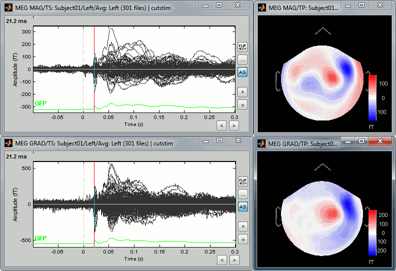
- The topographies look very similar, because all the values are re-interpolated on a surface of virtual magnetometers. To display the real values for the different types of sensors, without this magnetic interpolation, use the menus "No magnetic interpolation".
Right-click on Left > MEG (mag) > No magnetic interpolation > 2D Sensor cap.
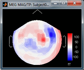
- Repeat the same operation for "MEG (gradiometers)". You now have three options, because it is not possible to display at the same time the values for the two planar gradiometers:
- Grad 2: First gradiometer, sensor names ending with "2"
- Grad 3: Second gradiometer, sensor names ending with "3"
Grad norm: Norm of the two gradiometers => sqrt(grad22 + grad32)
The three options side-by-side at 22ms (grad 2, grad3, norm):

Source estimation
We need now to calculate a source model for these recordings, using a noise covariance matrix calculated from the pre-stimulation baselines. This process is not detailed a lot here because it is very similar to what is shown in the CTF-based introduction tutorials.
Head model
Right-click on the channel file > Compute head model.
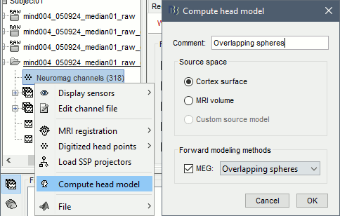
Use the overlapping spheres model and keep all of the options at their default values.
![[ATTACH] [ATTACH]](/moin_static198/brainstorm1/img/attach.png)
For more information: ?Head model tutorial.
Noise covariance
Select all the Left and Right trials, right-click > Noise covariance > Compute from recordings.
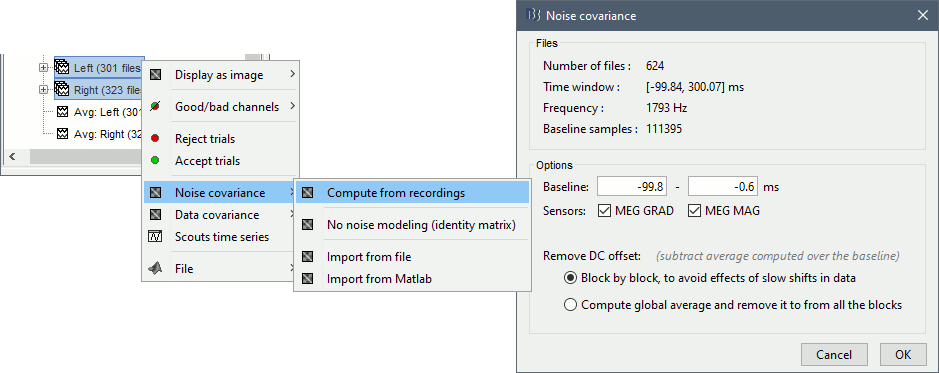
For more information: ?Noise covariance tutorial.
Inverse model
Right-click on the headmodel > Compute sources.
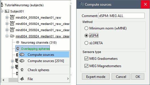
Select wMNE and all the default options. This will run a source reconstruction grouping the information from the magnetometers and the gradiometers into the same model. This is the recommended procedure, but you can also estimate sources for the two types of sensors separately if needed.
![[ATTACH] [ATTACH]](/moin_static198/brainstorm1/img/attach.png)
A shared inversion kernel is created in the (Common files) folder, and a link node is now visible for each recording file, single trials and averages.
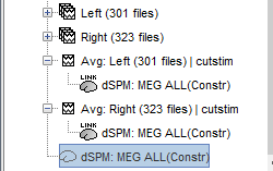
For more information: ?Source estimation tutorial.
Scouts
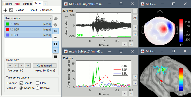
You can easily reproduce exactly the same results as the ones presented in the introduction tutorials. Place scouts to capture the activity in the primary and secondary somatosensory areas to track the processing of the electric stimulations in time, at the surface surface of the brain.
Scripting
The operations described in this tutorial can be reproduced from a Matlab script, available in the Brainstorm distribution: brainstorm3/toolbox/script/tutorial_neuromag.m
Discussion
Combining magneto+gradiometers: http://neuroimage.usc.edu/forums/showthread.php?1900
