|
Size: 24740
Comment:
|
Size: 33604
Comment:
|
| Deletions are marked like this. | Additions are marked like this. |
| Line 1: | Line 1: |
| = MEG visual tutorial: Single subject = | = MEG visual tutorial: Single subject (BIDS) = '''[WORK IN PROGRESS: THIS TUTORIAL IS NOT READY FOR PUBLIC USE]''' |
| Line 4: | Line 6: |
| The aim of this tutorial is to reproduce in the Brainstorm environment the analysis described in the SPM tutorial "[[ftp://ftp.mrc-cbu.cam.ac.uk/personal/rik.henson/wakemandg_hensonrn/Publications/SPM12_manual_chapter.pdf|Multimodal, Multisubject data fusion]]". The data processed here consists in simultaneous MEG/EEG recordings of 19 subjects performing simple visual task on a large number of famous, unfamiliar and scrambled faces. The analysis is split in two tutorial pages: the present tutorial describes the detailed analysis of one single subject and another one that describes the batch processing and [[Tutorials/VisualGroup|group analysis of the 19 subjects]]. Note that the operations used here are not detailed, the goal of this tutorial is not to teach Brainstorm to a new inexperienced user. For in depth explanations of the interface and the theory, please refer to the [[http://neuroimage.usc.edu/brainstorm/Tutorials#Get_started|introduction tutorials]]. |
The aim of this tutorial is to reproduce in the Brainstorm environment the analysis described in the SPM tutorial "[[ftp://ftp.mrc-cbu.cam.ac.uk/personal/rik.henson/wakemandg_hensonrn/Publications/SPM12_manual_chapter.pdf|Multimodal, Multisubject data fusion]]". We use here a recent update of this dataset, reformatted to follow the [[http://bids.neuroimaging.io|Brain Imaging Data Structure (BIDS)]], a standard for neuroimaging data organization. It is part of a collective effort to document and standardize MEG/EEG group analysis, see Frontier's research topic: [[https://www.frontiersin.org/research-topics/5158|From raw MEG/EEG to publication: how to perform MEG/EEG group analysis with free academic software]]. The data processed here consists of simultaneous MEG/EEG recordings from 16 participants performing a simple visual recognition task from presentations of famous, unfamiliar and scrambled faces. The analysis is split in two tutorial pages: the present tutorial describes the detailed interactive analysis of one single subject; the second tutorial describes batch processing and [[Tutorials/VisualGroup|group analysis of all 16 participants]]. Note that the operations used here are not detailed, the goal of this tutorial is not to introduce Brainstorm to new users. For in-depth explanations of the interface and theoretical foundations, please refer to the [[http://neuroimage.usc.edu/brainstorm/Tutorials#Get_started|introduction tutorials]]. |
| Line 13: | Line 15: |
| These data are provided freely for research purposes only (as part of their Award of the BioMag2010 Data Competition). If you wish to publish any of these data, please acknowledge Daniel Wakeman and Richard Henson. The best single reference is: Wakeman DG, Henson RN, [[http://www.nature.com/articles/sdata20151|A multi-subject, multi-modal human neuroimaging dataset]], Scientific Data (2015) Any questions, please contact: rik.henson@mrc-cbu.cam.ac.uk |
This dataset was obtained from the OpenfMRI project (http://www.openfmri.org), accession #ds117. It is made available under the Creative Commons Attribution 4.0 International Public License. Please cite the following reference if you use these data: Wakeman DG, Henson RN, [[http://www.nature.com/articles/sdata20151|A multi-subject, multi-modal human neuroimaging dataset]], Scientific Data (2015) Any questions regarding the data, please contact: rik.henson@mrc-cbu.cam.ac.uk |
| Line 19: | Line 21: |
| * 19 subjects (three are excluded from the group analysis for various reasons) * 6 acquisition runs (sessions) of approximately 10mins for each subject |
* 16 subjects (the original version of the dataset included 19 subjects, but 3 were excluded from the group analysis for [[http://neuroimage.usc.edu/brainstorm/Tutorials/VisualSingleOrig#Bad_subjects|various reasons]]) * 6 acquisition runs of approximately 10mins for each subject |
| Line 22: | Line 24: |
| * The subject has to judge the left-right symmetry of each stimulus * Total of nearly 300 trials in total for each of the 3 conditions |
* Participants had to judge the left-right symmetry of each stimulus * Total of nearly 300 trials for each of the 3 conditions |
| Line 31: | Line 33: |
| * MEG data have been "cleaned" using Signal-Space Separation as implemented in MaxFilter 2.2. | |
| Line 38: | Line 39: |
| * The distribution includes MEG noise recordings acquired at a similar period, processed with MaxFilter 2.2 in a way similar to the subject recordings. | * MaxFilter/tSSS: The data repository includes both the raw MEG recordings and the data cleaned using Signal-Space Separation as implemented in Elekta MaxFilter 2.2. The data was collected with continuous head localization and cannot be processed easily without running the algorithms SSS or tSSS. Brainstorm currently does not offer any free alternative to MaxFilter, therefore in this tutorial we will import the recordings already processed with MaxFilter's tSSS, available in the "derivatives" folder of the BIDS architecture. To save disk space, will not download the raw MEG recordings. This means we will not get any of the additional files available in the BIDS structure (headshape, events, channels) but it doesn't matter because all the information is directly available in the .fif files. * The data distribution includes MEG noise recordings acquired around the dates of the experiment, processed with MaxFilter 2.2 in the same way as the experimental data. |
| Line 41: | Line 43: |
| * MRI data acquired on a 3T Siemens TIM Trio: 1x1x1mm T1-weighted structural MRI * Processed with FreeSurfer 5.3 |
* MRI data acquired on a 3T Siemens TIM Trio: 1x1x1mm T1-weighted structural MRI. * The face was removed from the structural images for anonymization purposes. * Processed with FreeSurfer 5.3. |
| Line 45: | Line 48: |
| * The data is hosted on the OpenfMRI website: https://openfmri.org/dataset/ds000117/ * Download all the files available for dowload from this website (approximately 160Gb):<<BR>>ds117_metadata.tgz, ds117_sub001_raw.tgz, ..., ds117_sub019_raw.tgz * Unzip all the .tgz files in the same folder. * The FreeSurfer segmentations of the T1 images are not part of this package. You can either process them by yourself, or download the result of the segmentation from the Brainstorm website. <<BR>>Go to the [[http://neuroimage.usc.edu/bst/download.php|Download]] page, and download the file: '''sample_group_freesurfer.zip'''<<BR>>Unzip this file in the same folder where you downloaded all the datasets. * We will use the following files from this distribution: * '''/anatomy/subXXX/''': Segmentation folders generated with FreeSurfer. * '''/emptyroom/090707_raw_st.fif''': MEG empty room measurements, processed with MaxFilter. * '''/ds117/subXXX/MEG/*_sss.fif''': MEG and EEG recordings, processed with MaxFilter. * '''/README''': License and dataset description. * Reminder: Do not put the downloaded files in the Brainstorm folders (program or database folders). |
* First, make sure you have enough space on your hard drive, at least '''400Gb''': * Raw files: '''170Gb''' * Processed files: '''230Gb''' * Download the entire dataset from the OpenNeuro website (one single .tar file): <<BR>>[[https://openfmri.org/dataset/ds000117/|https://openneuro.org/datasets/ds000117/versions/00004]] <<BR>><<BR>> {{attachment:ds000117_download.gif||width="592",height="232"}} * Expand the .tar files in the same folder: * Linux/MacOS: Run "tar -vf filename.tar" from a terminal * Windows: Install a free utility (eg. 7zip, WinRAR), right-click on the file.tar > Extract * '''Reminder''': Do not save the downloaded files in the Brainstorm program or database folders * In this tutorial, we will use only the derivatives folder (85Gb), if you need to make some space on your hard drive you can delete all the other folders. Files we will use here: * FreeSurfer anatomy: /derivatives/freesurfer/sub-XX/ses-mri/anat/* * MEG recordings (SSS): /derivatives/meg_derivatives/sub-XX/ses-meg/meg/*.fif * Empty-room (SSS): /derivatives/meg_derivatives/sub-emptyroom/ses-meg/meg/*.fif |
| Line 62: | Line 73: |
| This page explains how to import and process subject '''#002''' only. Subject #001 will be later excluded from the EEG group analysis because the position of the electrodes is incorrect, so it was not the best example. | This dataset is formatted following the [[https://www.biorxiv.org/content/early/2017/08/08/172684|BIDS-MEG specifications]], therefore we could import all the [[http://neuroimage.usc.edu/brainstorm/Tutorials/LabelFreeSurfer|relevant information]] (MRI, FreeSurfer segmentation, MEG+EEG recordings) in just one click, with the menu '''File > Load protocol''' > '''Import BIDS dataset''', as described in the online tutorial [[http://neuroimage.usc.edu/brainstorm/Tutorials/RestingOmega#BIDS_specifications|MEG resting state & OMEGA database]]. However, because your own data might not be organized following the BIDS standards, in this tutorial we preferred illustrating all the detailed steps for importing the data rather than the BIDS shortcut. Plus, we will need some additional steps that are not part of the standard import, because of the data anonymization (MRI were defaced and acquisition dates removed). This page explains how to import and process the first run of '''subject''' '''#01''' only. All the other files will have to be processed in the same way. |
| Line 65: | Line 78: |
| * Right-click on the TutorialAuditory folder > New subject > '''sub002''' * Leave the default options you set for the protocol * Right-click on the subject node > Import anatomy folder: |
* Right-click on the TutorialVisual folder > New subject > '''sub-01''' * Leave the default options you defined for the protocol. * Right-click on the subject node > '''Import anatomy folder''': |
| Line 69: | Line 82: |
| * Select the folder: '''anatomy/freesurfer/sub002''' (from sample_group_freesurfer.zip) | * Select the folder: '''derivatives/freesurfer/sub-01/ses-mri/anat''' |
| Line 71: | Line 84: |
| * The two sets of fiducials we usually have to define interactively are here automatically set. * '''NAS/LPA/RPA''': The file Anatomy/Sub01/fiducials.m contains the definition of the nasion, left and right ears. The anatomical points used by the authors are the same as the ones we recommend in the Brainstorm [[CoordinateSystems|coordinates systems page]]. * '''AC/PC/IH''': Automatically identified using the SPM affine registration with an MNI template. * If you want to double-check that all these points were correctly marked after importing the anatomy, right-click on the MRI > Edit MRI. * At the end of the process, make sure that the file "cortex_15000V" is selected (downsampled pial surface, that will be used for the source estimation). If it is not, double-click on it to select it as the default cortex surface. Do not worry about the big holes in the head surface, parts of MRI have been remove voluntarily for anonymization purposes.<<BR>><<BR>> {{attachment:anatomy_import.gif||height="384",width="613"}} * All the anatomical atlases [[Tutorials/LabelFreeSurfer|generated by FreeSurfer]] were automatically imported: the surface-based cortical atlases and the atlas of sub-cortical regions (ASEG). <<BR>><<BR>> {{attachment:anatomy_atlas.gif||height="211",width="550"}} |
* When asked to select the anatomical fiducials, click on "'''Compute MNI transformation'''". This will register the MRI volume to an [[http://neuroimage.usc.edu/brainstorm/CoordinateSystems#MNI_coordinates|MNI template]] with an affine transformation, using SPM functions embedded in Brainstorm (spm_maff8.m). This will also place default fiducial points NAS/LPA/RPA in the MRI, based on MNI coordinates. We will use digitized head points for the [[https://neuroimage.usc.edu/brainstorm/Tutorials/ChannelFile#Automatic_registration|MEG-MRI coregistration]], therefore we don't need accurate anatomical positions here. * Note that if you don't have a good digitized head shape for the subject, or if the final registration MEG-MRI doesn't look good with this head shape, you should not skip this step and mark accurate NAS/LPA/RPA fiducial points in the MRI, using the same anatomical convention that was used during the MRI acquisition. * Then click on [Save] to start the import. * At the end of the process, make sure that the file "cortex_15000V" is selected (downsampled pial surface, that will be used for the source estimation). Otherwise, double-click on it to select it as the default cortex surface. Do not worry about the big holes in the head surface, parts of MRI have been remove voluntarily for anonymization purposes.<<BR>><<BR>> {{attachment:anatomy_import.gif||width="613",height="384"}} * All the anatomical atlases [[Tutorials/LabelFreeSurfer|generated by FreeSurfer]] were automatically imported: the cortical atlases (Desikan-Killiany, Mindboggle, Destrieux, Brodmann) and the sub-cortical regions (ASEG atlas). <<BR>><<BR>> {{attachment:anatomy_atlas.gif||width="550",height="211"}} |
| Line 87: | Line 99: |
| * Select the '''first''' FIF files in: '''Sub001/MEEG''' <<BR>><<BR>> {{attachment:review_raw.gif||height="202",width="542"}} * Events:''' Ignore'''<<BR>>We will read events for the stimulus channel and define trial definitions later.<<BR>><<BR>> {{attachment:review_ignore.gif||height="186",width="330"}} |
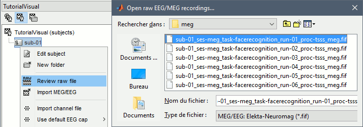
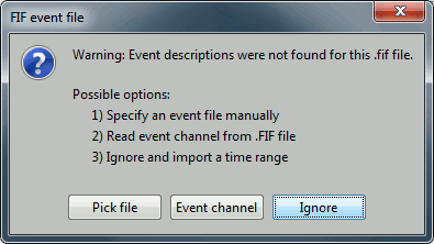
* Go to the folder: '''derivatives/meg_derivatives/sub-01/ses-meg/meg''' * Select file: '''sub-01_ses-meg_task-facerecognition_run-01_proc-sss_meg.fif''' <<BR>><<BR>> {{attachment:review_raw.gif||width="583",height="205"}} * Events:''' Ignore'''. We will read the stimulus triggers later.<<BR>><<BR>> {{attachment:review_ignore.gif||width="330",height="186"}} |
| Line 97: | Line 110: |
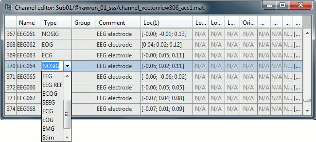
| * Change the type of '''EEG061''' and '''EEG064''' to '''NOSIG'''. Close the window and save the modifications. <<BR>><<BR>> {{attachment:channel_edit.gif||height="252",width="561"}} | * Change the type of '''EEG061''' and '''EEG064''' to '''NOSIG''' (or any other non-informative type). Close the window and save the modifications. <<BR>><<BR>> {{attachment:channel_edit.gif||width="561",height="252"}} |
| Line 100: | Line 113: |
| At this point, the registration MEG/MRI is based only the three fiducial points NAS/LPA/RPA. All the anatomical scans were anonymized (defaced) and for some subjects the nasion could not be defined properly. We will try to refine this registration using the additional head points that were digitized (only the points above the nasion). * Right-click on the channel file > '''Digitized head points > Remove points below nasion'''.<<BR>><<BR>> {{attachment:channel_remove.gif||height="194",width="329"}} * Right-click on the channel file > '''MRI registration > Refine using head points'''.<<BR>><<BR>> {{attachment:channel_refine.gif||height="173",width="294"}} * MEG/MRI registration, before (left) and after (right) this automatic registration procedure: <<BR>><<BR>> {{attachment:registration.gif||height="209",width="236"}} {{attachment:registration_final.gif||height="208",width="237"}} * Right-click on the channel file > MRI registration > EEG: Edit...<<BR>>Click on ['''Project electrodes on surface''']<<BR>><<BR>> {{attachment:channel_project.gif||height="207",width="477"}} * Close all the windows (use the [X] button at the top-right corner of the Brainstorm window). === Import event markers === We need to read the stimulus markers from the STI channels. The following tasks can be done in an interactive way with menus in the Record tab, as in the introduction tutorials. We will here illustrate how to do this with the pipeline editor, it will be easier to batch it for all the runs and all the subjects. |
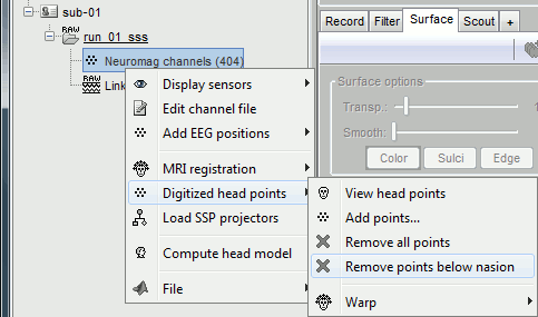
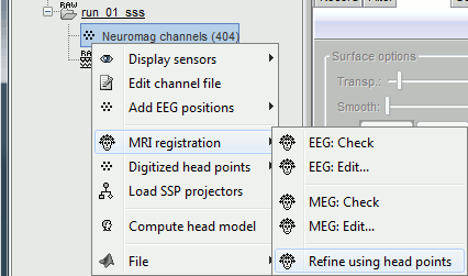
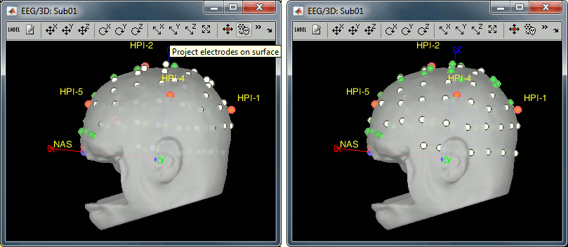
At this point, the registration MEG/MRI is based only on the three anatomical landmarks NAS/LPA/RPA, which are not even accurately set (we used default MNI positions). All the MRI scans were anonymized (defaced) so all the head points below the nasion cannot be used. We will try to refine this registration using the additional head points that were digitized above the nasion. * Right-click on the channel file > '''Digitized head points > Remove points below nasion'''. <<BR>>(42 points removed, 95 head points left)<<BR>><<BR>> {{attachment:channel_remove.gif||width="329",height="194"}} * Right-click on the channel file > '''MRI registration > Refine using head points'''.<<BR>><<BR>> {{attachment:channel_refine.gif||width="294",height="173"}} * MEG/MRI registration, before (left) and after (right) this automatic registration procedure: <<BR>><<BR>> {{attachment:registration.gif||width="236",height="209"}} {{attachment:registration_final.gif||width="237",height="208"}} * Right-click on the channel file > '''MRI registration > EEG: Edit'''.<<BR>>Click on ['''Project electrodes on surface'''], then close the figure to save the modifications.<<BR>><<BR>> {{attachment:channel_project.gif||width="477",height="207"}} === Read stimulus triggers === We need to read the stimulus markers from the STI channels. The following tasks can be done in an interactive way with menus in the Record tab, as in the introduction tutorials. We will illustrate here how to do this with the pipeline editor, it will be easier to batch it for all the runs and all the subjects. |
| Line 112: | Line 124: |
| * Select process '''Events > Read from channel''', Channel: '''STI101''', Detection mode: '''Bit'''.<<BR>>Do not execute the process, we will add other processes to classify the markers.<<BR>><<BR>> {{attachment:raw_read_events.gif||height="290",width="499"}} * We want to create three categories of events: * Famous faces: 5 (00101), 6 (00110), 7 (00111) => Bit 3 only * Unfamiliar faces: 13 (01101), 14 (01110), 15 (01111) => Bit 3 and 4 * Scrambled images: 17 (10001), 18 (10010), 19 (10011) => Bit 5 only * We will start by creating the category "Unfamiliar" (combination of events "3" and "4") and remove the remove the initial events. Then we just have to rename the renaming "3" in "Famous", and all the "5" in "Scrambled". |
* Select process '''Events > Read from channel''', Channel: '''STI101''', Detection mode: '''Bit'''.<<BR>>Do not execute the process, we will add other processes to classify the markers.<<BR>><<BR>> {{attachment:raw_read_events.gif||width="499",height="290"}} * We want to create three categories of events, based on their numerical codes: * '''Famous faces''': 5 (00101), 6 (00110), 7 (00111) => Bit 3 only * '''Unfamiliar faces''': 13 (01101), 14 (01110), 15 (01111) => Bit 3 and 4 * '''Scrambled images''': 17 (10001), 18 (10010), 19 (10011) => Bit 5 only * We will start by creating the category "Unfamiliar" (combination of events "3" and "4") and remove the remove the initial events. Then we just have to rename the remaining "3" in "Famous", and all the "5" in "Scrambled". |
| Line 121: | Line 133: |
| * Add process '''Events > Rename event''': 5 => Scrambled <<BR>><<BR>> {{attachment:events_merge.gif||height="402",width="532"}} * Add process '''Events > Add time offset''' to correct for the presentation delays:<<BR>>Event names: "'''Famous, Unfamiliar, Scrambled'''", Time offset = '''34.5ms'''<<BR>><<BR>> {{attachment:events_offset.gif||height="355",width="348"}} * Finally run the script. Double-click on the recordings to make sure the labels were detected correctly. You can delete the unwanted events that are left in the recordings (1,2,9,13): <<BR>><<BR>> {{attachment:events_display.gif||height="194",width="595"}} |
* Add process '''Events > Rename event''': 5 => Scrambled <<BR>><<BR>> {{attachment:events_merge.gif||width="532",height="402"}} * Add process '''Events > Add time offset''' to correct for the presentation delays:<<BR>>Event names: "'''Famous, Unfamiliar, Scrambled'''", Time offset = '''34.5ms'''<<BR>><<BR>> {{attachment:events_offset.gif||width="348",height="355"}} * Finally run the script. Double-click on the recordings to make sure the labels were detected correctly. You can delete the unwanted events that are left in the recordings (1,2,9,13). Edit the colors if you don't like the default ones.<<BR>><<BR>> {{attachment:events_display.gif||width="595",height="194"}} |
| Line 129: | Line 141: |
| * Run process '''Frequency > Power spectrum density (Welch)''' with the options illustrated below. <<BR>><<BR>> {{attachment:psd_process.gif||height="314",width="669"}} * Right-click on the PSD file > Power spectrum. <<BR>><<BR>> {{attachment:psd_plot.gif||height="315",width="546"}} |
* Run process '''Frequency > Power spectrum density (Welch)''' with the options illustrated below. <<BR>><<BR>> {{attachment:psd_process.gif||width="669",height="314"}} * Right-click on the PSD file > Power spectrum. <<BR>><<BR>> {{attachment:psd_plot.gif||width="408",height="235"}} * The MEG sensors look awful, because of one small segment of data located around 248s. Open the MEG recordings and scroll to 248s (just before the first Unfamiliar event). <<BR>><<BR>> {{attachment:psd_error.gif||width="527",height="183"}} * In these recordings, the continuous head tracking was activated, but it starts only at the time of the stimulation (248s) while the acquisition of the data starts 22s before (226s). The first 22s do not have head localization coils (HPI) coils activity and are not corrected by MaxFilter. After 248s, the HPI coils are on, and MaxFilter filters them out. The transition between the two states is not smooth and creates important distortions in the spectral domain. For a proper evaluation of the recordings, we should '''compute the PSD only after the HPI coils are turned on'''. * Run process '''Events > Detect cHPI activity (Elekta)'''. This detects the changes in the cHPI activity from channel STI201 and marks all the data without head localization as bad. <<BR>><<BR>> {{attachment:psd_badsegment.gif||width="503",height="234"}} * Re-run the process '''Frequency > Power spectrum density (Welch)'''. All the bad segments are excluded from the computation, therefore the PSD is now estimated only with the data '''after 248s'''. <<BR>><<BR>> {{attachment:psd_fix.gif||width="668",height="283"}} |
| Line 135: | Line 151: |
| * Artifacts due to Elekta electronics: '''293'''Hz, '''307'''Hz, '''314'''Hz, '''321'''Hz, '''328'''Hz. | * Artifacts due to Elekta electronics (HPI coils): '''293'''Hz, '''307'''Hz, '''314'''Hz, '''321'''Hz, '''328'''Hz. * Peak from unknown source at '''103.4Hz''' in the MEG only. |
| Line 141: | Line 158: |
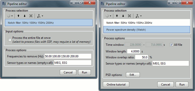
| * Select process '''Pre-process > Notch filter''' to remove the line noise (50-200Hz).<<BR>>Add immediately after the process "'''Frequency > Power spectrum density (Welch)'''" <<BR>><<BR>> {{attachment:notch_process.gif||height="262",width="562"}} * Double-click on the PSD for the new continuous file to evaluate the quality of the correction. <<BR>><<BR>> {{attachment:notch_result.gif||height="215",width="566"}} |
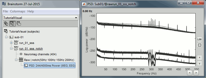
* Select process '''Pre-process > Notch filter''' to remove the line noise (50-200Hz).<<BR>>Add the process '''Frequency > Power spectrum density (Welch)'''. <<BR>><<BR>> {{attachment:notch_process.gif||width="562",height="262"}} * Double-click on the PSD for the new continuous file to evaluate the quality of the correction. <<BR>><<BR>> {{attachment:notch_result.gif||width="566",height="215"}} |
| Line 147: | Line 164: |
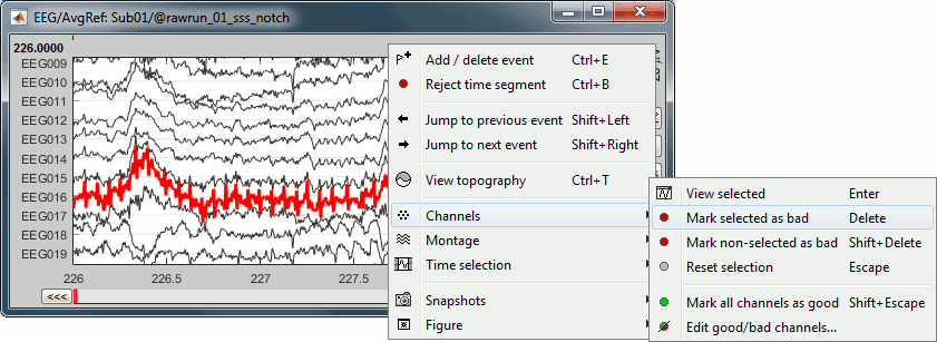
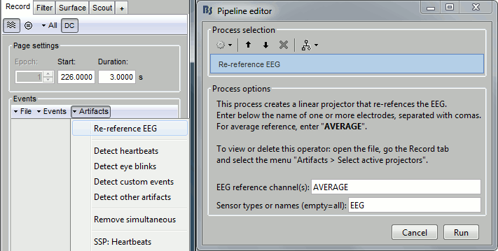
| * Select channel '''EEG016''' and mark it as '''bad''' (using the popup menu or pressing the Delete key). <<BR>><<BR>> {{attachment:channel_bad.gif||height="214",width="587"}} * In the Record tab, menu '''Artifacts > Re-reference EEG''' > "AVERAGE". <<BR>><<BR>> {{attachment:channel_ref.gif||height="270",width="535"}} |
* Select channel '''EEG016''' and mark it as '''bad''' (using the popup menu or pressing the Delete key). <<BR>><<BR>> {{attachment:channel_bad.gif||width="587",height="214"}} * In the Record tab, menu '''Artifacts > Re-reference EEG''' > "AVERAGE". <<BR>><<BR>> {{attachment:channel_ref.gif||width="535",height="270"}} |
| Line 151: | Line 168: |
| == Artifact correction with SSP == === Artifact detection === |
== Artifact detection == === Heartbeats: Detection === |
| Line 155: | Line 172: |
| * Run process''' Events > Detect heartbeats''': Channel name='''EEG063''', All file, Event name=cardiac <<BR>><<BR>> {{attachment:detect_cardiac.gif||height="230",width="310"}} * In many of the other tutorials, you will have detected the blink category and used the SSP process to remove the blink artifact. In this experiment, we are particularly interested in the subject's response to seeing the stimulus. Therefore we will mark blinks and other eye movements as BAD. * Run process '''Artifacts > Detect events above threshold''': Event name='''blink_BAD''', Channel='''EEG062''', All file, Maximum threshold='''100''', Threshold units='''uV''', Filter='''[0.30,20.00]Hz''', '''Use absolute value of signal'''.<<BR>><<BR>> {{attachment:detect_blinks.gif||height="455",width="285"}} * Inspect visually the two new cateogries: cardiac and blink_BAD.<<BR>><<BR>> {{attachment:detect_display.gif||height="237",width="655"}} |
* Run process''' Events > Detect heartbeats''': Channel name='''EEG063''', All file, Event name=cardiac <<BR>><<BR>> {{attachment:detect_cardiac.gif||width="310",height="230"}} === Eye blinks: Detection === * In many of the other tutorials, we detect the blinks and remove them with SSP. In this experiment, we are particularly interested in the subject's response to seeing the stimulus. Therefore we will exclude from the analysis all the recordings contaminated with blinks or other eye movements. * Run process '''Events > Detect events above threshold''': <<BR>>Event name='''blink_BAD''', Channel='''EEG062''', All file, Maximum threshold='''100''', Threshold units='''uV''', Filter='''[0.30,20.00]Hz''', '''Use absolute value of signal'''.<<BR>><<BR>> {{attachment:detect_blinks.gif||width="285",height="455"}} * In other tutorials, we used the process "Detect eye blinks" which creates simple events indicating the peak of the EOG signal during a blink. In this study, we preferred using this process "Detect events above threshold" because it creates extended events marking as bad all the segment for which the EOG value is above a given threshold. It's more manual but it ensures we really exclude all the ocular activity. * Inspect visually the two new cateogries of events: cardiac and blink_BAD.<<BR>><<BR>> {{attachment:detect_display.gif||width="655",height="237"}} |
| Line 165: | Line 185: |
| === Heartbeats === | === Heartbeats: Correction with SSP === |
| Line 168: | Line 188: |
| * Add process '''Artifacts > SSP: Heartbeats''' > Sensor type: '''MEG GRAD''' - Run the execution <<BR>><<BR>> {{attachment:ssp_ecg_process.gif||height="225",width="293"}} | * Add process '''Artifacts > SSP: Heartbeats''' > Sensor type: '''MEG GRAD''' - Run the execution <<BR>><<BR>> {{attachment:ssp_ecg_process.gif||width="293",height="225"}} |
| Line 172: | Line 192: |
| * In category '''cardiac/MEG GRAD''': Select '''component #1 '''and view topography. <<BR>><<BR>> {{attachment:ssp_ecg_topo.gif||height="175",width="604"}} | * In category '''cardiac/MEG GRAD''': Select '''component #1 '''and view topography. <<BR>><<BR>> {{attachment:ssp_ecg_topo.gif||width="604",height="175"}} |
| Line 177: | Line 197: |
| * Process1>Run: Select the process "'''Events > Detect other artifacts'''". This should be done separately for MEG and EEG to avoid confusion about which sensors are involved in the artifact. <<BR>><<BR>> {{attachment:detect_other.gif||height="253",width="486"}} * Display the MEG sensors. Review the segments that were tagged as artifact, determine if each event represents an artifact and then mark the time of the artifact as BAD. This can be done by selecting the time window around the artifact, Right-click > '''Reject time segment'''. Note that this detection process marks 1-second segments but the artifact can be shorter.<<BR>><<BR>> {{attachment:artifacts_mark_bad.png||width="640"}} |
* Process1>Run: Select the process "'''Events > Detect other artifacts'''". This should be done separately for MEG and EEG to avoid confusion about which sensors are involved in the artifact. <<BR>><<BR>> {{attachment:detect_other.gif||width="486",height="253"}} * Display the MEG sensors. Review the segments that were tagged as artifact, determine if each event represents an artifact and then mark the time of the artifact as BAD. This can be done by selecting the time window around the artifact, then right-click > '''Reject time segment'''. Note that this detection process marks 1-second segments but the artifact can be shorter.<<BR>><<BR>> {{attachment:artifacts_mark_bad.png||width="640"}} |
| Line 184: | Line 204: |
| MEG signals recorded with Elekta-Neuromag systems frequently contain SQUID jumps ([[http://neuroimage.usc.edu/brainstorm/Tutorials/BadSegments?highlight=(squid)#Elekta-Neuromag_SQUID_jumps|more information]]). These sharp steps followed by a change of baseline value are usually easy to identify visually but more complicated to detect automatically. The process "Detect other artifacts" usually detects most of them in the category "1-7Hz". If you observe that some are skipped, you can try re-running it with a high sensitivity. It is important to review all the sensors and all the time in each recording to be sure these events are marked as bad segments. . {{attachment:detect_jumps.gif||height="214",width="547"}} |
MEG signals recorded with Elekta-Neuromag systems frequently contain SQUID jumps ([[http://neuroimage.usc.edu/brainstorm/Tutorials/BadSegments?highlight=(squid)#Elekta-Neuromag_SQUID_jumps|more information]]). These sharp steps followed by a change of baseline value are easy to identify visually but more complicated to detect automatically. The process "Detect other artifacts" usually detects most of them in the category "1-7Hz". If you observe that some are skipped, you can try re-running it with a higher sensitivity. It is important to review all the sensors and all the time in each run to be sure these events are marked as bad segments. . {{attachment:detect_jumps.gif||width="547",height="214"}} |
| Line 194: | Line 214: |
| * Select process: '''Import recordings > Import MEG/EEG: Events''' (do not run immediately)<<BR>>Event names "Famous, Unfamiliar, Scrambled", All file, Epoch time=[-300,1000]ms * Add process: '''Pre-process > Remove DC offset''': Baseline=[-300,-0.9]ms - Run execution.<<BR>><<BR>> {{attachment:import_epochs.gif||height="399",width="647"}} === Average === |
* Select process: '''Import > Import recordings > Import MEG/EEG: Events''' (do not run immediately)<<BR>>Event names "Famous, Unfamiliar, Scrambled", All file, Epoch time=[-500,1200]ms * Add process: '''Pre-process > Remove DC offset''': Baseline=[-500,-0.9]ms - Run execution.<<BR>><<BR>> {{attachment:import_epochs.gif||width="647",height="399"}} === Average by run === |
| Line 199: | Line 219: |
| * Run process: '''Average > Average files''': '''By trial groups (folder average)''' <<BR>><<BR>> {{attachment:average_process.gif||height="504",width="478"}} | * Run process: '''Average > Average files''': '''By trial groups (folder average)''' <<BR>><<BR>> {{attachment:average_process.gif||width="478",height="504"}} |
| Line 202: | Line 222: |
| * EEG evoked response (famous, scrambled, unfamiliar): <<BR>><<BR>> {{attachment:average_topo.gif||height="392",width="684"}} * Open the [[Tutorials/ChannelClusters|Cluster tab]] and create a cluster with the channel '''EEG065''' (button [NEW IND]).<<BR>><<BR>> {{attachment:cluster_create.gif||height="166",width="569"}} * Select the cluster then select three average files, right-click > '''Clusters time series''' (Overlay:Files). <<BR>><<BR>> {{attachment:cluster_display.gif||height="220",width="658"}} |
* EEG evoked response (famous, scrambled, unfamiliar), low-pass filter at 32Hz: <<BR>><<BR>> {{attachment:average_topo.gif||width="684",height="392"}} * Open the [[Tutorials/ChannelClusters|Cluster tab]] and create a cluster with the channel '''EEG065''' (button [NEW IND]).<<BR>><<BR>> {{attachment:cluster_create.gif||width="569",height="166"}} * Select the cluster, select the three average files, right-click > '''Clusters time series''' (Overlay:Files). <<BR>><<BR>> {{attachment:cluster_display.gif||width="658",height="220"}} |
| Line 209: | Line 229: |
| == Noise covariance == The minimum norm model we will use next to estimate the source activity can be improved by modeling the the noise contaminating the data. The section shows how to [[Tutorials/NoiseCovariance|estimate the noise covariance]] in different ways for EEG and MEG. For the MEG recordings we will use the empty room measurements we have, and for the EEG we will compute it from the pre-stimulus baselines we have in all the imported epochs. === MEG: Empty room recordings === * Create a new subject: '''emptyroom''' * Right-click on the new subject > '''Review raw file'''.<<BR>>Select file: '''sample_group/emptyroom/090707_raw_st.fif '''<<BR>>Do not apply default transformation, Ignore event channel.<<BR>><<BR>> {{attachment:noise_review.gif||height="164",width="506"}} * Select this new file in Process1 and run process '''Pre-process > Notch filter''': '''50 100 150 200Hz'''. When using empty room measurements to compute the noise covariance, they must be processed exactly in the same way as the other recordings. <<BR>><<BR>> {{attachment:noise_notch.gif||height="225",width="436"}} * Right-click on the filtered noise recordings > '''Noise covariance > Compute from recordings''': <<BR>><<BR>> {{attachment:noise_compute.gif||height="240",width="649"}} * Right-click on the '''Noise covariance > Copy to other subjects '''<<BR>><<BR>> {{attachment:noise_copy.gif||height="126",width="273"}} === EEG: Pre-stimulus baseline === * In folder sub002/run_01_sss_notch, select all the imported the imported trials, right-click > '''Noise covariance > Compute from recordings''', Time=[-300,0]ms, '''EEG only''', '''Merge'''. {{attachment:noise_eeg.gif||height="280",width="650"}} * This computes the noise covariance only for EEG, and combines it with the existing MEG information. {{attachment:noise_display.gif||height="223",width="375"}} == Source estimation == |
== Source estimation [TODO] == === MEG noise covariance: Empty room recordings [TODO] === The minimum norm model we will use next to estimate the source activity can be improved by modeling the the noise contaminating the data. The introduction tutorials explain how to [[Tutorials/NoiseCovariance|estimate the noise covariance]] in different ways for EEG and MEG. For the MEG recordings we will use the empty room measurements we have, and for the EEG we will compute it from the pre-stimulus baselines we have in all the imported epochs. There are 8 empty room files available in this dataset. For each subject, we will use only one file, the one that was acquired at the closest date. We will now import and process all the empty room recordings simultaneously, even if only one is needed by the current subject. Later, for each subject we will select the most appropriate noise covariance matrix. * Create a new subject: '''sub-emptyroom''' * Right-click on the new subject > '''Review raw file'''.<<BR>>Select all the folders in: '''derivatives/sub-emptyroom '''(processed with MaxFilter/tSSS)<<BR>>Do not apply default transformation, Ignore event channel.<<BR>><<BR>> {{attachment:noise_review.gif||width="516",height="180"}} * Select all these new files in Process1 and run process '''Pre-process > Notch filter''': '''50 100 150 200Hz'''. When using empty room measurements to compute the noise covariance, they must be processed exactly in the same way as the other recordings (same MaxFilter parameters, same frequency filters). <<BR>><<BR>> {{attachment:noise_notch.gif||width="634",height="242"}} * Delete all the original noise files and keep only the filtered ones. * Identify the noise file that was recorded the closest to the subject's recordings. You can read the acquisition date of a file in the tooptip that is displayed when you leave you mouse for a while over its folder. The MEG for subject sub-01 was recorded on April 9th 2009, so we will compute the MEG noise covariance for this subject from the first noise file available, which was acquired on the same date. <<BR>><<BR>> {{attachment:noise_closest.gif}} * Right-click on the noise recordings 2009-04-09 > '''Noise covariance > Compute from recordings''': <<BR>><<BR>> {{attachment:noise_compute.gif||width="641",height="276"}} * Finally copy the noise covariance from sub-emptyroom to the folder with imported epochs in sub-01. Use the popup menus File>Copy/Paste, or the keyboard shortcuts Ctrl+C/Ctrl+V.<<BR>><<BR>> {{attachment:noise_copy.gif||width="685",height="246"}} === EEG noise covariance: Pre-stimulus baseline === * In folder sub-01/run-01_tsss_notch, select all the imported the imported trials, right-click > '''Noise covariance > Compute from recordings''', Time=[-500,-0.9]ms, '''EEG only''', '''Merge'''. {{attachment:noise_eeg.gif||width="650",height="280"}} * This computes the noise covariance only for EEG, and combines it with the existing MEG information. {{attachment:noise_display.gif||width="375",height="223"}} * To generate the corresponding analysis script, we will use a different strategy, which will match automatically the subject with the appropriate MEG noise covariance. We will first import all the subjects, compute the EEG noise covariance for all the runs, then compute the MEG noise covariance matrix for all the empty room files at once with the process "Sources > Compute covariance" with the options "Match noise and subject recordings by acquisition date", "Sensor types=MEG", "Merge". <<BR>><<BR>> {{attachment:noise_automatch.gif||width="491",height="427"}} |
| Line 225: | Line 249: |
| We will need to compute a [[Tutorials/TutBem|BEM forward model]] to estimate the brain sources from the EEG recordings. For this, we will need some layers defining the separation between the different tissues of the head (scalp, inner skull, outer skull). | We will compute a [[Tutorials/TutBem|BEM forward model]] to estimate the brain sources from the EEG recordings. For this, we need some layers defining the separation between the different tissues of the head (scalp, inner skull, outer skull). |
| Line 228: | Line 252: |
| * Right-click on the subject folder > '''Generate BEM surfaces''': The number of vertices to use for each layer depend on your computing power and the accuracy you expect. You can try for instance with '''1082 vertices '''(scalp) and '''642 vertices '''(outer skull and inner skull). <<BR>><<BR>> {{attachment:anatomy_bem.gif||height="232",width="603"}} === Forward model === |
* Right-click on the subject folder > '''Generate BEM surfaces''': The number of vertices to use for each layer depends on your computing power and the accuracy you expect. You can try for instance with '''1082 vertices '''(scalp) and '''642 vertices '''(outer skull and inner skull). <<BR>><<BR>> {{attachment:anatomy_bem.gif||width="603",height="232"}} === Forward model: EEG and MEG === |
| Line 232: | Line 256: |
| * In folder sub002/run_01_sss_notch, right-click on the channel file > '''Compute head model'''.<<BR>>Keep all the default options ([[Tutorials/HeadModel|more information]]). Expect this to take a while...<<BR>><<BR>> {{attachment:headmodel_compute.gif||height="313",width="643"}} * Right-click on the new head model > '''Compute sources [2016]''': '''MEG MAG + GRAD''' (default options) <<BR>><<BR>> {{attachment:sources_compute.gif||height="406",width="626"}} * Right-click on the new head model > '''Compute sources [2016]''': '''EEG''' (default bad channels)<<BR>><<BR>> {{attachment:sources_files.gif||height="147",width="243"}} |
* Model used: Overlapping spheres for MEG, OpenMEEG BEM for EEG ([[Tutorials/HeadModel|more information]]). * In folder sub-01/run_01_tsss_notch, right-click on the channel file > '''Compute head model'''.<<BR>>Keep all the default options . Expect this to take a while...<<BR>><<BR>> {{attachment:headmodel_compute.gif||width="643",height="313"}} === Inverse model: Minimum norm estimates === * Right-click on the new head model > '''Compute sources [2016]''': '''MEG MAG + GRAD''' (default options) <<BR>><<BR>> {{attachment:sources_compute.gif||width="626",height="406"}} * Right-click on the new head model > '''Compute sources [2016]''': '''EEG''' (default bad channels). * At the end we have two inverse operators, that are shared for all the files of the run (single trials and averages). If we wanted to look at the run-level source averages, we could normalize the source maps with a Z-score wrt baseline. In this tutorial, we will first average across runs and normalize the subject-level averages. This will be done in the next tutorial (group analysis).<<BR>><<BR>> {{attachment:sources_files.gif||width="243",height="147"}} == Time-frequency analysis == We will compute the time-frequency decomposition of each trial using Morlet wavelets, and average the power of the Morlet coefficients for each condition and each run separately. We will restrict the computation to the MEG magnetometers and the EEG channels to limit the computation time and disk usage. * In Process1, select the imported trials "Famous" for run#01. * Run process '''Frequency > Time-frequency (Morlet wavelets)''': Sensor types=MEG MAG,EEG <<BR>>Not normalized, Frequency='''Log(6:20:60)''', Measure=Power, '''Save average''' <<BR>><<BR>> {{attachment:tf_process.gif||width="628",height="479"}} * Double-click on the file to display it. In the Display tab, select the option "Hide edge effects" to exclude from the display all the values that could not be estimated in a reliable way. Let's extract only the good values from this file (-200ms to +900ms). <<BR>><<BR>> {{attachment:tf_display.gif||width="270",height="155"}} * In Process1, select the time-frequency file. * Run process '''Extract > Extract time''': Time window='''[-200, 900]ms''', '''Overwrite input files''' <<BR>><<BR>> {{attachment:tf_cut.gif||width="411",height="197"}} * Display the file again, observe that all the possibly bad values are gone. <<BR>><<BR>> {{attachment:tf_cutdisplay.gif||width="410",height="178"}} * You can display all the sensors at once (MEG MAG or EEG): right-click > 2D Layout (maps).<<BR>><<BR>> {{attachment:tf_2dlayout.gif||width="653",height="270"}} * Repeat these steps for other conditions (Scrambled and Unfamiliar) and the other runs (2-6). There is no way with this process to compute all the averages at once, as it is with the process "Average files". This will be easier to run from a script. * If we wanted to look at the run-level source averages, we could normalize these time-frequency maps. In this tutorial, we will first average across runs and normalize the subject-level averages. This will be done in the next tutorial (group analysis). |
| Line 238: | Line 280: |
| We have now all the files we need for the group analysis from the current run. We need to repeat the same operations for all the runs and all the subjects. Some of these steps are '''fully automatic''' and take a lot of time (filtering, computing the forward model) and can be executed from a script for all the subjects at once. | We have now all the files we need for the group analysis ([[Tutorials/VisualGroup|next tutorial]]). We need to repeat the same operations for all the runs and all the subjects. Some of these steps are '''fully automatic''' and take a lot of time (filtering, computing the forward model), they should be executed from a script. |
| Line 242: | Line 284: |
| For the strict reproducibility of this analysis, we provide a script that processes all the 19 subjects: '''brainstorm3/toolbox/script/tutorial_visual_single.m''' <<HTML(<pre style="border:1px solid black; background-color:#EEEEFF; width:720px; height:500px; overflow:scroll; padding:10px; font-family: Consolas,Menlo,Monaco,Lucida Console,Liberation Mono,DejaVu Sans Mono,Bitstream Vera Sans Mono,Courier New,monospace,sans-serif; font-size: 13px; white-space: nowrap;"><code>)>> <<EmbedContent("http://neuroimage.usc.edu/bst/viewcode.php?f=tutorial_visual_single")>> <<HTML(</code></pre>)>> <<BR>>You should note that this is not the result of a fully automated procedure. The bad channels were identified manually and are defined for each run in the script. The bad segments were detected automatically, confirmed manually for each run and saved in external files distributed with the Brainstorm package sample_group_freesurfer.zip (sample_group/brainstorm/bad_segments/*.mat). == Bad subjects == After evaluating the results for the 19 subjects, 3 subjects were excluded from the analysis: * '''sub001''': Error during the digitization of the EEG electrodes with the Polhemus (the same electrode was clicked twice). This impacts only the EEG, this subject could be used for MEG analysis. <<BR>><<BR>> {{attachment:bad_sub001.gif||height="158",width="274"}} * '''sub005''': Too many blinks or other eye movements. <<BR>> <<BR>> {{attachment:bad_sub005.gif||height="164",width="430"}} * '''sub016''': Too many blinks or other eye movements. <<BR>> <<BR>> {{attachment:bad_sub016.jpg||height="152",width="430"}} |
For the strict reproducibility of this analysis, we provide a script that processes all the 19 subjects: '''brainstorm3/toolbox/script/tutorial_visual_full_single.m''' (execution time: 10-30 hours)<<BR>>Report for the first subject: [[http://neuroimage.usc.edu/bst/examples/report_TutorialVisual_sub-01.html|report_TutorialVisual_sub-01.html]] <<HTML(<div style="border:1px solid black; background-color:#EEEEFF; width:720px; height:500px; overflow:scroll; padding:10px; font-family: Consolas,Menlo,Monaco,Lucida Console,Liberation Mono,DejaVu Sans Mono,Bitstream Vera Sans Mono,Courier New,monospace,sans-serif; font-size: 13px; white-space: pre;">)>><<EmbedContent("http://neuroimage.usc.edu/bst/viewcode.php?f=tutorial_visual_full_single.m")>><<HTML(</div >)>> <<BR>>You should note that this is not the result of a fully automated procedure. The bad channels were identified manually and are defined for each run in the script. The bad segments were detected automatically, confirmed manually for each run and saved in external files, then exported as text ans copied at the end of this script. All the process calls (bst_process) were generated automatically using with the script generator (menu '''Generate .m script''' in the pipeline editor). Everything else was added manually (loops, bad channels, file copies). |
MEG visual tutorial: Single subject (BIDS)
[WORK IN PROGRESS: THIS TUTORIAL IS NOT READY FOR PUBLIC USE]
Authors: Francois Tadel, Elizabeth Bock.
The aim of this tutorial is to reproduce in the Brainstorm environment the analysis described in the SPM tutorial "Multimodal, Multisubject data fusion". We use here a recent update of this dataset, reformatted to follow the Brain Imaging Data Structure (BIDS), a standard for neuroimaging data organization. It is part of a collective effort to document and standardize MEG/EEG group analysis, see Frontier's research topic: From raw MEG/EEG to publication: how to perform MEG/EEG group analysis with free academic software.
The data processed here consists of simultaneous MEG/EEG recordings from 16 participants performing a simple visual recognition task from presentations of famous, unfamiliar and scrambled faces. The analysis is split in two tutorial pages: the present tutorial describes the detailed interactive analysis of one single subject; the second tutorial describes batch processing and group analysis of all 16 participants.
Note that the operations used here are not detailed, the goal of this tutorial is not to introduce Brainstorm to new users. For in-depth explanations of the interface and theoretical foundations, please refer to the introduction tutorials.
Contents
License
This dataset was obtained from the OpenfMRI project (http://www.openfmri.org), accession #ds117. It is made available under the Creative Commons Attribution 4.0 International Public License. Please cite the following reference if you use these data: Wakeman DG, Henson RN, A multi-subject, multi-modal human neuroimaging dataset, Scientific Data (2015)
Any questions regarding the data, please contact: rik.henson@mrc-cbu.cam.ac.uk
Presentation of the experiment
Experiment
16 subjects (the original version of the dataset included 19 subjects, but 3 were excluded from the group analysis for various reasons)
- 6 acquisition runs of approximately 10mins for each subject
- Presentation of series of images: familiar faces, unfamiliar faces, phase-scrambled faces
- Participants had to judge the left-right symmetry of each stimulus
- Total of nearly 300 trials for each of the 3 conditions
MEG acquisition
Acquisition at 1100Hz with an Elekta-Neuromag VectorView system (simultaneous MEG+EEG).
- Recorded channels (404):
- 102 magnetometers
- 204 planar gradiometers
- 70 EEG electrodes recorded with a nose reference.
- A Polhemus device was used to digitize three fiducial points and a large number of other points across the scalp, which can be used to coregister the M/EEG data with the structural MRI image.
- Stimulation triggers: The triggers related with the visual presentation are saved in the STI101 channel, with the following event codes (bit 3 = face, bit 4 = unfamiliar, bit 5 = scrambled):
- Famous faces: 5 (00101), 6 (00110), 7 (00111)
- Unfamiliar faces: 13 (01101), 14 (01110), 15 (01111)
- Scrambled images: 17 (10001), 18 (10010), 19 (10011)
Delays between the trigger in STI101 and the actual presentation of stimulus: 34.5ms
MaxFilter/tSSS: The data repository includes both the raw MEG recordings and the data cleaned using Signal-Space Separation as implemented in Elekta MaxFilter 2.2. The data was collected with continuous head localization and cannot be processed easily without running the algorithms SSS or tSSS. Brainstorm currently does not offer any free alternative to MaxFilter, therefore in this tutorial we will import the recordings already processed with MaxFilter's tSSS, available in the "derivatives" folder of the BIDS architecture. To save disk space, will not download the raw MEG recordings. This means we will not get any of the additional files available in the BIDS structure (headshape, events, channels) but it doesn't matter because all the information is directly available in the .fif files.
The data distribution includes MEG noise recordings acquired around the dates of the experiment, processed with MaxFilter 2.2 in the same way as the experimental data.
Subject anatomy
- MRI data acquired on a 3T Siemens TIM Trio: 1x1x1mm T1-weighted structural MRI.
- The face was removed from the structural images for anonymization purposes.
Processed with FreeSurfer 5.3.
Download and installation
First, make sure you have enough space on your hard drive, at least 400Gb:
Raw files: 170Gb
Processed files: 230Gb
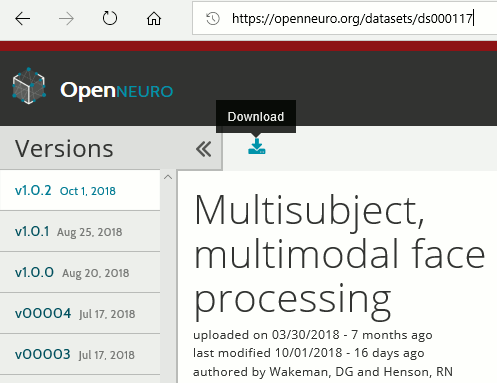
Download the entire dataset from the OpenNeuro website (one single .tar file):
https://openneuro.org/datasets/ds000117/versions/00004
- Expand the .tar files in the same folder:
- Linux/MacOS: Run "tar -vf filename.tar" from a terminal
Windows: Install a free utility (eg. 7zip, WinRAR), right-click on the file.tar > Extract
Reminder: Do not save the downloaded files in the Brainstorm program or database folders
- In this tutorial, we will use only the derivatives folder (85Gb), if you need to make some space on your hard drive you can delete all the other folders. Files we will use here:
FreeSurfer anatomy: /derivatives/freesurfer/sub-XX/ses-mri/anat/*
- MEG recordings (SSS): /derivatives/meg_derivatives/sub-XX/ses-meg/meg/*.fif
- Empty-room (SSS): /derivatives/meg_derivatives/sub-emptyroom/ses-meg/meg/*.fif
Start Brainstorm (Matlab scripts or stand-alone version). For help, see the Installation page.
Select the menu File > Create new protocol. Name it "TutorialVisual" and select the options:
"No, use individual anatomy",
"No, use one channel file per condition".
Import the anatomy
This dataset is formatted following the BIDS-MEG specifications, therefore we could import all the relevant information (MRI, FreeSurfer segmentation, MEG+EEG recordings) in just one click, with the menu File > Load protocol > Import BIDS dataset, as described in the online tutorial MEG resting state & OMEGA database. However, because your own data might not be organized following the BIDS standards, in this tutorial we preferred illustrating all the detailed steps for importing the data rather than the BIDS shortcut. Plus, we will need some additional steps that are not part of the standard import, because of the data anonymization (MRI were defaced and acquisition dates removed).
This page explains how to import and process the first run of subject #01 only. All the other files will have to be processed in the same way.
- Switch to the "anatomy" view.
Right-click on the TutorialVisual folder > New subject > sub-01
- Leave the default options you defined for the protocol.
Right-click on the subject node > Import anatomy folder:
Set the file format: "FreeSurfer folder"
Select the folder: derivatives/freesurfer/sub-01/ses-mri/anat
- Number of vertices of the cortex surface: 15000 (default value)
When asked to select the anatomical fiducials, click on "Compute MNI transformation". This will register the MRI volume to an MNI template with an affine transformation, using SPM functions embedded in Brainstorm (spm_maff8.m). This will also place default fiducial points NAS/LPA/RPA in the MRI, based on MNI coordinates. We will use digitized head points for the MEG-MRI coregistration, therefore we don't need accurate anatomical positions here.
- Note that if you don't have a good digitized head shape for the subject, or if the final registration MEG-MRI doesn't look good with this head shape, you should not skip this step and mark accurate NAS/LPA/RPA fiducial points in the MRI, using the same anatomical convention that was used during the MRI acquisition.
- Then click on [Save] to start the import.
At the end of the process, make sure that the file "cortex_15000V" is selected (downsampled pial surface, that will be used for the source estimation). Otherwise, double-click on it to select it as the default cortex surface. Do not worry about the big holes in the head surface, parts of MRI have been remove voluntarily for anonymization purposes.
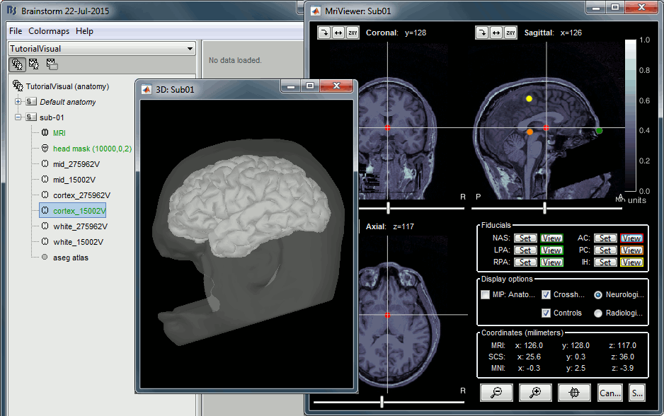
All the anatomical atlases generated by FreeSurfer were automatically imported: the cortical atlases (Desikan-Killiany, Mindboggle, Destrieux, Brodmann) and the sub-cortical regions (ASEG atlas).
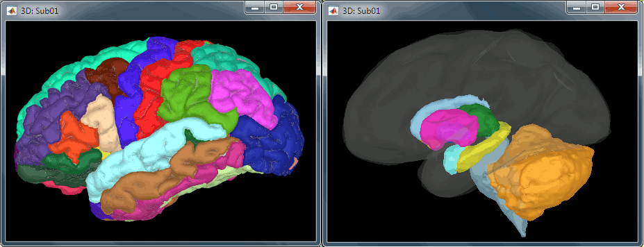
Access the recordings
Link the recordings
We need to attach the continuous .fif files containing the recordings to the database.
- Switch to the "functional data" view.
Right-click on the subject folder > Review raw file.
Select the file format: "MEG/EEG: Neuromag FIFF (*.fif)"
Go to the folder: derivatives/meg_derivatives/sub-01/ses-meg/meg
Select file: sub-01_ses-meg_task-facerecognition_run-01_proc-sss_meg.fif
Events: Ignore. We will read the stimulus triggers later.
Refine registration now? NO
The head points that are available in the FIF files contain all the points that were digitized during the MEG acquisition, including the ones corresponding to the parts of the face that have been removed from the MRI. If we run the fitting algorithm, all the points around the nose will not match any close points on the head surface, leading to a wrong result. We will first remove the face points and then run the registration manually.
Channel classification
A few non-EEG channels are mixed in with the EEG channels, we need to change this before applying any operation on the EEG channels.
Right-click on the channel file > Edit channel file. Double-click on a cell to edit it.
Change the type of EEG062 to EOG (electrooculogram).
Change the type of EEG063 to ECG (electrocardiogram).
Change the type of EEG061 and EEG064 to NOSIG (or any other non-informative type). Close the window and save the modifications.
MRI registration
At this point, the registration MEG/MRI is based only on the three anatomical landmarks NAS/LPA/RPA, which are not even accurately set (we used default MNI positions). All the MRI scans were anonymized (defaced) so all the head points below the nasion cannot be used. We will try to refine this registration using the additional head points that were digitized above the nasion.
Right-click on the channel file > Digitized head points > Remove points below nasion.
(42 points removed, 95 head points left)
Right-click on the channel file > MRI registration > Refine using head points.
MEG/MRI registration, before (left) and after (right) this automatic registration procedure:
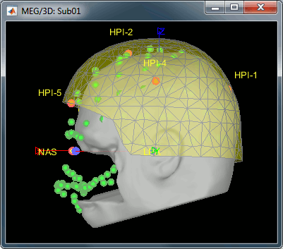
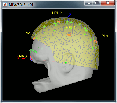
Right-click on the channel file > MRI registration > EEG: Edit.
Click on [Project electrodes on surface], then close the figure to save the modifications.
Read stimulus triggers
We need to read the stimulus markers from the STI channels. The following tasks can be done in an interactive way with menus in the Record tab, as in the introduction tutorials. We will illustrate here how to do this with the pipeline editor, it will be easier to batch it for all the runs and all the subjects.
- In Process1, select the "Link to raw file", click on [Run].
Select process Events > Read from channel, Channel: STI101, Detection mode: Bit.
Do not execute the process, we will add other processes to classify the markers.
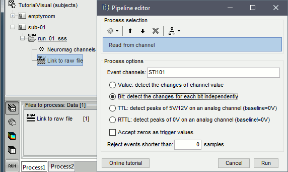
- We want to create three categories of events, based on their numerical codes:
Famous faces: 5 (00101), 6 (00110), 7 (00111) => Bit 3 only
Unfamiliar faces: 13 (01101), 14 (01110), 15 (01111) => Bit 3 and 4
Scrambled images: 17 (10001), 18 (10010), 19 (10011) => Bit 5 only
- We will start by creating the category "Unfamiliar" (combination of events "3" and "4") and remove the remove the initial events. Then we just have to rename the remaining "3" in "Famous", and all the "5" in "Scrambled".
Add process Events > Group by name: "Unfamiliar=3,4", Delay=0, Delete original events
Add process Events > Rename event: 3 => Famous
Add process Events > Rename event: 5 => Scrambled
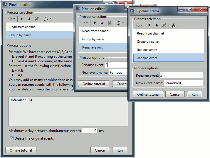
Add process Events > Add time offset to correct for the presentation delays:
Event names: "Famous, Unfamiliar, Scrambled", Time offset = 34.5ms
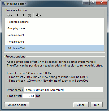
Finally run the script. Double-click on the recordings to make sure the labels were detected correctly. You can delete the unwanted events that are left in the recordings (1,2,9,13). Edit the colors if you don't like the default ones.

Pre-processing
Spectral evaluation
- Keep the "Link to raw file" in Process1.
Run process Frequency > Power spectrum density (Welch) with the options illustrated below.
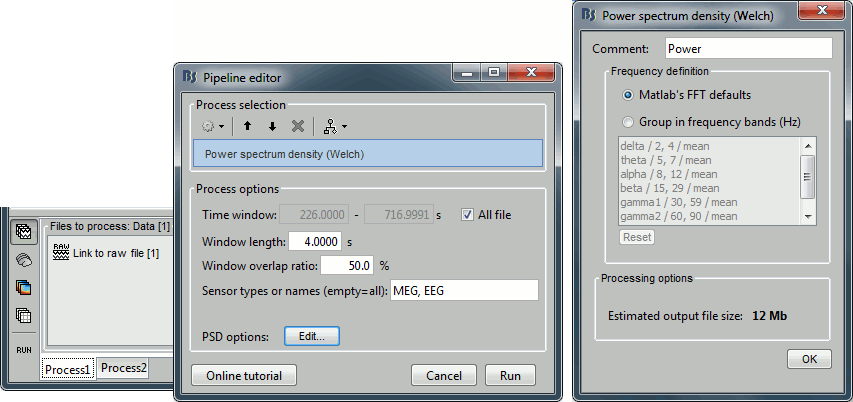
Right-click on the PSD file > Power spectrum.
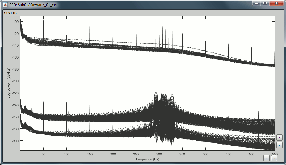
The MEG sensors look awful, because of one small segment of data located around 248s. Open the MEG recordings and scroll to 248s (just before the first Unfamiliar event).
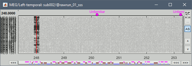
In these recordings, the continuous head tracking was activated, but it starts only at the time of the stimulation (248s) while the acquisition of the data starts 22s before (226s). The first 22s do not have head localization coils (HPI) coils activity and are not corrected by MaxFilter. After 248s, the HPI coils are on, and MaxFilter filters them out. The transition between the two states is not smooth and creates important distortions in the spectral domain. For a proper evaluation of the recordings, we should compute the PSD only after the HPI coils are turned on.
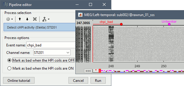
Run process Events > Detect cHPI activity (Elekta). This detects the changes in the cHPI activity from channel STI201 and marks all the data without head localization as bad.
Re-run the process Frequency > Power spectrum density (Welch). All the bad segments are excluded from the computation, therefore the PSD is now estimated only with the data after 248s.
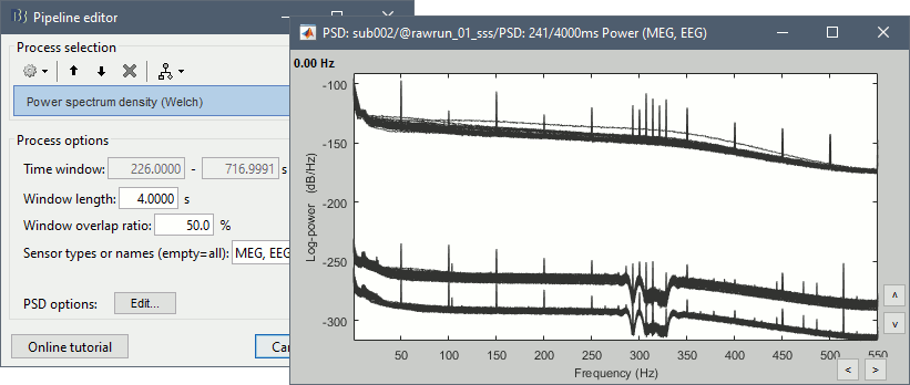
- Observations:
- Three groups of sensors, from top to bottom: EEG, MEG gradiometers, MEG magnetometers.
Power lines: 50 Hz and harmonics
- Alpha peak around 10 Hz
Artifacts due to Elekta electronics (HPI coils): 293Hz, 307Hz, 314Hz, 321Hz, 328Hz.
Peak from unknown source at 103.4Hz in the MEG only.
Suspected bad EEG channels: EEG016
- Close all the windows.
Remove line noise
- Keep the "Link to raw file" in Process1.
Select process Pre-process > Notch filter to remove the line noise (50-200Hz).
Add the process Frequency > Power spectrum density (Welch).
Double-click on the PSD for the new continuous file to evaluate the quality of the correction.
- Close all the windows (use the [X] button at the top-right corner of the Brainstorm window).
EEG reference and bad channels
Right-click on link to the processed file ("Raw | notch(50Hz ...") > EEG > Display time series.
Select channel EEG016 and mark it as bad (using the popup menu or pressing the Delete key).
In the Record tab, menu Artifacts > Re-reference EEG > "AVERAGE".
At the end, the window "select active projectors" is open to show the new re-referencing projector. Just close this window. To get it back, use the menu Artifacts > Select active projectors.
Artifact detection
Heartbeats: Detection
Empty the Process1 list (right-click > Clear list).
- Drag and drop the continuous processed file ("Raw | notch(50Hz...)") to the Process1 list.
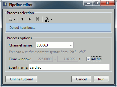
Run process Events > Detect heartbeats: Channel name=EEG063, All file, Event name=cardiac
Eye blinks: Detection
- In many of the other tutorials, we detect the blinks and remove them with SSP. In this experiment, we are particularly interested in the subject's response to seeing the stimulus. Therefore we will exclude from the analysis all the recordings contaminated with blinks or other eye movements.
Run process Events > Detect events above threshold:
Event name=blink_BAD, Channel=EEG062, All file, Maximum threshold=100, Threshold units=uV, Filter=[0.30,20.00]Hz, Use absolute value of signal.
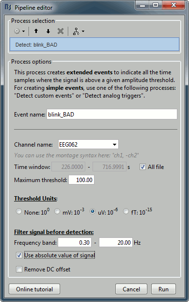
- In other tutorials, we used the process "Detect eye blinks" which creates simple events indicating the peak of the EOG signal during a blink. In this study, we preferred using this process "Detect events above threshold" because it creates extended events marking as bad all the segment for which the EOG value is above a given threshold. It's more manual but it ensures we really exclude all the ocular activity.
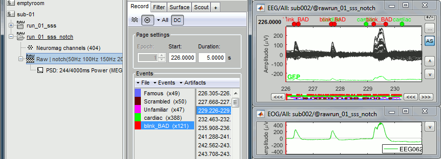
Inspect visually the two new cateogries of events: cardiac and blink_BAD.
- Close all the windows (using the [X] button).
Heartbeats: Correction with SSP
- Keep the "Raw | notch" file selected in Process1.
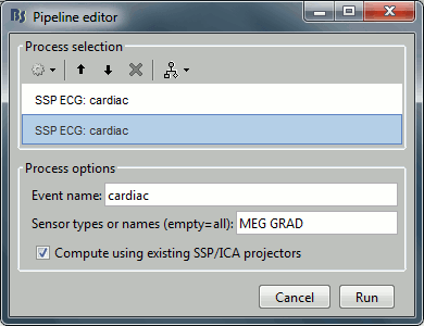
Select process Artifacts > SSP: Heartbeats > Sensor type: MEG MAG
Add process Artifacts > SSP: Heartbeats > Sensor type: MEG GRAD - Run the execution
Double-click on the continuous file to show all the MEG sensors.
In the Record tab, select sensors "Left-temporal".Menu Artifacts > Select active projectors.
In category cardiac/MEG MAG: Select component #1 and view topography.
In category cardiac/MEG GRAD: Select component #1 and view topography.

Make sure that selecting the two components removes the cardiac artifact. Then click [Save].
Additional bad segments
Process1>Run: Select the process "Events > Detect other artifacts". This should be done separately for MEG and EEG to avoid confusion about which sensors are involved in the artifact.
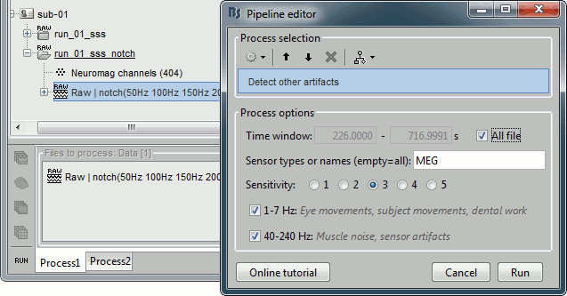
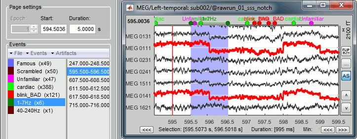
Display the MEG sensors. Review the segments that were tagged as artifact, determine if each event represents an artifact and then mark the time of the artifact as BAD. This can be done by selecting the time window around the artifact, then right-click > Reject time segment. Note that this detection process marks 1-second segments but the artifact can be shorter.

- Once all the events in the two categories are reviewed and bad segments are marked, the two categories (1-7Hz and 40-240Hz) can be deleted.
- Do this detection and review again for the EEG.
SQUID jumps
MEG signals recorded with Elekta-Neuromag systems frequently contain SQUID jumps (more information). These sharp steps followed by a change of baseline value are easy to identify visually but more complicated to detect automatically.
The process "Detect other artifacts" usually detects most of them in the category "1-7Hz". If you observe that some are skipped, you can try re-running it with a higher sensitivity. It is important to review all the sensors and all the time in each run to be sure these events are marked as bad segments.
Epoching and averaging
Import epochs
- Keep the "Raw | notch" file selected in Process1.
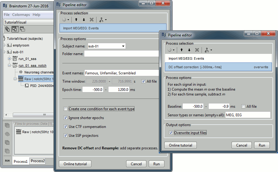
Select process: Import > Import recordings > Import MEG/EEG: Events (do not run immediately)
Event names "Famous, Unfamiliar, Scrambled", All file, Epoch time=[-500,1200]msAdd process: Pre-process > Remove DC offset: Baseline=[-500,-0.9]ms - Run execution.
Average by run
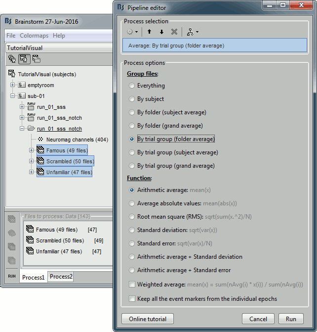
- In Process1, select all the imported trials.
Run process: Average > Average files: By trial groups (folder average)
Review EEG ERP
EEG evoked response (famous, scrambled, unfamiliar), low-pass filter at 32Hz:
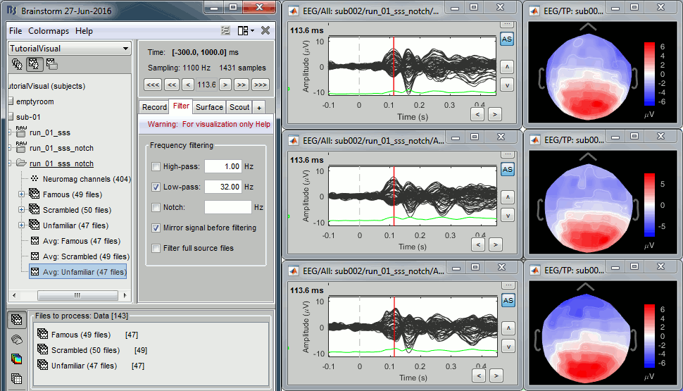
Open the Cluster tab and create a cluster with the channel EEG065 (button [NEW IND]).

Select the cluster, select the three average files, right-click > Clusters time series (Overlay:Files).
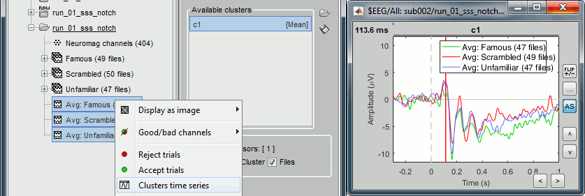
- Basic observations for EEG065 (right parieto-occipital electrode):
- Around 170ms (N170): greater negative deflection for Famous than Scrambled faces.
- After 250ms: difference between Famous and Unfamiliar faces.
Source estimation [TODO]
MEG noise covariance: Empty room recordings [TODO]
The minimum norm model we will use next to estimate the source activity can be improved by modeling the the noise contaminating the data. The introduction tutorials explain how to estimate the noise covariance in different ways for EEG and MEG. For the MEG recordings we will use the empty room measurements we have, and for the EEG we will compute it from the pre-stimulus baselines we have in all the imported epochs.
There are 8 empty room files available in this dataset. For each subject, we will use only one file, the one that was acquired at the closest date. We will now import and process all the empty room recordings simultaneously, even if only one is needed by the current subject. Later, for each subject we will select the most appropriate noise covariance matrix.
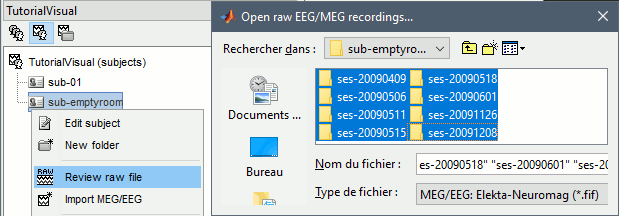
Create a new subject: sub-emptyroom
Right-click on the new subject > Review raw file.
Select all the folders in: derivatives/sub-emptyroom (processed with MaxFilter/tSSS)
Do not apply default transformation, Ignore event channel.
Select all these new files in Process1 and run process Pre-process > Notch filter: 50 100 150 200Hz. When using empty room measurements to compute the noise covariance, they must be processed exactly in the same way as the other recordings (same MaxFilter parameters, same frequency filters).
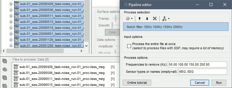
- Delete all the original noise files and keep only the filtered ones.
Identify the noise file that was recorded the closest to the subject's recordings. You can read the acquisition date of a file in the tooptip that is displayed when you leave you mouse for a while over its folder. The MEG for subject sub-01 was recorded on April 9th 2009, so we will compute the MEG noise covariance for this subject from the first noise file available, which was acquired on the same date.
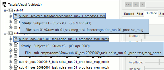
Right-click on the noise recordings 2009-04-09 > Noise covariance > Compute from recordings:
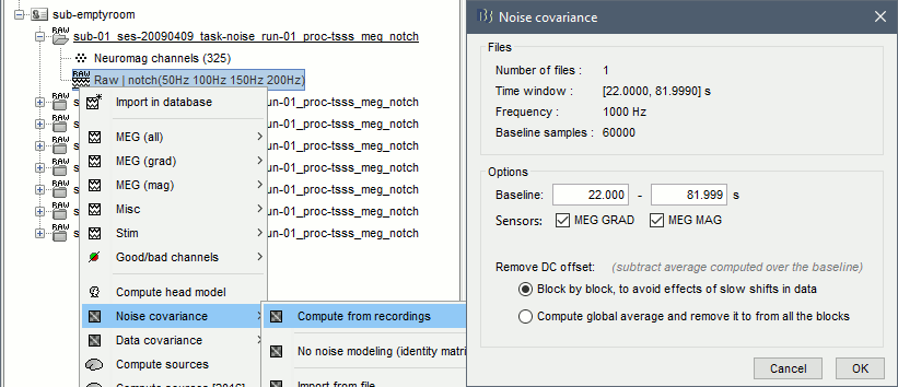
Finally copy the noise covariance from sub-emptyroom to the folder with imported epochs in sub-01. Use the popup menus File>Copy/Paste, or the keyboard shortcuts Ctrl+C/Ctrl+V.
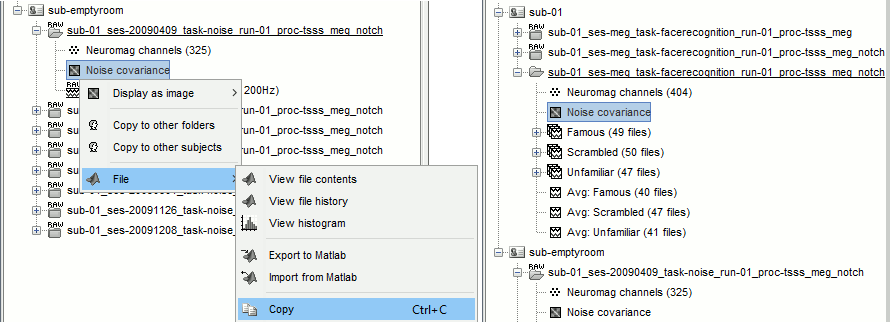
EEG noise covariance: Pre-stimulus baseline
In folder sub-01/run-01_tsss_notch, select all the imported the imported trials, right-click > Noise covariance > Compute from recordings, Time=[-500,-0.9]ms, EEG only, Merge.
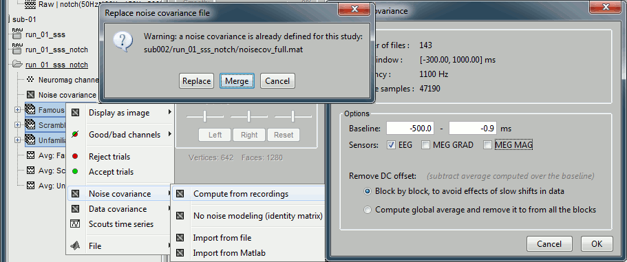
This computes the noise covariance only for EEG, and combines it with the existing MEG information.
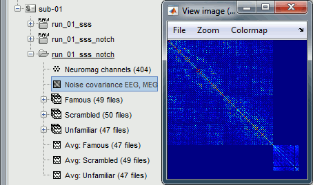
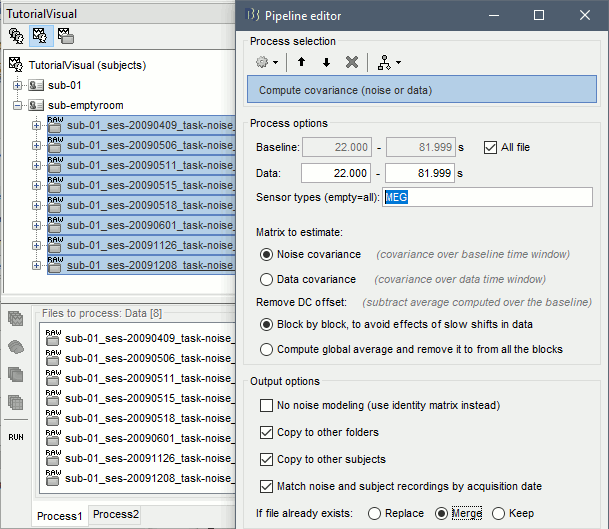
To generate the corresponding analysis script, we will use a different strategy, which will match automatically the subject with the appropriate MEG noise covariance. We will first import all the subjects, compute the EEG noise covariance for all the runs, then compute the MEG noise covariance matrix for all the empty room files at once with the process "Sources > Compute covariance" with the options "Match noise and subject recordings by acquisition date", "Sensor types=MEG", "Merge".
BEM layers
We will compute a BEM forward model to estimate the brain sources from the EEG recordings. For this, we need some layers defining the separation between the different tissues of the head (scalp, inner skull, outer skull).
- Go to the anatomy view (first button above the database explorer).
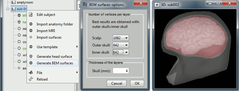
Right-click on the subject folder > Generate BEM surfaces: The number of vertices to use for each layer depends on your computing power and the accuracy you expect. You can try for instance with 1082 vertices (scalp) and 642 vertices (outer skull and inner skull).
Forward model: EEG and MEG
- Go back to the functional view (second button above the database explorer).
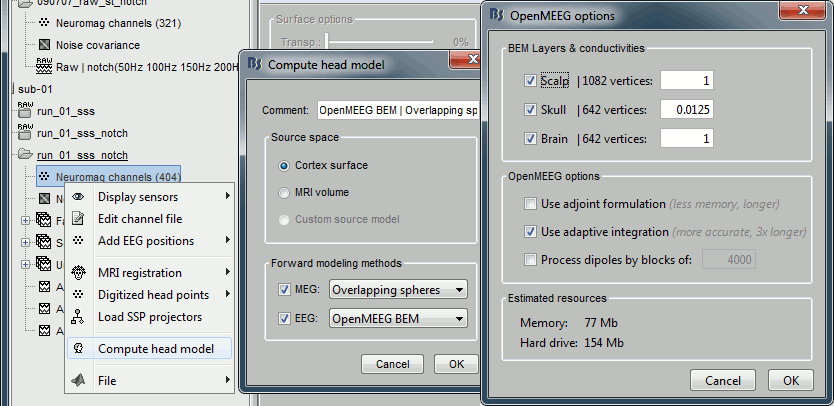
Model used: Overlapping spheres for MEG, OpenMEEG BEM for EEG (more information).
In folder sub-01/run_01_tsss_notch, right-click on the channel file > Compute head model.
Keep all the default options . Expect this to take a while...
Inverse model: Minimum norm estimates
Right-click on the new head model > Compute sources [2016]: MEG MAG + GRAD (default options)
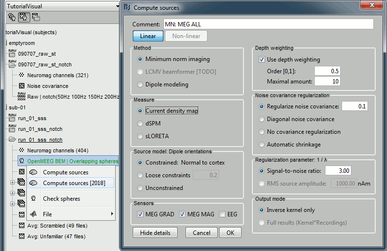
Right-click on the new head model > Compute sources [2016]: EEG (default bad channels).
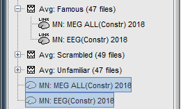
At the end we have two inverse operators, that are shared for all the files of the run (single trials and averages). If we wanted to look at the run-level source averages, we could normalize the source maps with a Z-score wrt baseline. In this tutorial, we will first average across runs and normalize the subject-level averages. This will be done in the next tutorial (group analysis).
Time-frequency analysis
We will compute the time-frequency decomposition of each trial using Morlet wavelets, and average the power of the Morlet coefficients for each condition and each run separately. We will restrict the computation to the MEG magnetometers and the EEG channels to limit the computation time and disk usage.
- In Process1, select the imported trials "Famous" for run#01.
Run process Frequency > Time-frequency (Morlet wavelets): Sensor types=MEG MAG,EEG
Not normalized, Frequency=Log(6:20:60), Measure=Power, Save average
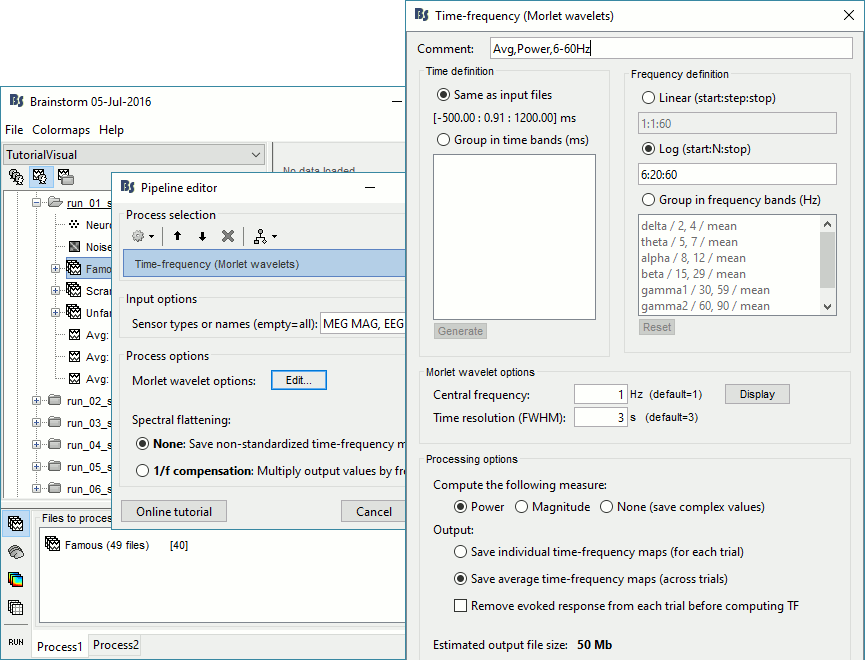
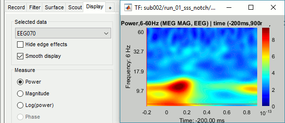
Double-click on the file to display it. In the Display tab, select the option "Hide edge effects" to exclude from the display all the values that could not be estimated in a reliable way. Let's extract only the good values from this file (-200ms to +900ms).
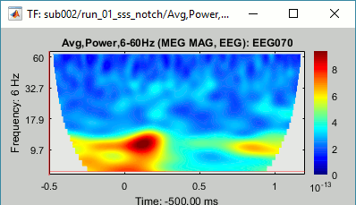
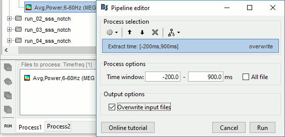
- In Process1, select the time-frequency file.
Run process Extract > Extract time: Time window=[-200, 900]ms, Overwrite input files
Display the file again, observe that all the possibly bad values are gone.
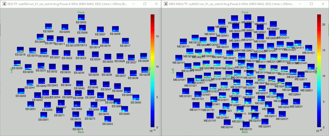
You can display all the sensors at once (MEG MAG or EEG): right-click > 2D Layout (maps).
- Repeat these steps for other conditions (Scrambled and Unfamiliar) and the other runs (2-6). There is no way with this process to compute all the averages at once, as it is with the process "Average files". This will be easier to run from a script.
- If we wanted to look at the run-level source averages, we could normalize these time-frequency maps. In this tutorial, we will first average across runs and normalize the subject-level averages. This will be done in the next tutorial (group analysis).
Scripting
We have now all the files we need for the group analysis (next tutorial). We need to repeat the same operations for all the runs and all the subjects. Some of these steps are fully automatic and take a lot of time (filtering, computing the forward model), they should be executed from a script.
However, we recommend you always review manually some of the pre-processing steps (selection of the bad segments and bad channels, SSP/ICA components). Do not trust blindly any fully automated cleaning procedure.
For the strict reproducibility of this analysis, we provide a script that processes all the 19 subjects: brainstorm3/toolbox/script/tutorial_visual_full_single.m (execution time: 10-30 hours)
Report for the first subject: report_TutorialVisual_sub-01.html
You should note that this is not the result of a fully automated procedure. The bad channels were identified manually and are defined for each run in the script. The bad segments were detected automatically, confirmed manually for each run and saved in external files, then exported as text ans copied at the end of this script.
All the process calls (bst_process) were generated automatically using with the script generator (menu Generate .m script in the pipeline editor). Everything else was added manually (loops, bad channels, file copies).

