|
Size: 38534
Comment:
|
Size: 26413
Comment:
|
| Deletions are marked like this. | Additions are marked like this. |
| Line 1: | Line 1: |
| = Yokogawa/KIT recordings = ''Authors: Francois Tadel, Ei-ichi Okumura, Takashi Asakawa.'' |
= Yokogawa/KIT tutorial = ''Authors: Francois Tadel, Yasuhiro Haruta, Ei-ichi Okumura, Takashi Asakawa'' |
| Line 9: | Line 9: |
| This tutorial dataset (EEG and MRI data) remains proprietary of the Epilepsy Centre, University Hospital Freiburg, Germany. Its use and transfer outside the Brainstorm tutorial, e.g. for research purposes, is prohibited without written consent from the Epilepsy Center in Freiburg. For questions please contact A. Schulze-Bonhage, MD, PhD: andreas.schulze-bonhage@uniklinik-freiburg.de == Presentation of the experiment == Unilateral median nerves were percutaneously stimulated using monophasic square-wave impulses with a duration of 0.3 ms at 2.8 Hz. The stimulus intensity was set at the motor threshold to evoke mild twitches of the thumb. The stimulus onsets were recorded as low-to-high TTL with a trigger channel labeled as "Trigger01". The total number of stimuli in the dataset was 336. == Overview of the data processing == 1. Yokogawa/KIT data In importing Yokogawa/KIT data files (“.con”, “.raw”, and “.ave”) into Brainstorm, a data export process is required beforehand. The data export function is available in Meg160, which is data analysis software equipped in most of Yokogawa/KIT systems (*1). 2. Preparation If a wave data file and the corresponding digitizer file are ready for use, there is no additional operation required. Please go to “3. Data export”. If no digitizer file is available, the following operation is required: Extraction of Head Surface Points Select the [Surface Point File] menu from [BESA Text Export] under [Import and Export] in the [File] menu. Check that the fiducial points are properly pointed, and then click the [OK] button. A surface point file (“.sfp”), which includes position data of fiducial points, marker points, and other points describing the head shape, is automatically created. 3. Data export Select the [Third-Party Export] menu under [Import and Export] in the [File] menu, and then an operation panel for data export will show up (*1, *2). The next procedure depends on the availability of the digitizer data: When using digitizer data: In the operation panel, select [Digitizer] and provide the digitizer file and the label file in the [Point Filename] box and the [Label Filename] box, respectively. The point file is a “.txt” file generally available under the corresponding “Scan” folder, and the label file is “DigitizeLabel.txt” generally located in the “C:¥Meg160¥AppInfo” folder. Finally, provide an output file name in [Third-party Export Dataset], and then push the [Create Export File] button. Use this exported file in Brainstorm. When using surface point data instead: In the operation panel, select [Surface Point File] and provide the surface point file (“.sfp”) created in “Extraction of Head Surface Points”. Finally, provide an output file name in [Third-party Export Dataset], and then push the [Create Export File] button. Use this exported file in Brainstorm. (*1): If your software does not support this function, please contact Yokogawa via http://www.yokogawa.com/me/index.htm. (*2): In some systems, the function name reads [BESA Binary Export] instead of [Third-party Export]. |
This tutorial dataset (MEG/EEG and MRI data) remains proprietary of Yokogawa Electric Corporation, Japan. Its use and transfer outside the Brainstorm tutorial, e.g. for research purposes, is prohibited without written consent from Yokogawa Electric Corporation. == Description of the experiment == This tutorial is based on a simple median nerve stimulation experiment: * Right median nerves were percutaneously stimulated using monophasic square-wave impulses with a duration of 0.3 ms at 2.8 Hz. * The stimulus intensity was set at the motor threshold to evoke mild twitches of the thumb. * The stimulus onsets were recorded as low-to-high TTL with a trigger channel labeled as "Trigger01". * The total number of stimuli in the dataset was 336. * The MEG data was recorded with a sampling rate of 2000 Hz and a bandpass filter at 0.16-500 Hz with a Yokogawa 160 axial gradiometer system at Yokogawa Electric Corporation, Kanazawa, Japan. * The EEG data was recorded with a NIHON KOHDEN system simultaneously with the MEG recordings. == Export recordings from Meg160 == To import Yokogawa/KIT data files (.con, .raw, .ave) into Brainstorm, a data export process is required beforehand. The data export function is available in Meg160, which is data analysis software equipped in most of Yokogawa/KIT systems. The dataset used in this tutorial has already been exported using this procedure. It is described here so that later you can export your own recordings to Brainstorm. If your software does not support the functions used below, please contact Yokogawa via<<BR>> http://www.yokogawa.com/me/index.htm '''Export the digitizer file''' * If a wave data file and the corresponding digitizer file are ready for use, there is no additional operation required. * If no digitizer file is available, you need first to extract the head surface points: * In Meg160, select the menu: File > Import and Export > BESA Text Export > Surface Point File * Check that the fiducial points are properly pointed, and then click the [OK] button * A surface point file (.sfp) is automatically created. It includes the position data of: the fiducial points, the marker points and other points describing the head shape ==== Full head shape in the the digitizer file ==== In order to realize a precise MRI registration or for warping the default anatomy ([[Tutorials/TutWarping|see tutorial]]), you should collect 100 to 200 points describing the entire head shape in addition to the 8 Yokogawa/KIT standard stylus points. To import additional digitized points, follow the instruction below: * When digitizing head points: * Pick the 8 standard stylus points * Pick additional 100 to 200 head points, so that the selected points cover the entire head * Edit the digitizer label file (DigitizeLabel.txt) which is used in "Third-party export" so that it defines the 8 points and the additional points. * Note that the number of additional labels should be >= the number of digitized points. * As for the new label names, any names can be used if the names are not duplicated. * The following is an example: {{{ fidt9 HPI_1 HPI_4 HPI_3 HPI_5 HPI_2 fidt10 fidnz ETC001 ETC002 ETC003 ... ETC[nnn] }}} * Where [nnn]+8 should be >= the number of digitized points. * Use the modified digitizer label file with the digitizer data in the "Third-party export" function. '''Export the recordings''' * In Meg160, select the menu: File > Import and Export > Third-Party Export * On some systems, this menu is name [BESA Binary Export] * An operation panel for data export shows up * When using digitizer data: * Select [Digitizer] * Enter the digitizer file in the [Point Filename] box<<BR>>(.txt file generally available under the corresponding "Scan" folder) * Enter the label file in the [Label Filename] box<<BR>>(DigitizeLabel.txt generally located in the "C:\Meg160\AppInfo" folder) * When using surface point data instead: * Select [Surface Point File] * Enter the surface point file (.sfp) created previously. * Enter an output file name in [Third-party Export Dataset] * Click on [Create Export File] * Use this exported file in Brainstorm |
| Line 21: | Line 83: |
| * Unzip it in a folder that is __not__ in any of the Brainstorm folders (program folder or database folder) | * Unzip it in a folder that is __not__ in any of the Brainstorm folders (program or database folder) |
| Line 23: | Line 85: |
| * Select the menu File > Create new protocol. Name it "'''!TutorialYokogawa'''" and select the options: | * Select the menu File > Create new protocol. Name it "'''TutorialYokogawa'''" and select the options: |
| Line 25: | Line 87: |
| * "'''Yes, use one channel file per subject'''". | * "'''No, use one channel file per condition'''". |
| Line 28: | Line 90: |
| * Right-click on the !TutorialEpilepsy folder > New subject > '''sepi01''' | * Right-click on the TutorialYokogawa folder > New subject > '''Subject01''' |
| Line 31: | Line 93: |
| * Set the file format: "!FreeSurfer folder" * Select the folder: '''sample_epilepsy/anatomy''' |
* Set the file format: "FreeSurfer folder" * Select the folder: '''sample_yokogawa/anatomy''' |
| Line 35: | Line 97: |
| * NAS: x=135, y=222, z=75 * LPA: x=57, y=118, z=68 * RPA: x=204, y=119, z=76 * AC: x=131, y=145, z=110 * PC: x=130, y=119, z=111 * IH: x=128, y=134, z=170 (anywhere on the midsagittal plane) * At the end of the process, make sure that the file "cortex_15000V" is selected (downsampled pial surface, that will be used for the source estimation). If it is not, double-click on it to select it as the default cortex surface.<<BR>><<BR>> {{attachment:anatomy.gif||height="257",width="442"}} |
* NAS: x=128, y=227, z=93 * LPA: x=48, y=130, z=69 * RPA: x=214, y=130, z=76 * AC: x=128, y=148, z=116 * PC: x=128, y=123, z=117 * IH: x=128, y=131, z=176 (anywhere on the midsagittal plane) * At the end of the process, make sure that the file "cortex_15000V" is selected (downsampled pial surface, which will be used for the source estimation). If it is not, double-click on it to select it as the default cortex surface.<<BR>><<BR>> {{attachment:anatomy.gif||height="195",width="346"}} |
| Line 44: | Line 106: |
| If you do not have access to an individual MR scan of the subject (or if its quality is too low to be processed with !FreeSurfer), but if you have digitized the head shape of the subject using a tracking system, you have an alternative: deform one of the Brainstorm templates (Colin27 or ICBM152) to match the shape of the subject's head.<<BR>>For more information, read the following tutorial: [[Tutorials/TutWarping|Warping default anatomy]] | If you do not have access to an individual MR scan of the subject (or if its quality is too low to be processed with FreeSurfer), but if you have digitized the head shape of the subject using a tracking system, you have an alternative: deform one of the Brainstorm templates (Colin27 or ICBM152) to match the shape of the subject's head.<<BR>>For more information, read the following tutorial: [[Tutorials/TutWarping|Warping default anatomy]] |
| Line 50: | Line 112: |
| * Select the file format: "EEG: Deltamed Coherence-Neurofile(*.bin)" * Select the file: '''sample_epilepsy/data/tutorial_eeg.bin''' * The new file "Link to raw file" lets you access directly the contents of the EEG recordings * The channel file "Deltamed channels" in the (Common files) folder contains the name of the channels, but not their positions. We need to overwrite this file and import manually the positions of the electrodes (either a standard cap or accurate positions digitized with a Polhemus device). |
* Select the file format: "MEG/EEG : Yokogawa/KIT" * Select the file: '''sample_yokogawa/data/SEF_000-export.con''' * Answer '''NO''' when asked to refine the registration using head points. In this dataset, we only have access to the positions of the electrodes and three additional markers on the forehead. The automatic registration doesn't work well in this case, we are going to fix this registration manually. * A figure is opened to show the current registration MRI/MEG. It is already quite good, but can be improved a bit manually. Close this figure. * The new file "Link to raw file" lets you access directly the contents of the MEG/EEG recordings * The channel file "KIT channels" contains the name of the channels and the position of the corresponding sensors. <<BR>> {{attachment:review_raw.gif||height="157",width="416"}} |
| Line 56: | Line 121: |
| * Right-click on the subject folder > Import channel file: * Select the file format: "EEG: ANT Xensor (*.elc)" * Select the file: '''sample_epilepsy/data/tutorial_electrodes.elc''' * Confirm that you want to overwrite the existing channel file. * This file contains the default electrodes positions from the ASA software (ANT) |
|
| Line 62: | Line 122: |
| * 29 EEG electrodes * EOG1, EOG2: Electrooculograms * EMG, ECG: Electromyogram and electrocardiogram * SP1, SP2: Sphenoidal electrodes * RS: Electrode on the right shoulder * PHO: Photo stimulation channel * DELR, DELL, QR, QL: Additional * The file format for the electrodes positions does not describe the type of the channels correctly, therefore all the signals saved in the files are classified as EEG. We need to redefine this manually to get correct groups of sensors, we want to have only real EEG electrodes in the "EEG" category and put everything that we are not going to use a "MISC" category. * Right-click on the channel file > Edit channel file: * Note that the EOG, EMG and ECG channels already have a different type * Select all the other non-EEG channels: SP1, SP2, RS, PHO, DELR, DELL, QR, QL * Right-click in the window > Set channel type: type '''MISC''' |
* 160 MEG channels * 12 MEG references * 14 Trigger channels * 41 EEG channels * 2 EOG channels: EO1 and EO2 * 1 ECG channel: EKG+ * 1 ground of the EEG amplifier: E * Not all the types of channels are properly identified in Brainstorm. We need to redefine this manually to get correct groups of sensors. * Right-click on the channel file > '''Edit channel file''': * Channel EO1 (208) and EO2 (209): Change the type to '''EOG''' * Channel EKG+ (214): Change the type to '''ECG''' * Channel E (231): Change the type to '''MISC''' |
| Line 76: | Line 137: |
| {{attachment:channel_type.gif}} ==== Register electrodes with MRI ==== * The channel file we imported contains generic electrodes positions; hence, it cannot be fully aligned with the head surface coming from the MRI. We need to register manually these electrodes positions with the subject anatomy. * Right-click on the channel file > MRI registration > Edit... You will see several buttons across the toolbar; to get the function of a button, hover your mouse for a few seconds over it to reveal the tooltip. * You can click on the "Label" button in the toolbar to show the electrode names. The default positions are already quite good, and the head shape is correct; only limited manual registration will be required in the next few steps. * Click on the button "Refine registration using head points" to find a better registration between the head shape defined by the electrodes and the head surface coming from the MRI. * Click on the button "Project electrodes on scalp surface", to ensure all the electrodes touch the skin surface. * Click on "OK" and agree to save the modifications.<<BR>><<BR>> {{attachment:channel_align.gif|channel_type.gif|height="191",width="352"}} == Review EEG recordings == ==== Import the spike markers ==== Some spikes were marked by the epileptologists at the Epilepsy Center in Freiburg with Brainstorm and saved in an external text file. We are going to import this file manually. * Right-click on the "Link to raw file" > EEG > Display time series. * In the tab Record, menu File > Add events from files... * Select file format "Array of times" (We are importinga a text file containing the timing of the markers) * Select file '''sample_epilepsy/data/''''''tutorial_spikes.txt''' * When prompted, enter the event name "'''SPIKE'''" * Note that a new category SPIKE is visible in the events list, containing 58 markers * Close the viewer and agree to save the modifications ==== Display the recordings in one montage ==== * For basic information on how to manipulate the montages in Brainstorm: [[http://%20neuroimage.usc.edu/brainstorm/Tutorials/TutExploreRecodings#Montages|read this tutorial]]. * Open a time series figure with the "'''Average reference'''" montage * Right-click on the "Link to raw file" > EEG > Display time series. * In the Record tab, select the first button in the toolbar (Display mode for time series) to view the signals in columns. * Select the "Average reference" in the drop-down list. This menu allows you to set a predefined montages to linearly re-arranging the waveforms. Note the keyboard shortcuts in the menus. * In the Record tab, change the default duration that is reviewed to '''10s'''. * In the figure, click on the '''[Flip +/-]''' button to have the negative values pointing up (convention used by most neurologists) * Open a '''2D Sensor cap''' map of the EEG sensor values as well: * Right-click on "Link to raw file" again > EEG > '''2D Sensor cap ''' * In the Record tab, set the Montage to this view to "'''Average reference'''" * Open the '''ECG '''and '''EOG '''traces as well, to avoid confusing spikes with cardiac or ocular artifacts:<<BR>> * Right-click on the Link to raw file > ECG > Display time series * Right-click on the Link to raw file > EOG > Display time series * The ECG is almost mandatory. The EOG is optional: it can be helpful for beginners but an experienced reviewer will easily recognize the eye movements directly in the EEG data. * Re-arrange the figures in a convenient way, for example as illustrated below, and disable the automatic positioning of the figures you the figure arrangement doesn't get lost when you open a new figure (Window layout menu at the top-right of the Brainstorm figure > None) * Having a lot of windows open may slow down significantly the display because each time you change the current time, all the figures have to be updated. A lot of space is also wasted on the screen due to window frames. The number of windows to open has to be a balance between the amount of information to display and the ease of use. * Review a few existing SPIKE events, to get the feeling of how this reviewing environment works. {{attachment:reviewall.gif}} ==== Frequency filters ==== Go to the Filter tab to enable some display frequency filters. General recommendations are: * High-pass filter: '''0.5 Hz''' * Low-pass filter: '''70 Hz'''<<BR>><<BR>> {{attachment:filters.gif||height="175",width="205"}} ==== Time and amplitude resolution ==== The resolutions of the time and amplitude axes has a lot of importance for the visual detection of epileptic spikes. The shapes we are looking for are altered by the horizontal and vertical scaling. The distance unit on a screen is the pixel, we can set how much time is represented by one pixel horizontally and how much amplitude is represented by one pixel vertically. In the Brainstorm interface, this resolution is usually set implicitly: you can set the size of the window, the duration or recordings reviewed at once (text box "duration" in tab Record) and the maximum amplitude to show in the figure (buttons [...] and [AS] on the right of the time series figure). From there, you can also zoom in time ([<], [>], mouse wheel) or amplitude (['''^'''], [v], Shift+mouse wheel). Those parameters are convenient to explore the recordings interactively but don't allow us to have reproducible displays with constant time and amplitude resolutions. To set the figure resolution explicitly: right-click on the figure > Figure > Set axes resolution. Note that this interface does not store the input values, it just modifies the other parameters (figure size, time window, max amplitude) to fit the resolution objectives. Then if you modify those parameters (resize the figure, leave the button [AS] selected and scroll in time, etc) the resolution is lost, you have to set it again manually. Recommendations for this dataset are: * Time axis: '''170 pixels/sec''' (~55 mm/sec) * Amplitude: '''15 μV/pixels''' (~45 μV/mm)<<BR>><<BR>> {{attachment:resolution.gif||height="249",width="595"}} ==== User setups ==== This preparation of the reviewing environment requires a large number of operations, and would become quickly annoying if you have to repeat it every time you open a file. This is a good time to use the menu "User setups" to save this window configuration, to reload it in one click later. In the menu "Window layout", at the top-right of the Brainstorm window, select User setup > New setup. Enter a name of your choice for this particular window arrangement. This operation will also disable the automatic window arrangement (Window layout > None). To reload it later, open one figure on the dataset you want to review and then select your new entry in the User setup menu. . {{attachment:usersetup.gif||height="251",width="347"}} ==== Multiple montages ==== It may be interesting for some cases to display different groups of sensors in multiple windows (eg. with an MEG system with 300 sensors), or some complicated epilepsy cases where you would like to review at the same time multiple montages (eg. longitudinal and transversal bipolar montages). Brainstorm offers a flexible way of doing this. * Open your full reviewing environment as described before, where the EEG signals are displayed with the "'''Average reference'''" montage. * Open another view on the same data with the "'''Longitudinal 3'''" montage ("double-banana" LB-18.3) * Right-click on the "Link to raw file" again > EEG > Display time series * Alternatively, you can right-click on the existing figure > Figure > Clone figure. * Then set the montage for this new figure to "Longitudinal 3" * Redimension all the figures to make room for the new window * Save this as a new "User setup" * If you don't see the "Longitudinal 3" menu, it is probably because you have using Brainstorm before those predefined montages were made available in the software distribution. To add them manually: * In the Record tab, select "Edit montages" in the drop-down menu * Click on the "Load montage" button * Go to the folder "brainstorm3/toolbox/sensors/private/", and select the first file * Note that a new entry (probably "Longitudinal 1") is added to the list of available montages * Repeat the operation with all the files in the folder "brainstorm3/toolbox/sensors/private/" * Click on "Save" to close the montage editor and now select "Longitudinal 3" {{attachment:reviewall2.gif}} == Mark spikes == In this dataset, some single spikes have already been identified by experts at the University Hospital of Freiburg. You can see that 58 SPIKE events are available in the Record tab. Click on a few of them and try to identify the shape of the spike. The procedure if you are marking the events by yourself is the following: * Close all the current figures ("Close all" button at the top-right corner of the Brainstorm window) * Double-click on the "Link to raw file" to open a continuous file viewer, and load your reviewing environment (menu User setups) * Start by creating a group of events (Events > Add group), and select it in the list of events. * Make sure that the time and amplitude resolutions are what you are used to<<BR>>(right-click on the figure > Figure > Set axes resolution) * Scroll through the recordings using the [<<<] and [>>>] buttons or shortcuts such as F3 or F4 (complete list and descriptions available when you leave your mouse over those buttons). * You can adjust the gain of the electrodes to observe better an event with the buttons ['''^'''] and [v] or the shortcut [Shift+mouse wheel]. * When you identify a spike, click in a white area of the figure in order to place the time cursor at the peak of the spike. If you click on the signal itself, it selects the corresponding channel, but you can use the shortcut Shift+Click to prevent this behavior and force the time cursor to be moved instead. * Press Ctrl+E to add a marker where the time cursor is. * If you are marking multiple types of events, it is convenient to set up some additional keyboard shortcuts. Using the menu '''Events > Edit keyboard shortcuts''', you can associate custom events to the key 1 to 9 of the keyboard. Define the name of the event type to create for each key, and then simply press the corresponding key to add/delete a marker at the current time position. * To jump to the next/previous event in the current category: use the keyboard shortcuts [Shift+arrow right] and [Shift+arrow left] * More information on the data viewer, see tutorial: [[Tutorials/TutRawViewer|Review continuous recordings]]. == Pre-process recordings == |
<<BR>> {{attachment:edit_channel.gif||height="167",width="512"}} ==== Refine the MRI registration ==== * Right-click on the channel file > MRI registration > Edit... (EEG) * The white points are the electrodes, the green points are the additional digitized head points. To display the label of the electrodes, click on the [LABEL] button in the toolbar. To see what the other buttons in the toolbar are doing and how to use them, leave your mouse over them for a few seconds and read the description. * Now try to manipulate the position of the EEG+MEG sensors using '''rotations '''and '''translations '''only (no "resize" or individual electrodes adjustments). The objective is to have all the points close to the surface and the three forehead points inside the little peaks on the surface (due to markers in the MRI). * The rotation+translation are going to be applied both to the EEG and the MEG sensors. After you are done with this solid registration part, you can click on the button '''"Project electrodes on scalp surface"''', it will help for the source modeling later. The green points (digitized) stay in place, the white points (electrodes) are now projected on the skin of the subject. * If you feel like you made it wrong, close the figure and cancel the modifications, then try again. It takes a few trials to get used to this rotation/translation interface. * Click on '''[OK]''' when done. * Answer '''YES''' to save the modifications. * Answer '''YES''' again to apply the solid transformation (rotation+translation) to the MEG sensors. * Before manual registration: <<BR>><<BR>> {{attachment:align_before.gif}} * After manual registration: <<BR>><<BR>> {{attachment:align_after.gif}} ==== Read the stimulation information ==== * Right-click on the "Link to raw file" > Trigger > Display time series * In the Record tab, switch to a column view of the sensors (first button in the toolbar) * You can see that all the trigger lines are flat except for "Trigger01", which contains the information of the electric stimulation. We are going to read this trigger channel and convert it to a list of events. Close this figure.<<BR>><<BR>> {{attachment:triggers_display.gif||height="165",width="447"}} * Drag and drop the "Link to raw file" in the Process1 box. * Run the process "'''Import recordings > Read from channel'''" * Event channel = '''Trigger01''' * Option selected "'''TTL'''": detect peaks of 5V/12V on an analog channel * Do not select the option Accept zeros as trigger values<<BR>><<BR>> {{attachment:triggers_read.gif||height="260",width="302"}} * Right-click on the "Link to raw file" > Trigger > Display time series. Check that the peaks of the triggers channel have been correctly identified, then close this figure.<<BR>><<BR>> {{attachment:triggers_check.gif||height="162",width="369"}} == Artifacts: Evaluate the power spectrum == |
| Line 190: | Line 166: |
| * Drag the "Link to raw file" to the Process1 box and run the process "Frequency > Power spectrum density (Welch)". Configure it as illustrated in the following figure (window length=10s, overlap=50%).<<BR>><<BR>> {{attachment:psd1.gif||height="281",width="312"}} * Double-click on the new PSD file to display it.<<BR>><<BR>> {{attachment:psd2.gif||height="199",width="388"}} * The sharp drop we observe at 50Hz on all the electrodes indicates that a notch filter was already applied to the data, we do not need to remove the power line contamination again. If we had to, we would run the process "Pre-processing > Sinusoid removal (notch)" as explained in the tutorial [[Tutorials/TutRawSsp|Detect and remove artifacts]]. ==== High-pass filter ==== We would like to apply a 0.5Hz high-pass filter to the entire file in order to get rid of the long amplitude fluctuations (longer than 2s). With some MEG file formats, Brainstorm supports the creation of new filtered files in native formats, which means that you can drag and grop directly the "Link to raw file" to the Process1 tab and run the band-pass filter process. Unfortunately, this is currently not supported for the file format we are currently working on (Deltamed Coherence-Neurofile). There is an alternative option which consists in importing the entire continuous file in the database in one single block, then run the filter on it. This approach works is possible only on rather small files (4 * file size < memory on the computer). Here the file size is less than 80 Mb, so it can be easily processed this way. * Right-click on the "Link to raw file" > Import in database. * Uncheck all the options and leave the default "Time window" option. <<BR>><<BR>> {{attachment:import_all.gif||height="295",width="490"}} * Click on Import, it creates an integral copy of the file in the database. Do NOT try to review it: for imported file, the partial loading and the scrolling in time are disabled and it would take a lot of time to display the waveforms for the entire file. It could event result in a crash of Brainstorm or Matlab. * Drag this new file "Raw (0s,3600s)" to the Process1 * Run the process "Pre-process > Band-pass filter", with the options: * Lower cutoff frequency: '''0.5Hz''' (high-pass filter at 0.5Hz) * Upper cutoff frequency: '''0Hz''' (no low-pass filter) * Mirror signal before filtering: '''On''' * Sensor types: '''EMPTY '''(to process all the signals) * Overwrite: '''On''' (we don't need to keep the original copy)<<BR>><<BR>> {{attachment:bandpass.gif||height="284",width="494"}} |
* Drag the "Link to raw file" to the Process1 box and run the process "'''Frequency > Power spectrum density (Welch)'''". Configure it as illustrated in the following figure:<<BR>>Time window: '''[0,50] s''', Window length: '''4s''', Overlap='''50%'''.<<BR>><<BR>> {{attachment:psd_process.gif||height="289",width="313"}} * Double-click on the new PSD file to display it.<<BR>><<BR>> {{attachment:psd_result.gif||height="183",width="394"}} * The lines on the top represent the EEG electrodes, the lines at the bottom the MEG sensors. If you want to get clearer plots, you can calculate separately the spectrum for the two types of sensors separately, by running twice the process "Power spectrum density" , once with sensor types = "MEG" and once with "EEG", instead of running in on both at the same time like we did. * Observations (below 250Hz): * Peak around 11Hz: Alpha waves from the subject's brain * Peaks at 60Hz, 120Hz, 180Hz, 240Hz on EEG + MEG: <<BR>>Electric contamination due to the power lines (60Hz+harmonics) * Peaks at 35Hz, 65Hz, 70Hz, 183Hz, 197Hz on MEG only: <<BR>>Electric noise coming from an unknown source * MEG sensor '''LC11 '''(in red) appears to have a higher level of noise than all the other MEG sensors, we will check this when review the MEG recordings and probably tag it as a bad channel. ==== Correction ==== * From the Yokogawa software: * Users can apply digital filtering to the data before exporting them to Brainstorm. Depending on the data size and degrees of filter parameters, it sometime takes a very long time. * From Brainstorm: * There is no easy way to process the Yokogawa files at this time using the Brainstorm software. This capability might be added in the future, in which case the procedure would be very similar to the one presented in the basic tutorial [[Tutorials/TutRawSsp|Detect and remove artifacts]]. * For short recordings, if the contamination is really bad, there is an alternative option: importing the entire file in Brainstorm and then process it. This approach is illustrated in the [[Tutorials/Epilepsy|EEG/Epilepsy tutorial]]. This approach requires a very large amount of memory, it is not recommended on MEG recordings as the files tend to be much bigger than EEG-only recordings. * For now we are going to keep the file as it is. There is no important contamination below 60Hz and we are going to study processes that occur at lower frequencies. When studying evoked responses, the electric noise at 60Hz tends to cancel out and is usually not a problem in the analysis. Note for later that it is however important to consider this electric noise when working on resting state recordings or time-frequency decompositions at higher frequencies. == Artifacts: Heartbeats and eye blinks == Note: The standard pipeline illustrated in the introduction tutorials (first heartbeats and then blinks) does not work well on this dataset. Here we get better results by correcting first the blinks and then the heartbeats. ==== Detect artifacts and calculate SSP ==== * Select the "Link to raw file" in the Process1 tab, then create the following analysis pipeline * Process "Events > Detect eye blinks" on channel '''EO2''' (the signal is better than EOG1) * Process "Events > Detect heartbeat" on channel '''EKG+''' * Process "Artifacts > SSP: Eye blinks" for '''MEG''' * Process "Artifacts > SSP: Eye blinks" for '''EEG''' * Process "Artifacts > SSP: Heartbeat" for '''MEG''' * Process "Artifacts > SSP: Heartbeat" for '''EEG''' * Run the pipeline<<BR>><<BR>> {{attachment:ssp_process.gif||height="281",width="287"}} ==== Review the results ==== * Double-click on the "Link to raw file" to show the MEG sensors * In the Record tab, menu SSP > '''Select active projectors'''<<BR>><<BR>> {{attachment:ssp_select.gif||height="176",width="355"}} * By default, only the components with a singular value superior to 12% are selected. This is an empirical threshold that does not work all the time. You should always inspect manually all the spatial components you remove from your recordings, to avoid removing any of the data of interest. We are now going to edit the default selections for those four categories. * '''Blink: MEG''': Select component #1<<BR>><<BR>> {{attachment:ssp_blink_meg.gif||height="143",width="145"}} * '''Blink: EEG''': Select component #1<<BR>><<BR>> {{attachment:ssp_blink_eeg.gif||height="143",width="145"}} * '''Cardiac: MEG''': Select component #1<<BR>><<BR>> {{attachment:ssp_cardiac_meg.gif||height="143",width="145"}} * '''Cardiac: EEG''': Select component #1<<BR>><<BR>> {{attachment:ssp_cardiac_eeg1.gif||height="143",width="145"}} * Click on [Save] to keep your modifications. ==== Effect on the artifacts ==== * If we epoch the recordings based on the blink and cardiac artifacts and average the results, we can evaluate what was the influence of the heartbeats and eye blinks and how much of the artifact is removed for each modality with the SSP projections. * You do not need to do this now, but it is an interesting way of studying these artifacts.<<BR>><<BR>> {{attachment:ssp_db.gif||height="303",width="198"}} * Ocular artifact for MEG, before/after correction:<<BR>><<BR>> {{attachment:ssp_result_blink_meg.gif||height="209",width="322"}} * Ocular artifact for EEG, before/after correction:<<BR>><<BR>> {{attachment:ssp_result_blink_eeg.gif||height="209",width="322"}} * Cardiac artifact for MEG, before/after correction:<<BR>><<BR>> {{attachment:ssp_result_cardiac_meg.gif||height="209",width="322"}} * Cardiac artifact for EEG, before/after correction:<<BR>><<BR>> {{attachment:ssp_result_cardiac_eeg.gif||height="209",width="322"}} == Review the recordings == ==== MEG and montages ==== * Right-click on the "Link to raw file" > MEG > Display time series. * Display the channels in columns (first button in the toolbar of the Record tab). * Check the list of montages available for this file: click on the drop-down menu in the Record tab. * Select the montage "KIT LC"<<BR>><<BR>> {{attachment:select_kit_lc.gif||height="193",width="168"}} ==== Load KIT montages ==== If you don't see all the "KIT..." entries in this list, load them manually: * Click on All > '''Edit montages'''... * Click on the [Load montage] button * Go to the folder: brainstorm3/toolbox/sensors/private * Select the file format "MNE selection files (*.sel)" * Select the file '''mne_montage_yokogawa.sel''' * Click on save to close the montage editor.<<BR>><<BR>> {{attachment:load_montages.gif||height="199",width="532"}} ==== Bad channels (MEG) ==== * Click on the noisy '''LC11''' sensor to select it (displayed in red) * Press the delete key or right-click in the figure > Channels > '''Mark selected as bad'''.<<BR>><<BR>> {{attachment:set_bad_channel.gif||height="212",width="497"}} * Close this figure ==== EEG ==== * Right-click on the "Link to raw file" > EEG > Display time series. * Check the list of available EEG montages.<<BR>><<BR>> {{attachment:review_eeg.gif||height="225",width="499"}} ==== Bad channels (EEG) ==== * In the Record tab, increase the length of the displayed time window to''' 10s'''. * You will see that channel '''TP9''' is behaving in a strange way. Select it and mark it as '''bad'''.<<BR>><<BR>> {{attachment:review_eeg2.gif||height="224",width="490"}} ==== More information ==== We are not going to detail more in details the interface to review MEG or EEG recordings as it is already done in other specialized tutorials: * For continuous MEG: [[Tutorials/TutRawViewer|Review continuous recordings and edit markers]] * For continuous EEG: [[Tutorials/Epilepsy|EEG and epilepsy]] * For imported files: [[Tutorials/TutExploreRecodings|Exploring the recordings]] |
| Line 212: | Line 253: |
| * Now we want to extract all the spikes as 400ms windows from this filtered file. * Right-click on the imported and filtered file '''"Raw (0s,3600s) | high(0.5Hz)"''' > Import in database<<BR>><<BR>> {{attachment:import_menu.gif||height="177",width="242"}} * Select the option "Use events" and select the category '''SPIKE''', with 58 events. * Epoch time: '''[-100, +300]ms''' around the spike events * Uncheck "Remove DC offset": the DC offset has already been removed with the high-pass filter<<BR>><<BR>> {{attachment:import.gif||height="300",width="501"}} * You should see a new folder "SPIKE" containing 58 epochs in your database.<<BR>><<BR>> {{attachment:import_after.gif||height="242",width="219"}} ==== Average spikes ==== * Drag and drop all the SPIKE files or the SPIKE folder into the Process1 tab * Run the process "Average > Average files", with the following options:<<BR>><<BR>> {{attachment:average1.gif||height="473",width="456"}} * Double click on the new file "Avg: SPIKE" to review it, and set the "Average reference" montage. * Go to the Filter tab to __'''disable all the visualization filters'''__: those filters are not working well on short signals, the high-pass filter at 0.5Hz can introduce errors in the display of the average. * Open a "2D sensor cap" view on the same file, or simply press [Ctrl+T] from the time series figure.<<BR>><<BR>> {{attachment:average_view.gif||height="238",width="438"}} * To have all the figures re-arrange themselves automatically again, select "Weighted" or "Tiled" in the "Window layout" menu (top-right corner). * Explore this average in time with the left and right keyboard arrow. * Typically, the analysis could be limited to the ascending part of the peak (from '''-11ms to 0ms'''), as it gives a rather clear information on the primary epilepsy focus. For the rest of the tutorial, we will use a larger time window ('''-40ms to 100ms''') in order to illustrate the visualization tools. Just keep in mind that it can be hazardous to interpret waves that are far in time or in space from the primary focus. * To get a synthetic view at the sensor level of the evolution of the 2D map in time: * Rright-click on the figure > Snapshot > "Time contact sheet: Figure" * Set the time window [-40ms, 110ms], with 16 images<<BR>><<BR>> {{attachment:average2.gif||height="317",width="304"}} == Source analysis: Cortically constrained == |
In this experiment, the electric stimulation is sent with a frequency of 2.8Hz, meaning that the inter-stimulus interval is 357ms. We are going to import epochs of 300ms around the stimulation events. * Right-click on the Link to raw file > Import in database: * Select the entire time definition (0s to 120s, default) * Check "'''Use events'''" and select "'''Trigger01'''" * Epoch time: '''[-50, 250]''' '''ms''' * Check '''"Apply SSP"''' (make sure that it shows 4 active categories / 4 total projectors)<<BR>> * Check "'''Remove DC offset'''" > Time range > '''[-50, -10] ms'''<<BR>><<BR>> {{attachment:import_options.gif||height="274",width="437"}} * At the end, you are asked whether you want to ignore one epoch that is shorter than the others. This happens because the acquisition of the MEG signals was stopped less than 250ms after the last stimulus trigger was sent. Therefore, the last epoch cannot have the full [-50,250]ms time definition. This shorter epoch would prevent us from averaging all the trials easily. As we already have enough repetitions in this experiment, we can just ignore it.<<BR>>Answer '''Yes''' to this question to discard the last epoch. ==== Average epochs ==== * Drag and drop all the Trigger01 trials to the Process1 tab. * Run the process "Average > Average files".<<BR>><<BR>> {{attachment:average_process.gif||height="359",width="243"}} * Review the average for the MEG and the EEG.<<BR>><<BR>> {{attachment:average_result.gif||height="166",width="597"}} == Source analysis == |
| Line 234: | Line 270: |
| * We are going to use a realistic head model, this requires to calculate some additional surfaces for the subject, to represent the inner skull and outer skull surface. Go to the "Anatomy" view, right-click on the subject > '''Generate BEM surfaces'''. * Use '''2000 vertices '''for each layer. This value will be replaced with the closest possible value (1922). Three new surface files are created at the end of the process.<<BR>><<BR>> {{attachment:bem1.gif||height="273",width="196"}} {{attachment:bem2.gif||height="240",width="184"}} {{attachment:bem3.gif||height="272",width="157"}} * Go back to the "Functional data" view, right-click on the channel file (or any folder containing the channel file) > Compute head model<<BR>><<BR>> {{attachment:headmodel1.gif||height="226",width="226"}} * Select the "cortex surface option" and the "OpenMEEG BEM" forward model. Leave all the OpenMEEG options to their defaults except for one: select the option "'''Use adjoint formulation'''".<<BR>><<BR>> {{attachment:headmodel2.gif||height="250",width="209"}} {{attachment:headmodel3.gif||height="337",width="315"}} * If you can't download OpenMEEG automatically, download and install it manually (menu Help) * If the OpenMEEG calculation crashes, please refer to the [[http://neuroimage.usc.edu/brainstorm/Tutorials/TutBem|OpenMEEG tutorial]]. * If you can compute the model but then later the source maps you get don't make any sense, it is probably because the BEM surfaces were poorly defined. When some cortex vertices are too close to the inner skull surface, the model can be unstable and after the source estimation you would typically see source maps containing zeros everywhere except for a few vertices. If this happens, delete the existing BEM surfaces and try computing new ones with a higher number of vertices for the inner and outer skull BEM surfaces. |
* We are going to use a realistic head model, this requires to calculate some additional surfaces for the subject, to represent the inner skull and outer skull surface. Go to the "Anatomy" view, right-click on the subject > '''Generate BEM surfaces'''. * Use '''1922 vertices '''for each layer (default). <<BR>><<BR>> {{attachment:bem.gif||height="255",width="518"}} * Go back to the "Functional data" view, right-click on the channel file > '''Compute head model'''.<<BR>><<BR>> {{attachment:headmodel1.gif||height="202",width="197"}} * Leave all the default options for the head model (cortex surface, MEG=Overlapping, EEG=OpenMEEG). Then leave all the OpenMEEG options to their defaults except for one: select the option "'''Use adjoint formulation'''".<<BR>><<BR>> {{attachment:headmodel2.gif||height="294",width="496"}} * If the automatic download doesn't work, download OpenMEEG and install it manually (menu Help). * If the OpenMEEG calculation crashes, please refer to the [[Tutorials/TutBem|OpenMEEG tutorial]]. |
| Line 244: | Line 279: |
| * For minimum norm inverse models, we need to estimate first the level of noise at the level of the sensors. Defining what can be considered as "noise" in the middle of continuous brain recordings is a difficult question, discussed in the [[Tutorials/TutNoiseCov|Noise covariance tutorial]]. * Here we chose what is described as option 1b in the section "Noise and epilepsy" in that tutorial: we are going to calculate the noise covariance matrix using 10 seconds from the continuous file that are very "quiet", ie. that contain no apparent epileptic activity, no REM and no other special artifacts. We can use for this purpose the 10s segment between 120s and 130s. * The file you use for the calculation of the noise covariance matrix must be pre-processed in the same way as the files for which you want to estimate the sources (the SPIKE epochs), so we need to use the imported+filtered continuous file. * Right-click on the '''"Raw (0s,3600s) | high(0.5Hz)"''' > Noise covariance > Compute from recordings<<BR>><<BR>> {{attachment:noisecov1.gif||height="347",width="370"}} * Select the time window [120s - 130s] and leave the other options to the default values<<BR>><<BR>> {{attachment:noisecov2.gif||height="318",width="324"}} |
* We will use the baseline of the single epochs to calculate the noise covariance matrix. * Right-click on the Trigger01 epochs group > Noise covariance > '''Compute from recordings'''.<<BR>><<BR>> {{attachment:noisecov1.gif||height="221",width="319"}} * Enter the same baseline interval we used for removing the DC offset: '''[-50, -10] ms''' <<BR>><<BR>> {{attachment:noisecov2.gif||height="314",width="321"}} |
| Line 251: | Line 284: |
| * Right-click on the head model > Compute sources. * Leave all the default options to calculate a wMNE solution with constrained dipole orientation<<BR>><<BR>> {{attachment:inverse1.gif||height="208",width="369"}} * This operation creates a shared inversion kernel in the folder (Common files) and one source link for each block of recordings in subject sepi01. If you are not familiar with those concepts, please refer to the [[Tutorials/TutSourceEstimation|Source estimation tutorial]]. <<BR>><<BR>> {{attachment:inverse2.gif||height="201",width="210"}} * Double-click on the sources file for the average to open it. Configure its display: surface smoothing, amplitude threshold, colormap. For a reminder on how to manipulate the colormaps, see the tutorial [[http://neuroimage.usc.edu/brainstorm/Tutorials/TutExploreRecodings#Colormap_configuration|Explore recordings]]. * Make sure that all the visualization filters are turned OFF. * Double-click on the recordings as well to get a visual reference of the time. In the Record tab, you can click on the "Display mode" button in the toolbar to switch back to the "butterfly" view.<<BR>><<BR>> {{attachment:inverse3.gif||height="174",width="392"}} * To display the same information re-interpolated in the volume, right-click on the source file > Cortical activation > Display on MRI<<BR>><<BR>> {{attachment:inverse4.gif}} * You can save movies or contact sheets of the source maps with the Snapshot popup menu<<BR>><<BR>> {{attachment:snapshot_menu.gif||height="171",width="303"}} * Example: Video made with three figures: [[attachment:spike.avi|Download]]<<BR>><<BR>> {{attachment:spike_video.gif}} * Example: Contact sheet<<BR>><<BR>> {{attachment:spike_contact.jpg||height="347",width="239"}} * The inverse solutions that you calculated are all shared for all the recordings in this subject, so you can go back to your individual epochs, or even the continuous file, and look at the source maps for those files. |
* Right-click on the head model > '''Compute sources'''. * Select wMNE and '''MEG'''. When asked, leave the default list of bad channels (31: channel LC11)<<BR>><<BR>> {{attachment:inverse1.gif||height="214",width="493"}} * Repeat the same operation for '''EEG'''. It is better to study separately the two modalities because the method for combining MEG and EEG are not working well yet.<<BR>><<BR>> {{attachment:inverse2.gif||height="227",width="201"}} * This operation creates a shared inversion kernel and one source link for each block of recordings in the folder. If you are not familiar with those concepts, please refer to the [[Tutorials/TutSourceEstimation|Source estimation tutorial]]. <<BR>><<BR>> {{attachment:inverse3.gif||height="200",width="174"}} * Display the sources for the MEG (top) and the EEG (bottom).<<BR>> {{attachment:inverse4.gif||height="335",width="403"}} ==== Z-score normalization ==== * A good way to reveal better the source activity at the cortex level is to calculate a Z-score of the source maps with respect with a quiet baseline. We can use the same baseline as for the calculation of the noise covariance matrix. * Drag and drop both MEG and EEG average sources in Process1 * Run the process: '''Standardize > Z-score (dynamic)''', with the baseline '''[-50,-10]ms''' * Double-click on the new file to display it<<BR>><<BR>> {{attachment:zscore.gif||height="172",width="625"}} |
| Line 264: | Line 298: |
| * The scouts are a very interesting feature for studying the spike spatial propagation. From the displays we generated previously, there is no clear propagation of the spike. Let's try to explore this in more details, at least to illustrate the method. * Start by placing a small scout at the focus (~7 vertices) * Place a few other scouts of a similar size at other places around the spike location, in places at which you could suspect a possible propagation. * Plot the overlayed time series for those scouts. Try with the scout functions MEAN and MAX. * There is no delay in the peaks for the different regions at -20ms, 0ms and 35ms This temporal exploration seems to confirm that there is no clear spatial propagation of the spike. * If you need a reminder on how to manipulate scouts: see the [[Tutorials/TutScouts|Scouts tutorial]]<<BR>><<BR>> {{attachment:scouts1.gif||height="189",width="478"}} ==== Z-score normalization ==== A good way to reveal better the source activity at the cortex level is to calculate a Z-score of the source maps with respect with a quiet baseline. We can use the same baseline as for the calculation of the noise covariance matrix. * Import the block a recordings to use as the baseline. Right-click on the imported and processed file "'''Raw (0s,3600s) | high(0.5Hz)'''" > Import in database. Uncheck all the options and select the time window: '''[120, 130]''' secondes.<<BR>><<BR>> {{attachment:zscore1.gif||height="242",width="403"}} * Click on the Process2 tab * In Files A: Drag the sources for the segment you just imported "Raw (120.00s,130.00s)" * In Files B: Drag the sources for the averaged spike * Alternatively, select the recordings and manually select the "Process sources" button on both sides<<BR>><<BR>> {{attachment:zscore2.gif||height="261",width="371"}} * Run the process: Standardize > Z-score (static). Double-click on the new file to display it<<BR>><<BR>> {{attachment:zscore3.gif||height="209",width="297"}} {{attachment:zscore4.gif||height="208",width="178"}} * The amplitude in the figure is now displayed without units, it represents a multiple of the standard deviation over the baseline. The interpretation of this new figure is not very different from the previous one, but it helps observing the things with a different angle. This process usually provides smoother maps, with less bias due to the depth of the sources. On the non-standardized minimum norm maps, the values of the deeper sources are usually lower than the ones at the surface. The Z-score helps showing deeper sources that have minimum norm values that are low, but higher than during the baseline. == Source analysis: Full head volume == If the results you obtain are not satisfying with the surface-based source estimation, you can run again the same analysis with a different source space, sampling the entire head volume instead of being constrained to the surface. More information about this method in the [[Tutorials/TutVolSource|Volume source estimation tutorial]]. ==== Head model ==== * Right-click on the channel file > Compute head model, select "'''MRI volume'''" instead of "Cortex surface". This feature is now stable, but still tagged as experimental because not all the Brainstorm features are available for volume-based source models (eg. no regions of interest, no group analysis, etc). Use the same options as before for OpenMEEG.<<BR>><<BR>> {{attachment:headmodel_vol2.gif||height="241",width="202"}} {{attachment:headmodel3.gif||height="337",width="315"}} ==== Inverse model ==== * Right-click on the head model > Compute sources. Use all the default options.<<BR>><<BR>> {{attachment:inverse_vol2.gif||height="278",width="191"}} * Right-click on the unconstrained sources > Cortical activation > '''Display on MRI (3D)'''. * To move the slices in the 3D view: right-click + move your mouse in the slice direction. * Use all the sliders in the Surface tab to configure the display.<<BR>><<BR>> {{attachment:inverse_vol3.gif||height="190",width="210"}} * Right-click on the same file > Cortical activation > '''Display on MRI (MRI Viewer)''' * To smooth the display across slices: right-click on the figure > Smooth sources > "3" * For a glass brain view: select the option "MIP: Functional" in the MRI Viewer<<BR>><<BR>> {{attachment:inverse_vol4.gif||height="328",width="314"}} == Moving dipoles == See tutorial: [[http://neuroimage.usc.edu/brainstorm/Tutorials/TutDipScan|Computing and displaying dipoles]] Note: you can also load dipoles calculated with other programs. == MEM inverse solution == Coming soon... == Discussion == ==== Distributed source models vs. ECD (equivalent current dipole) ==== Kobayashi K, Yoshinaga H, Ohtsuka Y, Gotman J (2005)<<BR>>[[http://onlinelibrary.wiley.com/doi/10.1111/j.0013-9580.2005.31404.x/full|Dipole modeling of epileptic spikes can be accurate or misleading]]<<BR>> Epilepsia, 2005 Mar;46(3):397-408. ==== Distributed source models vs. BOLD ==== Heers M, Hedrich T, An D, Dubeau F, Gotman J, Grova C, Kobayashi E (2014)<<BR>>[[http://onlinelibrary.wiley.com/doi/10.1002/hbm.22482/abstract|Spatial correlation of hemodynamic changes related to interictal epileptic discharges with electric and magnetic source imaging]]. Human Brain Mapping, published online 24 Feb 2014. ==== ECD vs. BOLD ==== Benar CG, Grova C, Kobayashi E, Bagshaw AP, Aghakhani Y, Dubeau F, Gotman J (2006)<<BR>>[[http://www.ncbi.nlm.nih.gov/pubmed/16413798|EEG–fMRI of epileptic spikes: Concordance with EEG source localization and intracranial EEG]]<<BR>>!NeuroImage, 30:1161-1170. |
* Create two scouts S1 and S2 to represent the primary and secondary somatosensory cortex of the left hemisphere. Proceed with the method described in the [[http://neuroimage.usc.edu/brainstorm/Tutorials/TutRawAvg#Source_analysis|contiunous recordings tutorial]]: * Open an average source file (eg. MEG Z-score) and the corresponding recordings * Go to 20ms, adapt the amplitude threshold and the colormap to see only a focal source * Create a scout at the center of the activated region * Grow the scout to about 20 vertices and rename it to "S1" * Go to 50ms and repeat the same operation for S2. In this specific case, S2 does not appear a clear independent region, as we still see stronger activities in more superior regions of the brain. So pick one activated region around the anatomical location of the secondary somatosensory cortex (at the very bottom of the post-central gyrus). See the picture below. * For more information on the scouts, please refer to the [[Tutorials/TutScouts|scouts tutorial]]. * Then plot the activity for the different files we calculated.<<BR>><<BR>> {{attachment:scouts.gif||height="171",width="236"}} * MEG sources, wMNE (left) and Z-score (right):<<BR>><<BR>> {{attachment:scout_meg.gif||height="177",width="263"}} {{attachment:scout_meg_zscore.gif||height="177",width="263"}} * EEG sources, wMNE (left) and Z-score (right):<<BR>><<BR>> {{attachment:scout_eeg.gif||height="177",width="263"}} {{attachment:scout_eeg_zscore.gif||height="177",width="263"}} |
| Line 316: | Line 310: |
| To reproduce this entire analysis with a script, use the following processes: * Import recordings > Import anatomy folder * Subject name: '''sepi01''' * Folder to import: '''sample_epilepsy/anatomy''' (format = !FreeSurfer) * Enter the fiducials positions indicated at the beginning of the tutorial * Because of the selection of those points, it usally to run this first step in interactive mode...MISC * Import anatomy > Generate BEM surfaces * Set all the values to 1922 and the skull thickness to 4mm * Import recordings > Create link to raw file * File to import: '''sample_epilepsy/data/tutorial_eeg.bin''' (format = Deltamed Coherence-Neurofile) * Uncheck the option "Align sensors using headpoints" * Import recordings > Set channel file * File to import: '''sample_epilepsy/data/tutorial_electrodes.elc''' (format = EEG:ANT Xensor) * Check the option "Align sensors using headpoints" * Import recordings > Project electrodes on scalp * Import recordings > Set channels type * Channel types or names: '''SP1, SP2, RS, PHO, DELR, DELL, QR, QL''' * Import recordings > Events: Import from file * Event file: '''sample_epilepsy/data/tutorial_spikes.txt''': (format = Array of times) * Event name: '''SPIKE''' * Import recordings > Import MEG/EEG: Time * Condition name: Empty * Time window: default (entire file) * Split recordings in time blocks: 0s * Pre-process > Band-pass filter: * Lower cutoff frequency: '''0.5 Hz''' * Upper cutoff frequency: 0 * Sensor types: Empty * Check: '''Overwrite input file''' * Sources > Compute noise covariance * Baseline: '''[120s - 130s]''' * Remove DC offset: Block by block * Ouptut: Full noise covariance matrix * Import recordings > Import MEG/EEG: Events * Condition name: Empty * Event names: '''SPIKE''' * Time window: default (entire file) * Epoch time: ['''-101.6s, 300.8s'''] * Check all the additional options * Average > Average files * By condition (subject average) * Arithmetic average * Uncheck: Keep all the events * File > Save snapshot * Snapshot: Sensors/MRI registration * Sensor type: EEG * Orientation: Left * Comment: "Average spike" * File > Save snapshot * Snapshot: Recordings time series * Sensor type: EEG * File > Save snapshot * Snapshot: Recordings topography (contact sheet) * Sensor type: EEG * Contact sheet (start time, stop time): "-40 110" * Contact sheet (number of images): 16 * Sources > Compute head model * EEG Method: OpenMEEG BEM * Edit OpenMEEG options * BEM Layers: Select all (scalp, skull, brain) * Check: Use adjoint formulation * Check: Use adaptive integration * Sources > Compute sources * wMNE * Sensor types: EEG * Kernel onle: Shared * File > Save snapshot * Snapshot: Sources (one time) * Orientation: top * Time: 0s ==== Graphic edition ==== {{attachment:script.gif}} ==== Generate Matlab script ==== This list of processes can be converted automatically to a Matlab script.<<BR>>See the results on the page: [[Tutorials/EpilepsyScript|EEG and epilepsy: Script]]. == Feedback == |
The operations described in this tutorial can be reproduced from a Matlab script, available in the Brainstorm distribution: '''brainstorm3/toolbox/script/tutorial_yokogawa.m ''' |
Yokogawa/KIT tutorial
Authors: Francois Tadel, Yasuhiro Haruta, Ei-ichi Okumura, Takashi Asakawa
This tutorial introduces some concepts that are specific to the management of MEG/EEG files recorded with Yokogawa/KIT systems in the Brainstorm environment.
Contents
License
This tutorial dataset (MEG/EEG and MRI data) remains proprietary of Yokogawa Electric Corporation, Japan. Its use and transfer outside the Brainstorm tutorial, e.g. for research purposes, is prohibited without written consent from Yokogawa Electric Corporation.
Description of the experiment
This tutorial is based on a simple median nerve stimulation experiment:
- Right median nerves were percutaneously stimulated using monophasic square-wave impulses with a duration of 0.3 ms at 2.8 Hz.
- The stimulus intensity was set at the motor threshold to evoke mild twitches of the thumb.
- The stimulus onsets were recorded as low-to-high TTL with a trigger channel labeled as "Trigger01".
- The total number of stimuli in the dataset was 336.
- The MEG data was recorded with a sampling rate of 2000 Hz and a bandpass filter at 0.16-500 Hz with a Yokogawa 160 axial gradiometer system at Yokogawa Electric Corporation, Kanazawa, Japan.
- The EEG data was recorded with a NIHON KOHDEN system simultaneously with the MEG recordings.
Export recordings from Meg160
To import Yokogawa/KIT data files (.con, .raw, .ave) into Brainstorm, a data export process is required beforehand. The data export function is available in Meg160, which is data analysis software equipped in most of Yokogawa/KIT systems.
The dataset used in this tutorial has already been exported using this procedure. It is described here so that later you can export your own recordings to Brainstorm.
If your software does not support the functions used below, please contact Yokogawa via
http://www.yokogawa.com/me/index.htm
Export the digitizer file
- If a wave data file and the corresponding digitizer file are ready for use, there is no additional operation required.
- If no digitizer file is available, you need first to extract the head surface points:
In Meg160, select the menu: File > Import and Export > BESA Text Export > Surface Point File
- Check that the fiducial points are properly pointed, and then click the [OK] button
- A surface point file (.sfp) is automatically created. It includes the position data of: the fiducial points, the marker points and other points describing the head shape
Full head shape in the the digitizer file
In order to realize a precise MRI registration or for warping the default anatomy (see tutorial), you should collect 100 to 200 points describing the entire head shape in addition to the 8 Yokogawa/KIT standard stylus points. To import additional digitized points, follow the instruction below:
- When digitizing head points:
- Pick the 8 standard stylus points
- Pick additional 100 to 200 head points, so that the selected points cover the entire head
Edit the digitizer label file (DigitizeLabel.txt) which is used in "Third-party export" so that it defines the 8 points and the additional points.
Note that the number of additional labels should be >= the number of digitized points.
- As for the new label names, any names can be used if the names are not duplicated.
- The following is an example:
  fidt9
  HPI_1
  HPI_4
  HPI_3
  HPI_5
  HPI_2
  fidt10
  fidnz
  ETC001
  ETC002
  ETC003
  ...
  ETC[nnn]
Where [nnn]+8 should be >= the number of digitized points.
- Use the modified digitizer label file with the digitizer data in the "Third-party export" function.
Export the recordings
In Meg160, select the menu: File > Import and Export > Third-Party Export
- On some systems, this menu is name [BESA Binary Export]
- An operation panel for data export shows up
- When using digitizer data:
- Select [Digitizer]
Enter the digitizer file in the [Point Filename] box
(.txt file generally available under the corresponding "Scan" folder)Enter the label file in the [Label Filename] box
(DigitizeLabel.txt generally located in the "C:\Meg160\AppInfo" folder)
- When using surface point data instead:
- Select [Surface Point File]
- Enter the surface point file (.sfp) created previously.
- Enter an output file name in [Third-party Export Dataset]
- Click on [Create Export File]
- Use this exported file in Brainstorm
Download and installation
- Requirements: You have already followed all the introduction tutorials and you have a working copy of Brainstorm installed on your computer.
Go to the Download page of this website, and download the file: sample_yokogawa.zip
Unzip it in a folder that is not in any of the Brainstorm folders (program or database folder)
- Start Brainstorm (Matlab scripts or stand-alone version)
Select the menu File > Create new protocol. Name it "TutorialYokogawa" and select the options:
"No, use individual anatomy",
"No, use one channel file per condition".
Import the anatomy
Right-click on the TutorialYokogawa folder > New subject > Subject01
- Leave the default options you set for the protocol
Right-click on the subject node > Import anatomy folder:
Set the file format: "FreeSurfer folder"
Select the folder: sample_yokogawa/anatomy
- Number of vertices of the cortex surface: 15000 (default value)
- Set the 6 required fiducial points (indicated in MRI coordinates):
- NAS: x=128, y=227, z=93
- LPA: x=48, y=130, z=69
- RPA: x=214, y=130, z=76
- AC: x=128, y=148, z=116
- PC: x=128, y=123, z=117
- IH: x=128, y=131, z=176 (anywhere on the midsagittal plane)
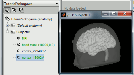
At the end of the process, make sure that the file "cortex_15000V" is selected (downsampled pial surface, which will be used for the source estimation). If it is not, double-click on it to select it as the default cortex surface.
Without the individual MRI
If you do not have access to an individual MR scan of the subject (or if its quality is too low to be processed with FreeSurfer), but if you have digitized the head shape of the subject using a tracking system, you have an alternative: deform one of the Brainstorm templates (Colin27 or ICBM152) to match the shape of the subject's head.
For more information, read the following tutorial: Warping default anatomy
Access the recordings
Link the recordings
- Switch to the "functional data" view.
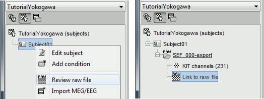
Right-click on the subject folder > Review raw file:
- Select the file format: "MEG/EEG : Yokogawa/KIT"
Select the file: sample_yokogawa/data/SEF_000-export.con
Answer NO when asked to refine the registration using head points. In this dataset, we only have access to the positions of the electrodes and three additional markers on the forehead. The automatic registration doesn't work well in this case, we are going to fix this registration manually.
- A figure is opened to show the current registration MRI/MEG. It is already quite good, but can be improved a bit manually. Close this figure.
- The new file "Link to raw file" lets you access directly the contents of the MEG/EEG recordings
- The channel file "KIT channels" contains the name of the channels and the position of the corresponding sensors.
Prepare the channel file
- The recordings contain signals coming from different types of electrodes:
- 160 MEG channels
- 12 MEG references
- 14 Trigger channels
- 41 EEG channels
- 2 EOG channels: EO1 and EO2
- 1 ECG channel: EKG+
- 1 ground of the EEG amplifier: E
- Not all the types of channels are properly identified in Brainstorm. We need to redefine this manually to get correct groups of sensors.
Right-click on the channel file > Edit channel file:
Channel EO1 (208) and EO2 (209): Change the type to EOG
Channel EKG+ (214): Change the type to ECG
Channel E (231): Change the type to MISC
- Close the figure and accept to save the modifications

Refine the MRI registration
Right-click on the channel file > MRI registration > Edit... (EEG)
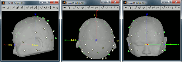
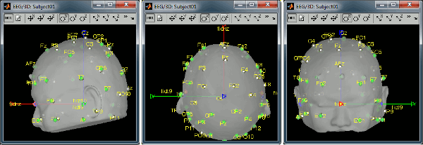
- The white points are the electrodes, the green points are the additional digitized head points. To display the label of the electrodes, click on the [LABEL] button in the toolbar. To see what the other buttons in the toolbar are doing and how to use them, leave your mouse over them for a few seconds and read the description.
Now try to manipulate the position of the EEG+MEG sensors using rotations and translations only (no "resize" or individual electrodes adjustments). The objective is to have all the points close to the surface and the three forehead points inside the little peaks on the surface (due to markers in the MRI).
The rotation+translation are going to be applied both to the EEG and the MEG sensors. After you are done with this solid registration part, you can click on the button "Project electrodes on scalp surface", it will help for the source modeling later. The green points (digitized) stay in place, the white points (electrodes) are now projected on the skin of the subject.
- If you feel like you made it wrong, close the figure and cancel the modifications, then try again. It takes a few trials to get used to this rotation/translation interface.
Click on [OK] when done.
Answer YES to save the modifications.
Answer YES again to apply the solid transformation (rotation+translation) to the MEG sensors.
Before manual registration:
After manual registration:
Read the stimulation information
Right-click on the "Link to raw file" > Trigger > Display time series
- In the Record tab, switch to a column view of the sensors (first button in the toolbar)
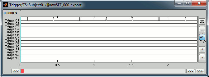
You can see that all the trigger lines are flat except for "Trigger01", which contains the information of the electric stimulation. We are going to read this trigger channel and convert it to a list of events. Close this figure.
- Drag and drop the "Link to raw file" in the Process1 box.
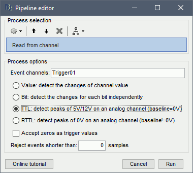
Run the process "Import recordings > Read from channel"
Event channel = Trigger01
Option selected "TTL": detect peaks of 5V/12V on an analog channel
Do not select the option Accept zeros as trigger values
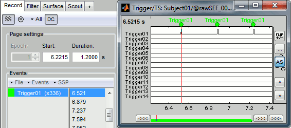
Right-click on the "Link to raw file" > Trigger > Display time series. Check that the peaks of the triggers channel have been correctly identified, then close this figure.
Artifacts: Evaluate the power spectrum
Evaluation
Two of the typical pre-processing steps consist in getting rid of the contamination due to the power lines (50 Hz or 60Hz) and of the frequencies we are not interested in (a low-pass filter to remove the high-frequencies and a high-pass filter to remove the very slow components of the signals). Let's start with the spectral evaluation of this file.
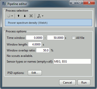
Drag the "Link to raw file" to the Process1 box and run the process "Frequency > Power spectrum density (Welch)". Configure it as illustrated in the following figure:
Time window: [0,50] s, Window length: 4s, Overlap=50%.
Double-click on the new PSD file to display it.
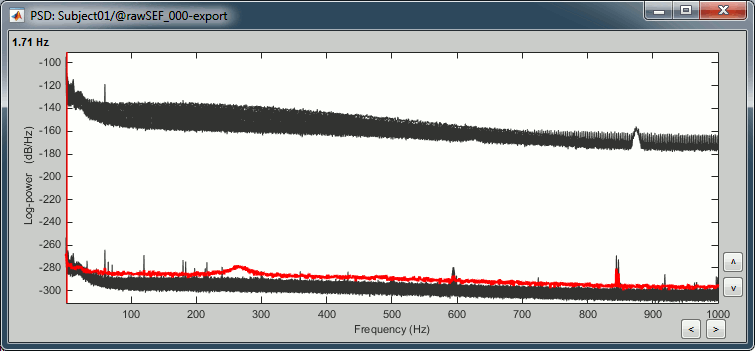
- The lines on the top represent the EEG electrodes, the lines at the bottom the MEG sensors. If you want to get clearer plots, you can calculate separately the spectrum for the two types of sensors separately, by running twice the process "Power spectrum density" , once with sensor types = "MEG" and once with "EEG", instead of running in on both at the same time like we did.
- Observations (below 250Hz):
- Peak around 11Hz: Alpha waves from the subject's brain
Peaks at 60Hz, 120Hz, 180Hz, 240Hz on EEG + MEG:
Electric contamination due to the power lines (60Hz+harmonics)Peaks at 35Hz, 65Hz, 70Hz, 183Hz, 197Hz on MEG only:
Electric noise coming from an unknown sourceMEG sensor LC11 (in red) appears to have a higher level of noise than all the other MEG sensors, we will check this when review the MEG recordings and probably tag it as a bad channel.
Correction
- From the Yokogawa software:
- Users can apply digital filtering to the data before exporting them to Brainstorm. Depending on the data size and degrees of filter parameters, it sometime takes a very long time.
- From Brainstorm:
There is no easy way to process the Yokogawa files at this time using the Brainstorm software. This capability might be added in the future, in which case the procedure would be very similar to the one presented in the basic tutorial ?Detect and remove artifacts.
For short recordings, if the contamination is really bad, there is an alternative option: importing the entire file in Brainstorm and then process it. This approach is illustrated in the EEG/Epilepsy tutorial. This approach requires a very large amount of memory, it is not recommended on MEG recordings as the files tend to be much bigger than EEG-only recordings.
- For now we are going to keep the file as it is. There is no important contamination below 60Hz and we are going to study processes that occur at lower frequencies. When studying evoked responses, the electric noise at 60Hz tends to cancel out and is usually not a problem in the analysis. Note for later that it is however important to consider this electric noise when working on resting state recordings or time-frequency decompositions at higher frequencies.
Artifacts: Heartbeats and eye blinks
Note: The standard pipeline illustrated in the introduction tutorials (first heartbeats and then blinks) does not work well on this dataset. Here we get better results by correcting first the blinks and then the heartbeats.
Detect artifacts and calculate SSP
- Select the "Link to raw file" in the Process1 tab, then create the following analysis pipeline
Process "Events > Detect eye blinks" on channel EO2 (the signal is better than EOG1)
Process "Events > Detect heartbeat" on channel EKG+
Process "Artifacts > SSP: Eye blinks" for MEG
Process "Artifacts > SSP: Eye blinks" for EEG
Process "Artifacts > SSP: Heartbeat" for MEG
Process "Artifacts > SSP: Heartbeat" for EEG
Review the results
- Double-click on the "Link to raw file" to show the MEG sensors
- By default, only the components with a singular value superior to 12% are selected. This is an empirical threshold that does not work all the time. You should always inspect manually all the spatial components you remove from your recordings, to avoid removing any of the data of interest. We are now going to edit the default selections for those four categories.
- Click on [Save] to keep your modifications.
Effect on the artifacts
- If we epoch the recordings based on the blink and cardiac artifacts and average the results, we can evaluate what was the influence of the heartbeats and eye blinks and how much of the artifact is removed for each modality with the SSP projections.
You do not need to do this now, but it is an interesting way of studying these artifacts.
![[ATTACH] [ATTACH]](/moin_static198/brainstorm1/img/attach.png)
Review the recordings
MEG and montages
Right-click on the "Link to raw file" > MEG > Display time series.
- Display the channels in columns (first button in the toolbar of the Record tab).
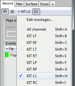
- Check the list of montages available for this file: click on the drop-down menu in the Record tab.
Select the montage "KIT LC"
Load KIT montages
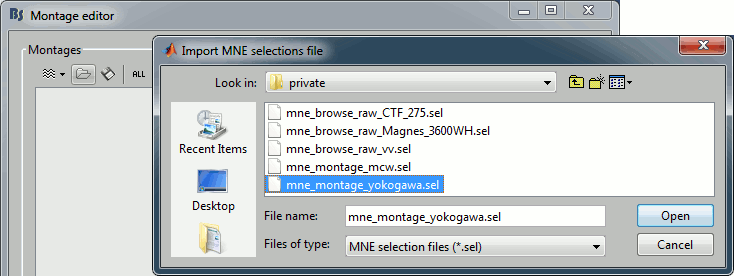
If you don't see all the "KIT..." entries in this list, load them manually:
Click on All > Edit montages...
- Click on the [Load montage] button
- Go to the folder: brainstorm3/toolbox/sensors/private
- Select the file format "MNE selection files (*.sel)"
Select the file mne_montage_yokogawa.sel
Click on save to close the montage editor.
Bad channels (MEG)
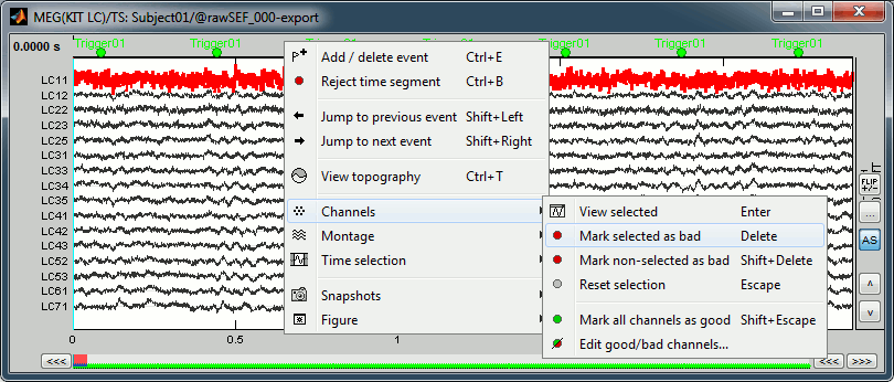
Click on the noisy LC11 sensor to select it (displayed in red)
Press the delete key or right-click in the figure > Channels > Mark selected as bad.
- Close this figure
EEG
Right-click on the "Link to raw file" > EEG > Display time series.
Check the list of available EEG montages.
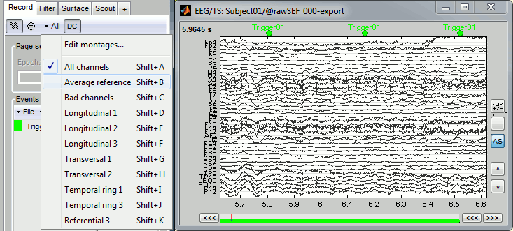
Bad channels (EEG)
In the Record tab, increase the length of the displayed time window to 10s.
You will see that channel TP9 is behaving in a strange way. Select it and mark it as bad.
![[ATTACH] [ATTACH]](/moin_static198/brainstorm1/img/attach.png)
More information
We are not going to detail more in details the interface to review MEG or EEG recordings as it is already done in other specialized tutorials:
For continuous MEG: ?Review continuous recordings and edit markers
For continuous EEG: EEG and epilepsy
For imported files: ?Exploring the recordings
Epoching and averaging
Import recordings
In this experiment, the electric stimulation is sent with a frequency of 2.8Hz, meaning that the inter-stimulus interval is 357ms. We are going to import epochs of 300ms around the stimulation events.
Right-click on the Link to raw file > Import in database:
- Select the entire time definition (0s to 120s, default)
Check "Use events" and select "Trigger01"
Epoch time: [-50, 250] ms
Check "Apply SSP" (make sure that it shows 4 active categories / 4 total projectors)
Check "Remove DC offset" > Time range > [-50, -10] ms
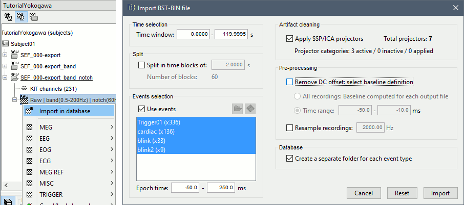
At the end, you are asked whether you want to ignore one epoch that is shorter than the others. This happens because the acquisition of the MEG signals was stopped less than 250ms after the last stimulus trigger was sent. Therefore, the last epoch cannot have the full [-50,250]ms time definition. This shorter epoch would prevent us from averaging all the trials easily. As we already have enough repetitions in this experiment, we can just ignore it.
Answer Yes to this question to discard the last epoch.
Average epochs
- Drag and drop all the Trigger01 trials to the Process1 tab.
Run the process "Average > Average files".
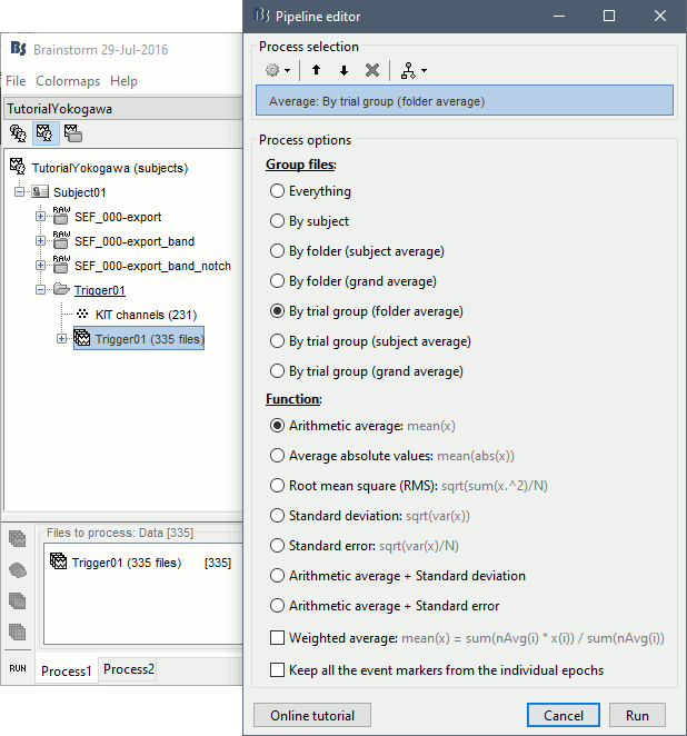
Review the average for the MEG and the EEG.

Source analysis
Head model
We are going to use a realistic head model, this requires to calculate some additional surfaces for the subject, to represent the inner skull and outer skull surface. Go to the "Anatomy" view, right-click on the subject > Generate BEM surfaces.
Use 1922 vertices for each layer (default).
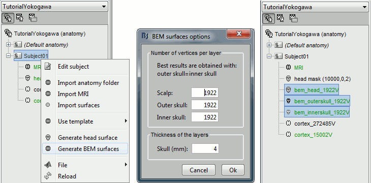
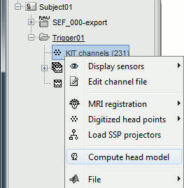
Go back to the "Functional data" view, right-click on the channel file > Compute head model.
Leave all the default options for the head model (cortex surface, MEG=Overlapping, EEG=OpenMEEG). Then leave all the OpenMEEG options to their defaults except for one: select the option "Use adjoint formulation".
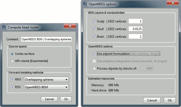
- If the automatic download doesn't work, download OpenMEEG and install it manually (menu Help).
If the OpenMEEG calculation crashes, please refer to the OpenMEEG tutorial.
If you cannot get OpenMEEG to work, or if the results definitely do not make sense, try using a different forward model: "3-shell sphere". It's a spherical model, so it would perform better in the regions of the head that are close to the sphere. See the ?Head model tutorial.
Noise covariance matrix
- We will use the baseline of the single epochs to calculate the noise covariance matrix.
Right-click on the Trigger01 epochs group > Noise covariance > Compute from recordings.
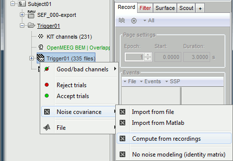
Enter the same baseline interval we used for removing the DC offset: [-50, -10] ms
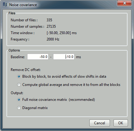
Inverse model
Right-click on the head model > Compute sources.
Select wMNE and MEG. When asked, leave the default list of bad channels (31: channel LC11)
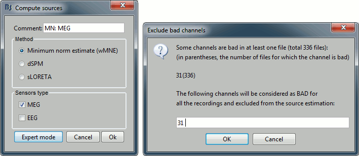
Repeat the same operation for EEG. It is better to study separately the two modalities because the method for combining MEG and EEG are not working well yet.
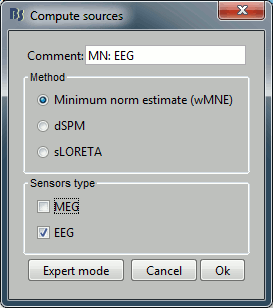
This operation creates a shared inversion kernel and one source link for each block of recordings in the folder. If you are not familiar with those concepts, please refer to the ?Source estimation tutorial.
![[ATTACH] [ATTACH]](/moin_static198/brainstorm1/img/attach.png)
Display the sources for the MEG (top) and the EEG (bottom).
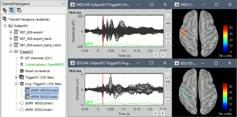
Z-score normalization
- A good way to reveal better the source activity at the cortex level is to calculate a Z-score of the source maps with respect with a quiet baseline. We can use the same baseline as for the calculation of the noise covariance matrix.
- Drag and drop both MEG and EEG average sources in Process1
Run the process: Standardize > Z-score (dynamic), with the baseline [-50,-10]ms
Regions of interest
Create two scouts S1 and S2 to represent the primary and secondary somatosensory cortex of the left hemisphere. Proceed with the method described in the contiunous recordings tutorial:
- Open an average source file (eg. MEG Z-score) and the corresponding recordings
- Go to 20ms, adapt the amplitude threshold and the colormap to see only a focal source
- Create a scout at the center of the activated region
- Grow the scout to about 20 vertices and rename it to "S1"
- Go to 50ms and repeat the same operation for S2. In this specific case, S2 does not appear a clear independent region, as we still see stronger activities in more superior regions of the brain. So pick one activated region around the anatomical location of the secondary somatosensory cortex (at the very bottom of the post-central gyrus). See the picture below.
For more information on the scouts, please refer to the ?scouts tutorial.
Then plot the activity for the different files we calculated.
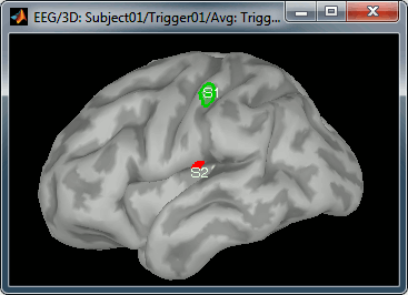
Scripting
The operations described in this tutorial can be reproduced from a Matlab script, available in the Brainstorm distribution: brainstorm3/toolbox/script/tutorial_yokogawa.m
