|
Size: 42125
Comment:
|
Size: 41679
Comment:
|
| Deletions are marked like this. | Additions are marked like this. |
| Line 8: | Line 8: |
| == License == This tutorial dataset (EEG and MRI data) remains proprietary of the Epilepsy Centre, University Hospital Freiburg, Germany. Its use and transfer outside the Brainstorm tutorial, e.g. for research purposes, is prohibited without written consent from the Epilepsy Center in Freiburg. For questions please contact A. Schulze-Bonhage, MD, PhD: andreas.schulze-bonhage@uniklinik-freiburg.de == Presentation of the clinical case == This tutorial dataset was acquired in a patient who suffered from focal epilepsy with focal sensory, dyscognitive and secondarily generalized seizures since the age of eight years. He does not have any typical risk factors for epilepsy. The high resolution 3T epilepsy MRI including postprocessing was found to be normal. FDG-PET of the brain did not show any pathological changes in the glucose metabolism. Non-invasive telemetry revealed left fronto-central sharp waves, polyspikes and bursts of beta band activity (max. amplitude FC1, Cz) especially during sleep. The tutorial dataset was acquired during one night of the non-invasive telemetry recording at the Epilepsy Center Freiburg, Germany. Afterwards the patient underwent invasive EEG to identify the epileptogenic area and to map functionally important cortex. Details about invasive EEG and source localization from invasive EEG in this patient are reported in Dümpelmann, et al. (2011). Subsequently a left frontal tailored resection was performed. The histological analysis revealed a focal cortical dysplasia type IIB according to the classification of Palmini, et al. (2004). The postsurgical outcome is Engel 1A with a follow-up of 5 years. The EEG data distributed here was recorded at 1024Hz, using a Neurofile NT digital video-EEG system with 128 channels and a 16-bit A/D converter. The signal was filtered in the recording system with a high-pass filter with a time constant of 1 second and a low-pass filter with a cutoff frequency of 344 Hz. The spikes were marked with Brainstorm by the epileptologists at the Epilepsy Center in Freiburg. |
<<Include(DatasetEpilepsy, , from="\<\<HTML\(\<!-- START-PAGE --\>\)\>\>", to="\<\<HTML\(\<!-- STOP-SHORT --\>\)\>\>")>> |
| Line 29: | Line 21: |
| Note that the aim of this tutorial is not to train you on how to do spike recognition itself, but rather to illustrate how to manipulate the Brainstorm interface to build a an environment adapted to this task. The formal data reviewing should be done by clinical neurophysiologists or other experienced personnel, with specialized training in separating true epileptic activity from other more normal variants of brain activity. | Note that the aim of this tutorial is not to train you on how to do spike recognition itself, but rather to illustrate how to manipulate the Brainstorm interface to build an environment adapted to this task. The formal data reviewing should be done by clinical neurophysiologists or other experienced personnel, with specialized training in separating true epileptic activity from other more normal variants of brain activity. |
| Line 44: | Line 36: |
| * Go to the [[http://neuroimage.usc.edu/brainstorm3_register/download.php|Download]] page of this website, and download the file: '''sample_epilepsy.zip''' | * Go to the [[http://neuroimage.usc.edu/bst/download.php|Download]] page of this website, and download the file: '''sample_epilepsy.zip''' |
| Line 47: | Line 39: |
| * Select the menu File > Create new protocol. Name it "'''!TutorialEpilepsy'''" and select the options: | * Select the menu File > Create new protocol. Name it "'''TutorialEpilepsy'''" and select the options: |
| Line 52: | Line 44: |
| * Right-click on the !TutorialEpilepsy folder > New subject > '''sepi01''' | * Switch to the "anatomy" view of the protocol. * Right-click on the TutorialEpilepsy folder > '''New subject''' > '''sepi01''' |
| Line 54: | Line 47: |
| * Right-click on the subject node > Import anatomy folder: * Set the file format: "!FreeSurfer folder" |
* Right-click on the subject node > '''Import anatomy folder''': * Set the file format: "FreeSurfer folder" |
| Line 58: | Line 51: |
| * Set the 6 required fiducial points (indicated in MRI coordinates): * NAS: x=135, y=222, z=75 * LPA: x=57, y=118, z=68 * RPA: x=204, y=119, z=76 * AC: x=131, y=145, z=110 * PC: x=130, y=119, z=111 * IH: x=128, y=134, z=170 (anywhere on the midsagittal plane) * At the end of the process, make sure that the file "cortex_15000V" is selected (downsampled pial surface, that will be used for the source estimation). If it is not, double-click on it to select it as the default cortex surface.<<BR>><<BR>> {{attachment:anatomy.gif||height="257",width="442"}} |
* In the MRI Viewer, click on "[[http://neuroimage.usc.edu/brainstorm/Tutorials/ImportAnatomy#MNI_transformation|Click here to compute MNI transformation]]". It compute an affine transformation between the subject space and the MNI ICBM152 space, and sets automatically the anatomical landmarks AC/PC/IH. <<BR>><<BR>> {{attachment:mni_transformation.gif||height="57",width="575"}} * Set the three fiducial points (indicated here in MRI coordinates): * NAS: x=134, y=222, z=74 * LPA: x=58, y=123, z=69 * RPA: x=204, y=120, z=75 * Click on [Save] to validate the modifications and continue with the importation of the anatomy. At the end of the process, make sure that the file "cortex_15000V" is selected (downsampled pial surface, that will be used for the source estimation). If it is not, double-click on it to select it as the default cortex surface.<<BR>><<BR>> {{attachment:anatomy.gif||height="257",width="442"}} |
| Line 68: | Line 59: |
| If you do not have access to an individual MR scan of the subject (or if its quality is too low to be processed with !FreeSurfer), but if you have digitized the head shape of the subject using a tracking system, you have an alternative: deform one of the Brainstorm templates (Colin27 or ICBM152) to match the shape of the subject's head.<<BR>>For more information, read the following tutorial: [[Tutorials/TutWarping|Warping default anatomy]] | If you do not have access to an individual MR scan of the subject (or if its quality is too low to be processed with FreeSurfer), but if you have digitized the head shape of the subject using a tracking system, you have an alternative: deform one of the Brainstorm templates (Colin27 or ICBM152) to match the shape of the subject's head.<<BR>>For more information, read the following tutorial: [[Tutorials/TutWarping|Warping default anatomy]] |
| Line 72: | Line 63: |
| * Switch to the "functional data" view. * Right-click on the subject folder > Review raw file: |
* Switch to the "functional data" view (2nd button, on top of the database explorer). * Right-click on the subject folder > '''Review raw file''': |
| Line 76: | Line 67: |
| * The new file "Link to raw file" lets you access directly the contents of the EEG recordings * The channel file "Deltamed channels" in the (Common files) folder contains the name of the channels, but not their positions. We need to overwrite this file and import manually the positions of the electrodes (either a standard cap or accurate positions digitized with a Polhemus device). |
* The new file "Link to raw file" lets you access directly the contents of the EEG recordings * The channel file "Deltamed channels" in the (Common files) folder contains the name of the channels, but not their positions. We need to overwrite this file and import manually the positions of the electrodes (either a standard cap or accurate positions digitized with a Polhemus device). <<BR>><<BR>> {{attachment:channel_positions.gif||height="205",width="357"}} |
| Line 80: | Line 71: |
| * Right-click on the subject folder > Import channel file: | * Right-click the channel file in ''Common files'' > '''Add EEG positions''' > '''Import from file''': |
| Line 83: | Line 74: |
| * Confirm that you want to overwrite the existing channel file. * This file contains the default electrodes positions from the ASA software (ANT) |
* This file contains the default electrodes positions from the ASA software (ANT). * If you have digitized the position of the electrodes (eg. with a Polhemus device) you have to make sure it contains the position of the anatomical references NAS/LPA/RPA. This is the best way to make sure the electrode cap will be registered automatically with the MRI in Brainstorm. * The channels are matched by name: the position file you import must include the labels of the electrodes and they must be named exactly in the the same way as in your recordings. |
| Line 92: | Line 84: |
| * DELR, DELL, QR, QL: Additional * The file format for the electrodes positions does not describe the type of the channels correctly, therefore all the signals saved in the files are classified as EEG. We need to redefine this manually to get correct groups of sensors, we want to have only real EEG electrodes in the "EEG" category and put everything that we are not going to use a "MISC" category. * Right-click on the channel file > Edit channel file: * Note that the EOG, EMG and ECG channels already have a different type * Select all the other non-EEG channels: SP1, SP2, RS, PHO, DELR, DELL, QR, QL * Right-click in the window > Set channel type: type '''MISC''' * Close the figure and accept to save the modifications {{attachment:channel_type.gif}} |
* DELR, DELL, QR, QL: Not used * It happens commonly that the file format for the electrodes positions does not describe the type of the channels correctly, typically all the signals saved in the files are classified as EEG. We need to redefine this manually to get correct groups of sensors, we want to have only real EEG electrodes in the "EEG" category and put everything that we are not going to use a different category. * Right-click on the channel file > '''Edit channel file''': * Note that the EOG, EMG and ECG channels have their type correctly set. * All the other non-EEG channels were set to "EEG_NO_LOC" when we imported the channel locations: SP1, SP2, RS, PHO, DELR, DELL, QR, QL * In many cases you would have to edit manually the type of some channels: select one channel, click on the type and select something in the drop-down list, or select multiple channels > Right-click in the window > Set channel type. * For this particular study, we can use the channel file as it is configured now, just close the figure. Discard any modification you may have done. {{attachment:channel_type.gif||height="219",width="383"}} |
| Line 105: | Line 97: |
| * Right-click on the channel file > MRI registration > Edit... You will see several buttons across the toolbar; to get the function of a button, hover your mouse for a few seconds over it to reveal the tooltip. * You can click on the "Label" button in the toolbar to show the electrode names. The default positions are already quite good, and the head shape is correct; only limited manual registration will be required in the next few steps. |
* Right-click on the channel file > '''MRI registration''' > '''Edit...''' You will see several buttons across the toolbar; to get the function of a button, hover your mouse for a few seconds over it to reveal the tooltip. * Click on the [Label] button in the toolbar to show the names''' '''of the electrodes. The default positions are already quite good, and the head shape is correct; only limited manual registration will be required in the next few steps. |
| Line 119: | Line 111: |
| * Right-click on the "Link to raw file" > EEG > Display time series. * In the tab Record, menu File > Add events from files... * Select file format "Array of times" (We are importinga a text file containing the timing of the markers) |
* Right-click on the "Link to raw file" > EEG > '''Display time series''' (or simply double-click on the file). * In the tab Record, menu File > '''Add events from files'''... * Select format '''Array of times''' (importing a a text file containing the timing of the markers) |
| Line 124: | Line 116: |
| * Note that a new category SPIKE is visible in the events list, containing 58 markers * Close the viewer and agree to save the modifications ==== Display the recordings in one montage ==== * For basic information on how to manipulate the montages in Brainstorm: [[http://%20neuroimage.usc.edu/brainstorm/Tutorials/TutExploreRecodings#Montages|read this tutorial]]. |
* Note that a new category SPIKE is visible in the events list, containing 58 markers. <<BR>><<BR>> {{attachment:events_import.gif}} * Close the viewer and agree to save the modifications. ==== Display the recordings ==== |
| Line 132: | Line 123: |
| * Select the "Average reference" in the drop-down list. This menu allows you to set a predefined montages to linearly re-arranging the waveforms. Note the keyboard shortcuts in the menus. * In the Record tab, change the default duration that is reviewed to '''10s'''. * In the figure, click on the '''[Flip +/-]''' button to have the negative values pointing up (convention used by most neurologists) |
* Select the "Average reference" in the drop-down list. This menu allows you to set a predefined montages to linearly re-arranging the waveforms. Note the keyboard shortcuts in the menus. <<BR>><<BR>> {{attachment:review_avgref.gif||height="129",width="188"}} * In the Record tab, change the default duration that is reviewed to '''10s'''. {{attachment:review_duration.gif||height="66",width="198"}} * In the figure, click on the '''[Flip +/-]''' button to have the negative values pointing up (convention used by most neurologists). <<BR>><<BR>> {{attachment:review_flip.gif||height="166",width="360"}} |
| Line 136: | Line 127: |
| * Right-click on "Link to raw file" again > EEG > '''2D Sensor cap ''' | * Right-click on "Link to raw file" again > EEG > '''2D Sensor cap''' |
| Line 138: | Line 129: |
| * Open the '''ECG '''and '''EOG '''traces as well, to avoid confusing spikes with cardiac or ocular artifacts:<<BR>> | * Open the '''ECG '''and '''EOG '''traces as well, to avoid confusing spikes with cardiac or ocular artifacts: |
| Line 144: | Line 135: |
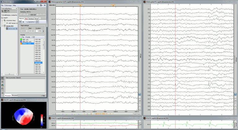
| * Review a few existing SPIKE events, to get the feeling of how this reviewing environment works. {{attachment:reviewall.gif}} |
* Review a few existing SPIKE events, to get the feeling of how this reviewing environment works.<<BR>><<BR>> {{attachment:reviewall.gif||height="322",width="594"}} |
| Line 152: | Line 141: |
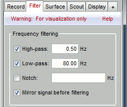
| * Low-pass filter: '''70 Hz'''<<BR>><<BR>> {{attachment:filters.gif||height="175",width="205"}} | * Low-pass filter: '''80 Hz'''<<BR>><<BR>> {{attachment:filters.gif||height="165",width="196"}} |
| Line 157: | Line 146: |
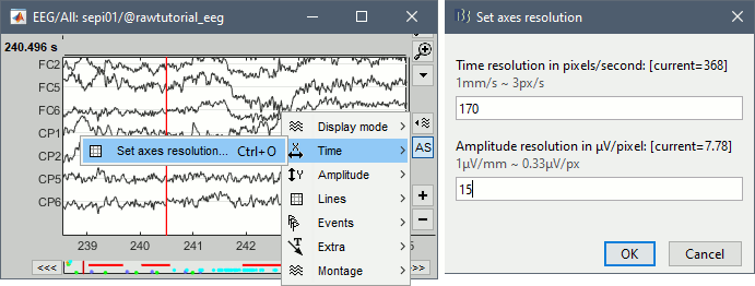
| In the Brainstorm interface, this resolution is usually set implicitly: you can set the size of the window, the duration or recordings reviewed at once (text box "duration" in tab Record) and the maximum amplitude to show in the figure (buttons [...] and [AS] on the right of the time series figure). From there, you can also zoom in time ([<], [>], mouse wheel) or amplitude (['''^'''], [v], Shift+mouse wheel). Those parameters are convenient to explore the recordings interactively but don't allow us to have reproducible displays with constant time and amplitude resolutions. To set the figure resolution explicitly: right-click on the figure > Figure > Set axes resolution. Note that this interface does not store the input values, it just modifies the other parameters (figure size, time window, max amplitude) to fit the resolution objectives. Then if you modify those parameters (resize the figure, leave the button [AS] selected and scroll in time, etc) the resolution is lost, you have to set it again manually. |
In the Brainstorm interface, this resolution is usually set implicitly: you can set the size of the window, the duration or recordings reviewed at once (text box "duration" in tab Record) and the maximum amplitude to show in the figure (buttons [...] and [AS] on the right of the time series figure). From there, you can also zoom in time ([<], [>], mouse wheel) or amplitude (['''^'''], [v], Shift+mouse wheel). These parameters are convenient to explore the recordings interactively but don't allow us to have reproducible displays with constant time and amplitude resolutions. To set the figure resolution explicitly: right-click on the figure > Figure > Set axes resolution. Note that this interface does not store the input values, it just modifies the other parameters (figure size, time window, max amplitude) to fit the resolution objectives. If you modify these parameters (resize the figure, leave the button [AS] selected and scroll in time, etc) the resolution is lost, you have to set it again manually. In particular, make sure you '''disable the auto-scaling''' ([AS] button in the time series figure) if you want to preserve the aspect ratio while you scroll through the data. |
| Line 167: | Line 156: |
| This preparation of the reviewing environment requires a large number of operations, and would become quickly annoying if you have to repeat it every time you open a file. This is a good time to use the menu "User setups" to save this window configuration, to reload it in one click later. In the menu "Window layout", at the top-right of the Brainstorm window, select User setup > New setup. Enter a name of your choice for this particular window arrangement. | This preparation of the reviewing environment requires a large number of operations, and would become quickly annoying if you have to repeat it every time you open a file. This is a good time to use the menu "User setups" to save this window configuration, so that you can reload it in one click later. In the menu "Window layout", at the top-right of the Brainstorm window, select User setup > New setup. Enter a name of your choice for this particular window arrangement. |
| Line 183: | Line 172: |
| * If you don't see the "Longitudinal 3" menu, it is probably because you have using Brainstorm before those predefined montages were made available in the software distribution. To add them manually: | * If you don't see the "Longitudinal 3" menu, it is probably because you have using Brainstorm before these predefined montages were made available in the software distribution. To add them manually: |
| Line 191: | Line 180: |
| {{attachment:reviewall2.gif}} | {{attachment:reviewall2.gif||height="372",width="678"}} |
| Line 202: | Line 191: |
| * Scroll through the recordings using the [<<<] and [>>>] buttons or shortcuts such as F3 or F4 (complete list and descriptions available when you leave your mouse over those buttons). * You can adjust the gain of the electrodes to observe better an event with the buttons ['''^'''] and [v] or the shortcut [Shift+mouse wheel]. |
* Scroll through the recordings using the [<<<] and [>>>] buttons or shortcuts such as F3 or F4 (complete list and descriptions available when you leave your mouse over these buttons). * You can adjust the gain of the electrodes to observe better an event with the buttons ['''^'''] and [v], with the keyboard (+/-) or the mouse ([Shift+mouse wheel] or [Right-click+move up/down]). |
| Line 208: | Line 197: |
| * More information on the data viewer, see tutorial: [[Tutorials/TutRawViewer|Review continuous recordings]]. | * More information on the data viewer, see tutorial: [[Tutorials/ReviewRaw|Review continuous recordings]]. |
| Line 211: | Line 200: |
| ==== Average reference ==== | |
| Line 216: | Line 206: |
| * The sharp drop we observe at 50Hz on all the electrodes indicates that a notch filter was already applied to the data, we do not need to remove the power line contamination again. If we had to, we would run the process "Pre-processing > Sinusoid removal (notch)" as explained in the tutorial [[Tutorials/TutRawSsp|Detect and remove artifacts]]. ==== High-pass filter ==== We would like to apply a 0.5Hz high-pass filter to the entire file in order to get rid of the long amplitude fluctuations (longer than 2s). With some MEG file formats, Brainstorm supports the creation of new filtered files in native formats, which means that you can drag and grop directly the "Link to raw file" to the Process1 tab and run the band-pass filter process. Unfortunately, this is currently not supported for the file format we are currently working on (Deltamed Coherence-Neurofile). There is an alternative option which consists in importing the entire continuous file in the database in one single block, then run the filter on it. This approach works is possible only on rather small files (4 * file size < memory on the computer). Here the file size is less than 80 Mb, so it can be easily processed this way. * Right-click on the "Link to raw file" > Import in database. * Uncheck all the options and leave the default "Time window" option. <<BR>><<BR>> {{attachment:import_all.gif||height="295",width="490"}} * Click on Import, it creates an integral copy of the file in the database. Do NOT try to review it: for imported file, the partial loading and the scrolling in time are disabled and it would take a lot of time to display the waveforms for the entire file. It could event result in a crash of Brainstorm or Matlab. * Drag this new file "Raw (0s,3600s)" to the Process1 |
* This frequency spectrum does not show any particular peak at 50/60Hz, there is no notch filter to apply on these recordings. If we had to, we would run the process "Pre-processing > Notch filter" as explained in the tutorial [[Tutorials/ArtifactsFilter|Detect and remove artifacts]]. ==== Band-pass filter ==== We would like to apply a band-pass filter to keep only the frequencies between 0.5Hz an 80Hz. The high-pass filter at 0.5Hz will rid of the slow amplitude fluctuations (longer than 2s). * Leave the "Link to raw file" selected in the Process1 list. |
| Line 228: | Line 213: |
| * Lower cutoff frequency: '''0.5Hz''' (high-pass filter at 0.5Hz) * Upper cutoff frequency: '''0Hz''' (no low-pass filter) |
* Lower cutoff frequency: '''0.5 Hz''' (high-pass filter) * Upper cutoff frequency: '''80 Hz''' (low-pass filter) |
| Line 231: | Line 216: |
| * Sensor types: '''EMPTY '''(to process all the signals) * Overwrite: '''On''' (we don't need to keep the original copy)<<BR>><<BR>> {{attachment:bandpass.gif||height="284",width="494"}} |
* Sensor types: '''EMPTY '''(to process all the signals)<<BR>><<BR>> {{attachment:bandpass.gif||height="281",width="295"}} * Note that this new continuous files is saved in your Brainstorm database, while your original file is saved in a separate folder (sample_epilepsy). If you delete the link to the original file with the database explorer, it would not delete the actual file. If you delete the link to the filtered file, it would delete the file itself. * Drag this new file "Raw | band(0.5-80Hz)" to the Process1 list. * Run again the process "Frequency > Power spectrum density (Welch)", with same options as before. * Double-click on the new PSD file to display the spectrum of the filtered file.<<BR>><<BR>> {{attachment:psd3.gif||height="190",width="489"}} |
| Line 237: | Line 227: |
| * Right-click on the imported and filtered file '''"Raw (0s,3600s) | high(0.5Hz)"''' > Import in database<<BR>><<BR>> {{attachment:import_menu.gif||height="177",width="242"}} | * Right-click on the imported and filtered file '''"Raw (0s,3600s) | high(0.5Hz)"''' > Import in database<<BR>><<BR>> {{attachment:import_menu.gif||height="150",width="226"}} |
| Line 241: | Line 231: |
| * You should see a new folder "SPIKE" containing 58 epochs in your database.<<BR>><<BR>> {{attachment:import_after.gif||height="242",width="219"}} | * You should see a new folder "SPIKE" containing 58 epochs in your database.<<BR>><<BR>> {{attachment:import_after.gif||height="166",width="228"}} |
| Line 245: | Line 235: |
| * Run the process "Average > Average files", with the following options:<<BR>><<BR>> {{attachment:average1.gif||height="473",width="456"}} | * Run the process "Average > Average files", with the following options:<<BR>><<BR>> {{attachment:average1.gif||height="405",width="408"}} |
| Line 247: | Line 237: |
| * Go to the Filter tab to __'''disable all the visualization filters'''__: those filters are not working well on short signals, the high-pass filter at 0.5Hz can introduce errors in the display of the average. * Open a "2D sensor cap" view on the same file, or simply press [Ctrl+T] from the time series figure.<<BR>><<BR>> {{attachment:average_view.gif||height="238",width="438"}} * To have all the figures re-arrange themselves automatically again, select "Weighted" or "Tiled" in the "Window layout" menu (top-right corner). |
* Go to the Filter tab to __'''disable all the visualization filters'''__: these filters are not working well on short signals, the high-pass filter at 0.5Hz can introduce errors in the display of the average. * Open a "2D sensor cap" view on the same file, or simply press [Ctrl+T] from the time series figure.<<BR>><<BR>> {{attachment:average_view.gif||height="205",width="409"}} * To have all the figures automatically re-arrange themselves again, select "Weighted" or "Tiled" in the "Window layout" menu (top-right corner). |
| Line 259: | Line 249: |
| * Use '''1922 vertices '''for each layer (default). Three new surface files are created at the end of the process.<<BR>><<BR>> {{attachment:bem1.gif||height="273",width="196"}} {{attachment:bem2.gif||height="240",width="184"}} {{attachment:bem3.gif||height="272",width="157"}} | * Use '''1922 vertices '''for each layer (default). Three new surface files are created at the end:<<BR>><<BR>> {{attachment:bem1.gif||height="273",width="196"}} {{attachment:bem2.gif||height="240",width="184"}} {{attachment:bem3.gif||height="272",width="157"}} |
| Line 262: | Line 252: |
| * If you can't download OpenMEEG automatically, download and install it manually (menu Help) | * If the automatic download doesn't work, download and install OpenMEEG manually (menu Help) |
| Line 265: | Line 255: |
| * If you cannot get OpenMEEG to work, or if the results definitely do not make sense, try using a different forward model: "'''3-shell sphere'''". It's a spherical model, so it would perform better in the regions of the head that are close to the sphere. See the [[Tutorials/TutHeadModel|Head model tutorial]]. | * If you cannot get OpenMEEG to work, or if the results definitely do not make sense, try using a different forward model: "'''3-shell sphere'''". It's a spherical model, so it would perform better in the regions of the head that are close to the sphere. See the [[Tutorials/HeadModel|Head model tutorial]]. |
| Line 268: | Line 258: |
| * For minimum norm inverse models, we need to estimate first the level of noise at the level of the sensors. Defining what can be considered as "noise" in the middle of continuous brain recordings is a difficult question, discussed in the [[Tutorials/TutNoiseCov|Noise covariance tutorial]]. | * For minimum norm inverse models, we need to estimate first the level of noise at the level of the sensors. Defining what can be considered as "noise" in the middle of continuous brain recordings is a difficult question, discussed in the [[Tutorials/NoiseCovariance|Noise covariance tutorial]]. |
| Line 277: | Line 267: |
| * This operation creates a shared inversion kernel in the folder (Common files) and one source link for each block of recordings in subject sepi01. If you are not familiar with those concepts, please refer to the [[Tutorials/TutSourceEstimation|Source estimation tutorial]]. <<BR>><<BR>> {{attachment:inverse2.gif||height="201",width="210"}} * Double-click on the sources file for the average to open it. Configure its display: surface smoothing, amplitude threshold, colormap. For a reminder on how to manipulate the colormaps, see the tutorial [[http://neuroimage.usc.edu/brainstorm/Tutorials/TutExploreRecodings#Colormap_configuration|Explore recordings]]. |
* This operation creates a shared inversion kernel in the folder (Common files) and one source link for each block of recordings in subject sepi01. If you are not familiar with these concepts, please refer to the [[Tutorials/SourceEstimation|Source estimation tutorial]]. <<BR>><<BR>> {{attachment:inverse2.gif||height="201",width="210"}} * Double-click on the sources file for the average to open it. Configure its display: surface smoothing, amplitude threshold, colormap. For a reminder on how to manipulate the colormaps, see the tutorial [[Tutorials/Colormaps|Colormaps]]. |
| Line 285: | Line 275: |
| * The inverse solutions that you calculated are all shared for all the recordings in this subject, so you can go back to your individual epochs, or even the continuous file, and look at the source maps for those files. | * The inverse solutions that you calculated are all shared for all the recordings in this subject, so you can go back to your individual epochs, or even the continuous file, and look at the source maps for these files. |
| Line 291: | Line 281: |
| * Plot the overlayed time series for those scouts. Try with the scout functions MEAN and MAX. | * Plot the overlayed time series for these scouts. Try with the scout functions MEAN and MAX. |
| Line 293: | Line 283: |
| * If you need a reminder on how to manipulate scouts: see the [[Tutorials/TutScouts|Scouts tutorial]]<<BR>><<BR>> {{attachment:scouts1.gif||height="189",width="478"}} | * If you need a reminder on how to manipulate scouts: see the [[Tutorials/Scouts|Scouts tutorial]]<<BR>><<BR>> {{attachment:scouts1.gif||height="189",width="478"}} |
| Line 327: | Line 317: |
| Coming soon... | This section is on a different page: [[Tutorials/EpilepsyBest|Link]] |
| Line 337: | Line 327: |
| Benar CG, Grova C, Kobayashi E, Bagshaw AP, Aghakhani Y, Dubeau F, Gotman J (2006)<<BR>>[[http://www.ncbi.nlm.nih.gov/pubmed/16413798|EEG–fMRI of epileptic spikes: Concordance with EEG source localization and intracranial EEG]]<<BR>>!NeuroImage, 30:1161-1170. | Benar CG, Grova C, Kobayashi E, Bagshaw AP, Aghakhani Y, Dubeau F, Gotman J (2006)<<BR>>[[http://www.ncbi.nlm.nih.gov/pubmed/16413798|EEG–fMRI of epileptic spikes: Concordance with EEG source localization and intracranial EEG]]<<BR>>NeuroImage, 30:1161-1170. ==== Forum posts ==== * EEG reference: http://neuroimage.usc.edu/forums/showthread.php?1525#post6718 |
| Line 344: | Line 337: |
| * Folder to import: '''sample_epilepsy/anatomy''' (format = !FreeSurfer) | * Folder to import: '''sample_epilepsy/anatomy''' (format = FreeSurfer) |
| Line 346: | Line 339: |
| * Because of the selection of those points, it usally to run this first step in interactive mode...MISC | * Because of the selection of these points, it is usally better to run this first step in interactive mode. |
| Line 358: | Line 351: |
| * Import recordings > Events: Import from file | * Events > Import from file |
| Line 413: | Line 406: |
| ==== Graphic edition ==== {{attachment:script.gif}} ==== Generate Matlab script ==== This list of processes can be converted automatically to a Matlab script.<<BR>>See the results on the page: [[Tutorials/EpilepsyScript|EEG and epilepsy: Script]]. == Feedback == <<EmbedContent(http://neuroimage.usc.edu/brainstorm3_register/get_feedback.php?Tutorials/Epilepsy)>> |
The following script from the Brainstorm distribution reproduces the analysis presented in this tutorial page: '''brainstorm3/toolbox/script/tutorial_epilepsy''''''.m''' <<HTML(<div style="border:1px solid black; background-color:#EEEEFF; width:720px; height:500px; overflow:scroll; padding:10px; font-family: Consolas,Menlo,Monaco,Lucida Console,Liberation Mono,DejaVu Sans Mono,Bitstream Vera Sans Mono,Courier New,monospace,sans-serif; font-size: 13px; white-space: pre;">)>><<EmbedContent("http://neuroimage.usc.edu/bst/viewcode.php?f=tutorial_epilepsy.m")>><<HTML(</div >)>> <<EmbedContent(http://neuroimage.usc.edu/bst/get_feedback.php?Tutorials/Epilepsy)>> |
EEG and epilepsy
Authors: Francois Tadel, Elizabeth Bock, John C. Mosher.
This tutorial introduces some concepts that are specific to the management of EEG recordings in the Brainstorm environment. It also describes a standard pipeline for analyzing epilepsy recordings. It is based on a clinical case from the Epilepsy Center at the University Hospital of Freiburg, Germany. The anonymized dataset can be downloaded directly from the Brainstorm download page.
Contents
- Dataset description
- Overview of the data processing
- Download and installation
- Import the anatomy
- Access the recordings
- Review EEG recordings
- Mark spikes
- Pre-process recordings
- Epoching and averaging
- Source analysis: Cortically constrained
- Source analysis: Full head volume
- Moving dipoles
- MEM inverse solution
- Discussion
- Scripting
Dataset description
License
This tutorial dataset (EEG and MRI data) remains proprietary of the Epilepsy Centre, University Hospital Freiburg, Germany. Its use and transfer outside the Brainstorm tutorial, e.g. for research purposes, is prohibited without written consent from the Epilepsy Centre in Freiburg. For questions please contact A. Schulze-Bonhage, MD, PhD: andreas.schulze-bonhage@uniklinik-freiburg.de
Clinical description
This tutorial dataset was acquired in a patient who suffered from focal epilepsy with focal sensory, dyscognitive and secondarily generalized seizures since the age of eight years. He does not have any typical risk factors for epilepsy. The high resolution 3T epilepsy MRI including postprocessing was found to be normal. FDG-PET of the brain did not show any pathological changes in the glucose metabolism. Non-invasive telemetry revealed left fronto-central sharp waves, polyspikes and bursts of beta band activity (max. amplitude FC1, Cz) especially during sleep. The tutorial dataset was acquired during one night of the non-invasive telemetry recording at the Epilepsy Center Freiburg, Germany.
Afterwards the patient underwent invasive EEG to identify the epileptogenic area and to map functionally important cortex. Details about invasive EEG and source localization from invasive EEG in this patient are reported in Dümpelmann, et al. (2011). Subsequently a left frontal tailored resection was performed. The histological analysis revealed a focal cortical dysplasia type IIB according to the classification of Palmini, et al. (2004). The postsurgical outcome is Engel 1A with a follow-up of 5 years.
The EEG data distributed here was recorded at 256Hz, using a Neurofile NT digital video-EEG system with 128 channels and a 16-bit A/D converter. The signal was filtered in the recording system with a high-pass filter with a time constant of 1 second (cutoff frequency ~ 0.16Hz) and a low-pass filter with a cutoff frequency of 344 Hz. The spikes were marked with Brainstorm by the epileptologists at the Epilepsy Center in Freiburg.
Overview of the data processing
The proper identification of epileptiform discharges ("spikes") is a complicated topic beyond the scope of this tutorial. Residents in Neurology train intensively on how to identify true interictal and ictal discharges, particularly as distinct from so-called "normal variants" that can be abundant. Sleep and drowsy states of the brain can generate "vertex waves," "K-complexes," "positive occipital sharp transients of sleep" (POSTS), and "wickets," to name a few variants, none of which are epileptic. A good overview of terminology and application can be found, for example, on the Medscape website, Epileptiform Discharges.
With this caveat, we nonetheless give an overview of the processing approach. Although automation has been proposed for decades, "spike hunting" is often done by manual inspection of the recorded EEG waveforms (whether scalp, subdural, or depths). The classic scalp sensor arrangement is the International 10-20 System (Wikipedia Site, Bioelectromagnetism Book, Chapter 13.3) arranged at 10 percent and 20 percent distances about the circumference of the head. Each of these 21 electrodes is acquired with respect to some reference (as all potentials must be). In reviewing the recordings, however, several "montages" are traditionally recommended that digitally "re-reference" the original recordings into new linear combinations of electrodes.
A classic montage is the "double banana" (Google Search) which emphasizes local changes in the scalp EEG by forming sequential bipolar pairs, such as "Fp1-F3", "F3-C3." Because F3 is found twice in this montage and of opposite sign, then an epileptic spike centered under F3 will appear as a reversed polarity in these two channels, a visual cue the trained epileptologist seeks when rapidly scanning through hours of recordings. This montage is more formally known as "LB-18.3" or "Longitudinal Bipolar 3" in the nomenclature of the American Clinical Neurophysiology Society (ACNS) Guidelines (see References Below).
ACNS guidelines suggest using both "longitudinal" and "transversal" bipolar montages to survey your data. For temporal epilepsy cases, you may also add a "temporal ring" montage. European neurologists often prefer to review the recordings using an average reference montage. Brainstorm provides several variations of all these montages, allows the users full flexibility in creating their own, and can run different montages simultaneously in multiple windows.
The user has to step along through the data, look for abnormal brain activity, then use Brainstorm's event markers to tag suspect intervals. With the suspected events marked and saved, the user can return later to perform source analyses on these intervals. With this brief overview, we detail below an exercise with the sample epilepsy data.
Note that the aim of this tutorial is not to train you on how to do spike recognition itself, but rather to illustrate how to manipulate the Brainstorm interface to build an environment adapted to this task. The formal data reviewing should be done by clinical neurophysiologists or other experienced personnel, with specialized training in separating true epileptic activity from other more normal variants of brain activity.
References
Dümpelmann M, Ball T, Schulze-Bonhage A (2011)
sLORETA allows reliable distributed source reconstruction based on subdural strip and grid recordings. Human Brain Mapping.
Palmini A, Najm I, Avanzini G, Babb T, Guerrini R, Foldvary-Schaefer N, Jackson G, Luders HO, Prayson R, Spreafico R, Vinters HV (2004) Terminology and classification of the cortical dysplasias.
Neurology, 62:S2-8.
Standard montages recommended by the American Clinical Neurophysiology Society:
Download and installation
Requirements: You have already followed all the introduction tutorials and you have a working copy of Brainstorm installed on your computer.
Go to the Download page of this website, and download the file: sample_epilepsy.zip
Unzip it in a folder that is not in any of the Brainstorm folders (program folder or database folder)
- Start Brainstorm (Matlab scripts or stand-alone version)
Select the menu File > Create new protocol. Name it "TutorialEpilepsy" and select the options:
"No, use individual anatomy",
"Yes, use one channel file per subject".
Import the anatomy
- Switch to the "anatomy" view of the protocol.
Right-click on the TutorialEpilepsy folder > New subject > sepi01
- Leave the default options you set for the protocol
Right-click on the subject node > Import anatomy folder:
Set the file format: "FreeSurfer folder"
Select the folder: sample_epilepsy/anatomy
- Number of vertices of the cortex surface: 15000 (default value)
In the MRI Viewer, click on "Click here to compute MNI transformation". It compute an affine transformation between the subject space and the MNI ICBM152 space, and sets automatically the anatomical landmarks AC/PC/IH.

- Set the three fiducial points (indicated here in MRI coordinates):
- NAS: x=134, y=222, z=74
- LPA: x=58, y=123, z=69
- RPA: x=204, y=120, z=75
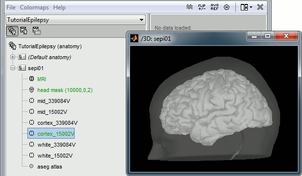
Click on [Save] to validate the modifications and continue with the importation of the anatomy. At the end of the process, make sure that the file "cortex_15000V" is selected (downsampled pial surface, that will be used for the source estimation). If it is not, double-click on it to select it as the default cortex surface.
Without the individual MRI
If you do not have access to an individual MR scan of the subject (or if its quality is too low to be processed with FreeSurfer), but if you have digitized the head shape of the subject using a tracking system, you have an alternative: deform one of the Brainstorm templates (Colin27 or ICBM152) to match the shape of the subject's head.
For more information, read the following tutorial: Warping default anatomy
Access the recordings
Link the recordings
- Switch to the "functional data" view (2nd button, on top of the database explorer).
Right-click on the subject folder > Review raw file:
- Select the file format: "EEG: Deltamed Coherence-Neurofile(*.bin)"
Select the file: sample_epilepsy/data/tutorial_eeg.bin
- The new file "Link to raw file" lets you access directly the contents of the EEG recordings
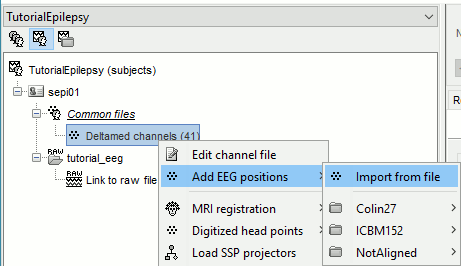
The channel file "Deltamed channels" in the (Common files) folder contains the name of the channels, but not their positions. We need to overwrite this file and import manually the positions of the electrodes (either a standard cap or accurate positions digitized with a Polhemus device).
Prepare the channel file
Right-click the channel file in Common files > Add EEG positions > Import from file:
- Select the file format: "EEG: ANT Xensor (*.elc)"
Select the file: sample_epilepsy/data/tutorial_electrodes.elc
- This file contains the default electrodes positions from the ASA software (ANT).
- If you have digitized the position of the electrodes (eg. with a Polhemus device) you have to make sure it contains the position of the anatomical references NAS/LPA/RPA. This is the best way to make sure the electrode cap will be registered automatically with the MRI in Brainstorm.
- The channels are matched by name: the position file you import must include the labels of the electrodes and they must be named exactly in the the same way as in your recordings.
- The recordings contain signals coming from different types of electrodes:
- 29 EEG electrodes
- EOG1, EOG2: Electrooculograms
- EMG, ECG: Electromyogram and electrocardiogram
- SP1, SP2: Sphenoidal electrodes
- RS: Electrode on the right shoulder
- PHO: Photo stimulation channel
- DELR, DELL, QR, QL: Not used
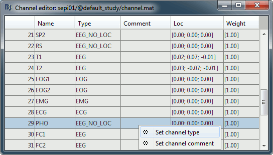
- It happens commonly that the file format for the electrodes positions does not describe the type of the channels correctly, typically all the signals saved in the files are classified as EEG. We need to redefine this manually to get correct groups of sensors, we want to have only real EEG electrodes in the "EEG" category and put everything that we are not going to use a different category.
Right-click on the channel file > Edit channel file:
- Note that the EOG, EMG and ECG channels have their type correctly set.
- All the other non-EEG channels were set to "EEG_NO_LOC" when we imported the channel locations: SP1, SP2, RS, PHO, DELR, DELL, QR, QL
In many cases you would have to edit manually the type of some channels: select one channel, click on the type and select something in the drop-down list, or select multiple channels > Right-click in the window > Set channel type.
- For this particular study, we can use the channel file as it is configured now, just close the figure. Discard any modification you may have done.
Register electrodes with MRI
- The channel file we imported contains generic electrodes positions; hence, it cannot be fully aligned with the head surface coming from the MRI. We need to register manually these electrodes positions with the subject anatomy.
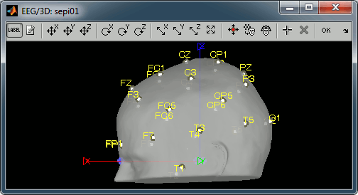
Right-click on the channel file > MRI registration > Edit... You will see several buttons across the toolbar; to get the function of a button, hover your mouse for a few seconds over it to reveal the tooltip.
Click on the [Label] button in the toolbar to show the names of the electrodes. The default positions are already quite good, and the head shape is correct; only limited manual registration will be required in the next few steps.
- Click on the button "Refine registration using head points" to find a better registration between the head shape defined by the electrodes and the head surface coming from the MRI.
- Click on the button "Project electrodes on scalp surface", to ensure all the electrodes touch the skin surface.
Click on "OK" and agree to save the modifications.
Review EEG recordings
Import the spike markers
Some spikes were marked by the epileptologists at the Epilepsy Center in Freiburg with Brainstorm and saved in an external text file. We are going to import this file manually.
Right-click on the "Link to raw file" > EEG > Display time series (or simply double-click on the file).
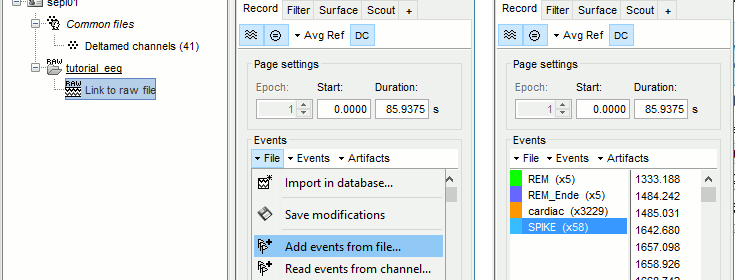
In the tab Record, menu File > Add events from files...
Select format Array of times (importing a a text file containing the timing of the markers)
Select file sample_epilepsy/data/tutorial_spikes.txt
When prompted, enter the event name "SPIKE"
Note that a new category SPIKE is visible in the events list, containing 58 markers.
- Close the viewer and agree to save the modifications.
Display the recordings
Open a time series figure with the "Average reference" montage
Right-click on the "Link to raw file" > EEG > Display time series.
- In the Record tab, select the first button in the toolbar (Display mode for time series) to view the signals in columns.
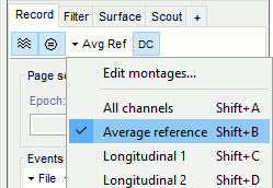
Select the "Average reference" in the drop-down list. This menu allows you to set a predefined montages to linearly re-arranging the waveforms. Note the keyboard shortcuts in the menus.
In the Record tab, change the default duration that is reviewed to 10s.

In the figure, click on the [Flip +/-] button to have the negative values pointing up (convention used by most neurologists).

Open a 2D Sensor cap map of the EEG sensor values as well:
Right-click on "Link to raw file" again > EEG > 2D Sensor cap
In the Record tab, set the Montage to this view to "Average reference"
Open the ECG and EOG traces as well, to avoid confusing spikes with cardiac or ocular artifacts:
Right-click on the Link to raw file > ECG > Display time series
Right-click on the Link to raw file > EOG > Display time series
- The ECG is almost mandatory. The EOG is optional: it can be helpful for beginners but an experienced reviewer will easily recognize the eye movements directly in the EEG data.
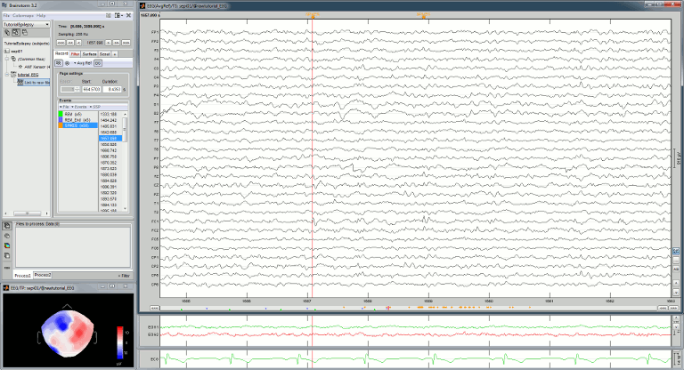
Re-arrange the figures in a convenient way, for example as illustrated below, and disable the automatic positioning of the figures you the figure arrangement doesn't get lost when you open a new figure (Window layout menu at the top-right of the Brainstorm figure > None)
- Having a lot of windows open may slow down significantly the display because each time you change the current time, all the figures have to be updated. A lot of space is also wasted on the screen due to window frames. The number of windows to open has to be a balance between the amount of information to display and the ease of use.
Review a few existing SPIKE events, to get the feeling of how this reviewing environment works.
Frequency filters
Go to the Filter tab to enable some display frequency filters. General recommendations are:
High-pass filter: 0.5 Hz
Low-pass filter: 80 Hz
Time and amplitude resolution
The resolutions of the time and amplitude axes has a lot of importance for the visual detection of epileptic spikes. The shapes we are looking for are altered by the horizontal and vertical scaling. The distance unit on a screen is the pixel, we can set how much time is represented by one pixel horizontally and how much amplitude is represented by one pixel vertically.
In the Brainstorm interface, this resolution is usually set implicitly: you can set the size of the window, the duration or recordings reviewed at once (text box "duration" in tab Record) and the maximum amplitude to show in the figure (buttons [...] and [AS] on the right of the time series figure). From there, you can also zoom in time ([<], [>], mouse wheel) or amplitude ([^], [v], Shift+mouse wheel). These parameters are convenient to explore the recordings interactively but don't allow us to have reproducible displays with constant time and amplitude resolutions.
To set the figure resolution explicitly: right-click on the figure > Figure > Set axes resolution. Note that this interface does not store the input values, it just modifies the other parameters (figure size, time window, max amplitude) to fit the resolution objectives. If you modify these parameters (resize the figure, leave the button [AS] selected and scroll in time, etc) the resolution is lost, you have to set it again manually. In particular, make sure you disable the auto-scaling ([AS] button in the time series figure) if you want to preserve the aspect ratio while you scroll through the data.
Recommendations for this dataset are:
Time axis: 170 pixels/sec (~55 mm/sec)
Amplitude: 15 μV/pixels (~45 μV/mm)
User setups
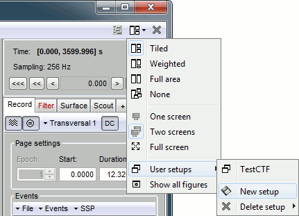
This preparation of the reviewing environment requires a large number of operations, and would become quickly annoying if you have to repeat it every time you open a file. This is a good time to use the menu "User setups" to save this window configuration, so that you can reload it in one click later. In the menu "Window layout", at the top-right of the Brainstorm window, select User setup > New setup. Enter a name of your choice for this particular window arrangement.
This operation will also disable the automatic window arrangement (Window layout > None). To reload it later, open one figure on the dataset you want to review and then select your new entry in the User setup menu.
Multiple montages
It may be interesting for some cases to display different groups of sensors in multiple windows (eg. with an MEG system with 300 sensors), or some complicated epilepsy cases where you would like to review at the same time multiple montages (eg. longitudinal and transversal bipolar montages). Brainstorm offers a flexible way of doing this.
Open your full reviewing environment as described before, where the EEG signals are displayed with the "Average reference" montage.
Open another view on the same data with the "Longitudinal 3" montage ("double-banana" LB-18.3)
Right-click on the "Link to raw file" again > EEG > Display time series
Alternatively, you can right-click on the existing figure > Figure > Clone figure.
- Then set the montage for this new figure to "Longitudinal 3"
- Redimension all the figures to make room for the new window
- Save this as a new "User setup"
- If you don't see the "Longitudinal 3" menu, it is probably because you have using Brainstorm before these predefined montages were made available in the software distribution. To add them manually:
- In the Record tab, select "Edit montages" in the drop-down menu
- Click on the "Load montage" button
- Go to the folder "brainstorm3/toolbox/sensors/private/", and select the first file
- Note that a new entry (probably "Longitudinal 1") is added to the list of available montages
- Repeat the operation with all the files in the folder "brainstorm3/toolbox/sensors/private/"
- Click on "Save" to close the montage editor and now select "Longitudinal 3"
Mark spikes
In this dataset, some single spikes have already been identified by experts at the University Hospital of Freiburg. You can see that 58 SPIKE events are available in the Record tab. Click on a few of them and try to identify the shape of the spike.
The procedure if you are marking the events by yourself is the following:
- Close all the current figures ("Close all" button at the top-right corner of the Brainstorm window)
- Double-click on the "Link to raw file" to open a continuous file viewer, and load your reviewing environment (menu User setups)
Start by creating a group of events (Events > Add group), and select it in the list of events.
Make sure that the time and amplitude resolutions are what you are used to
(right-click on the figure > Figure > Set axes resolution)Scroll through the recordings using the [<<<] and [>>>] buttons or shortcuts such as F3 or F4 (complete list and descriptions available when you leave your mouse over these buttons).
You can adjust the gain of the electrodes to observe better an event with the buttons [^] and [v], with the keyboard (+/-) or the mouse ([Shift+mouse wheel] or [Right-click+move up/down]).
- When you identify a spike, click in a white area of the figure in order to place the time cursor at the peak of the spike. If you click on the signal itself, it selects the corresponding channel, but you can use the shortcut Shift+Click to prevent this behavior and force the time cursor to be moved instead.
- Press Ctrl+E to add a marker where the time cursor is.
If you are marking multiple types of events, it is convenient to set up some additional keyboard shortcuts. Using the menu Events > Edit keyboard shortcuts, you can associate custom events to the key 1 to 9 of the keyboard. Define the name of the event type to create for each key, and then simply press the corresponding key to add/delete a marker at the current time position.
- To jump to the next/previous event in the current category: use the keyboard shortcuts [Shift+arrow right] and [Shift+arrow left]
More information on the data viewer, see tutorial: Review continuous recordings.
Pre-process recordings
Average reference
Evaluation
Two of the typical pre-processing steps consist in getting rid of the contamination due to the power lines (50 Hz or 60Hz) and of the frequencies we are not interested in (a low-pass filter to remove the high-frequencies and a high-pass filter to remove the very slow components of the signals). Let's start with the spectral evaluation of this file.
Drag the "Link to raw file" to the Process1 box and run the process "Frequency > Power spectrum density (Welch)". Configure it as illustrated in the following figure (window length=10s, overlap=50%).
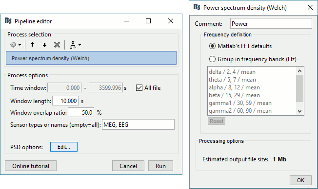
Double-click on the new PSD file to display it.
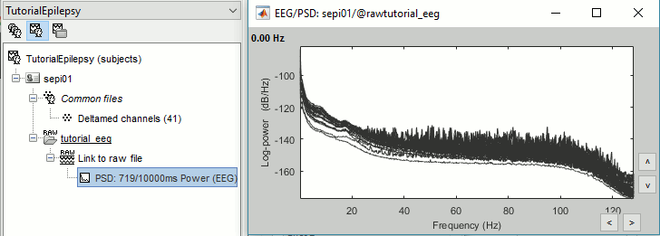
This frequency spectrum does not show any particular peak at 50/60Hz, there is no notch filter to apply on these recordings. If we had to, we would run the process "Pre-processing > Notch filter" as explained in the tutorial Detect and remove artifacts.
Band-pass filter
We would like to apply a band-pass filter to keep only the frequencies between 0.5Hz an 80Hz. The high-pass filter at 0.5Hz will rid of the slow amplitude fluctuations (longer than 2s).
- Leave the "Link to raw file" selected in the Process1 list.
Run the process "Pre-process > Band-pass filter", with the options:
Lower cutoff frequency: 0.5 Hz (high-pass filter)
Upper cutoff frequency: 80 Hz (low-pass filter)
Mirror signal before filtering: On
Sensor types: EMPTY (to process all the signals)
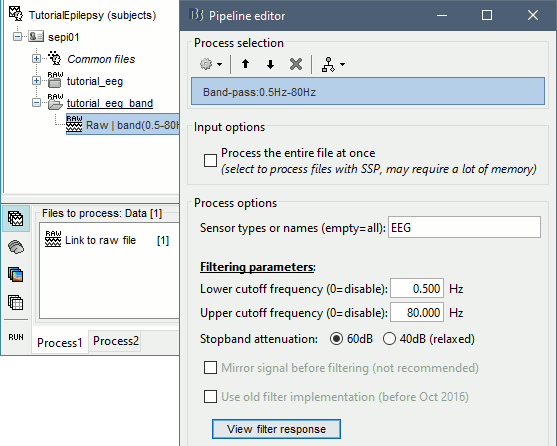
- Note that this new continuous files is saved in your Brainstorm database, while your original file is saved in a separate folder (sample_epilepsy). If you delete the link to the original file with the database explorer, it would not delete the actual file. If you delete the link to the filtered file, it would delete the file itself.
- Drag this new file "Raw | band(0.5-80Hz)" to the Process1 list.
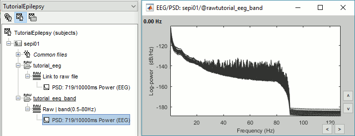
Run again the process "Frequency > Power spectrum density (Welch)", with same options as before.
Double-click on the new PSD file to display the spectrum of the filtered file.
Epoching and averaging
Import recordings
- Now we want to extract all the spikes as 400ms windows from this filtered file.
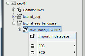
Right-click on the imported and filtered file "Raw (0s,3600s) | high(0.5Hz)" > Import in database
Select the option "Use events" and select the category SPIKE, with 58 events.
Epoch time: [-100, +300]ms around the spike events
Uncheck "Remove DC offset": the DC offset has already been removed with the high-pass filter
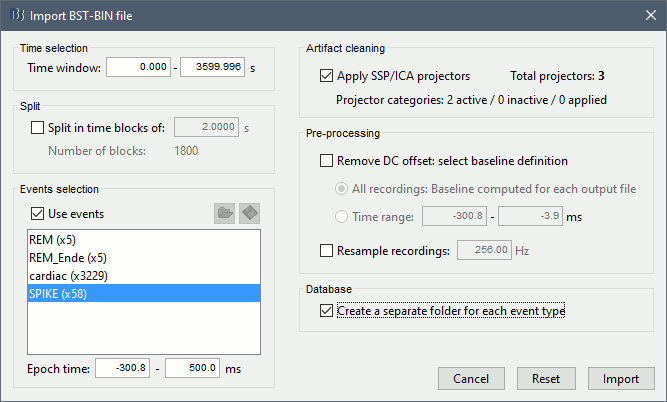
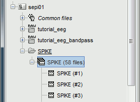
You should see a new folder "SPIKE" containing 58 epochs in your database.
Average spikes
- Drag and drop all the SPIKE files or the SPIKE folder into the Process1 tab
Run the process "Average > Average files", with the following options:
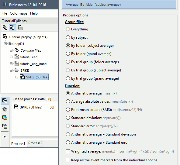
- Double click on the new file "Avg: SPIKE" to review it, and set the "Average reference" montage.
Go to the Filter tab to disable all the visualization filters: these filters are not working well on short signals, the high-pass filter at 0.5Hz can introduce errors in the display of the average.
Open a "2D sensor cap" view on the same file, or simply press [Ctrl+T] from the time series figure.

- To have all the figures automatically re-arrange themselves again, select "Weighted" or "Tiled" in the "Window layout" menu (top-right corner).
- Explore this average in time with the left and right keyboard arrow.
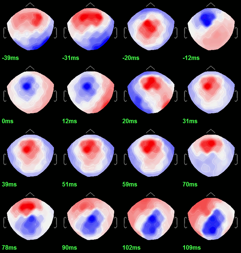
Typically, the analysis could be limited to the ascending part of the peak (from -11ms to 0ms), as it gives a rather clear information on the primary epilepsy focus. For the rest of the tutorial, we will use a larger time window (-40ms to 100ms) in order to illustrate the visualization tools. Just keep in mind that it can be hazardous to interpret waves that are far in time or in space from the primary focus.
- To get a synthetic view at the sensor level of the evolution of the 2D map in time:
Rright-click on the figure > Snapshot > "Time contact sheet: Figure"
Set the time window [-40ms, 110ms], with 16 images
Source analysis: Cortically constrained
Head model
We are going to use a realistic head model, this requires to calculate some additional surfaces for the subject, to represent the inner skull and outer skull surface. Go to the "Anatomy" view, right-click on the subject > Generate BEM surfaces.
Use 1922 vertices for each layer (default). Three new surface files are created at the end:
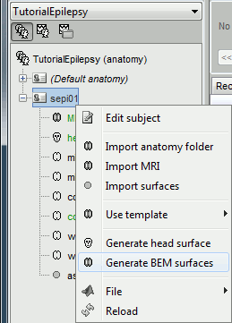
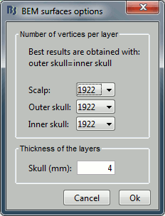
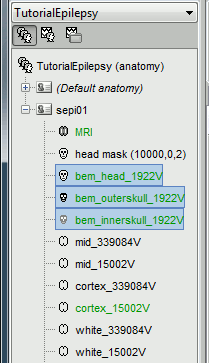
Go back to the "Functional data" view, right-click on the channel file (or any folder containing the channel file) > Compute head model
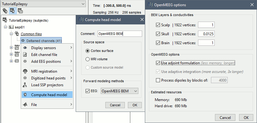
Select the "cortex surface option" and the "OpenMEEG BEM" forward model. Leave all the OpenMEEG options to their defaults except for one: select the option "Use adjoint formulation".
![[ATTACH] [ATTACH]](/moin_static1911/brainstorm1/img/attach.png)
![[ATTACH] [ATTACH]](/moin_static1911/brainstorm1/img/attach.png)
- If the automatic download doesn't work, download and install OpenMEEG manually (menu Help)
If the OpenMEEG calculation crashes, please refer to the OpenMEEG tutorial.
- If you can compute the model but then later the source maps you get don't make any sense, it is probably because the BEM surfaces were poorly defined. When some cortex vertices are too close to the inner skull surface, the model can be unstable and after the source estimation you would typically see source maps containing zeros everywhere except for a few vertices. If this happens, delete the existing BEM surfaces and try computing new ones with a higher number of vertices for the inner and outer skull BEM surfaces.
If you cannot get OpenMEEG to work, or if the results definitely do not make sense, try using a different forward model: "3-shell sphere". It's a spherical model, so it would perform better in the regions of the head that are close to the sphere. See the Head model tutorial.
Noise covariance matrix
For minimum norm inverse models, we need to estimate first the level of noise at the level of the sensors. Defining what can be considered as "noise" in the middle of continuous brain recordings is a difficult question, discussed in the Noise covariance tutorial.
- Here we chose what is described as option 1b in the section "Noise and epilepsy" in that tutorial: we are going to calculate the noise covariance matrix using 10 seconds from the continuous file that are very "quiet", ie. that contain no apparent epileptic activity, no REM and no other special artifacts. We can use for this purpose the 10s segment between 120s and 130s.
- The file you use for the calculation of the noise covariance matrix must be pre-processed in the same way as the files for which you want to estimate the sources (the SPIKE epochs), so we need to use the imported+filtered continuous file.
Right-click on the "Raw (0s,3600s) | high(0.5Hz)" > Noise covariance > Compute from recordings
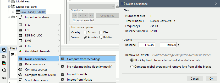
Select the time window [120s - 130s] and leave the other options to the default values
![[ATTACH] [ATTACH]](/moin_static1911/brainstorm1/img/attach.png)
Inverse model
Right-click on the head model > Compute sources.
Leave all the default options to calculate a wMNE solution with constrained dipole orientation
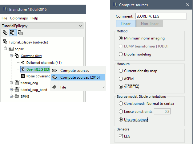
This operation creates a shared inversion kernel in the folder (Common files) and one source link for each block of recordings in subject sepi01. If you are not familiar with these concepts, please refer to the Source estimation tutorial.

Double-click on the sources file for the average to open it. Configure its display: surface smoothing, amplitude threshold, colormap. For a reminder on how to manipulate the colormaps, see the tutorial Colormaps.
- Make sure that all the visualization filters are turned OFF.
Double-click on the recordings as well to get a visual reference of the time. In the Record tab, you can click on the "Display mode" button in the toolbar to switch back to the "butterfly" view.
![[ATTACH] [ATTACH]](/moin_static1911/brainstorm1/img/attach.png)
To display the same information re-interpolated in the volume, right-click on the source file > Cortical activation > Display on MRI
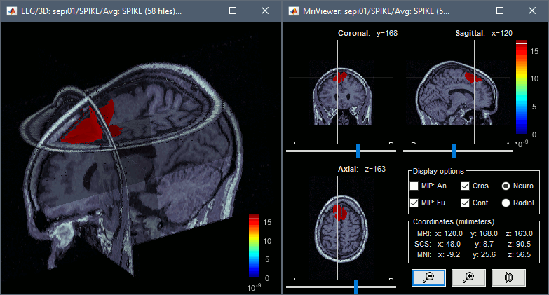
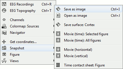
You can save movies or contact sheets of the source maps with the Snapshot popup menu
Example: Video made with three figures: Download
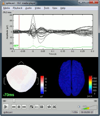
- The inverse solutions that you calculated are all shared for all the recordings in this subject, so you can go back to your individual epochs, or even the continuous file, and look at the source maps for these files.
Regions of interest
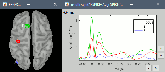
- The scouts are a very interesting feature for studying the spike spatial propagation. From the displays we generated previously, there is no clear propagation of the spike. Let's try to explore this in more details, at least to illustrate the method.
- Start by placing a small scout at the focus (~7 vertices)
- Place a few other scouts of a similar size at other places around the spike location, in places at which you could suspect a possible propagation.
- Plot the overlayed time series for these scouts. Try with the scout functions MEAN and MAX.
- There is no delay in the peaks for the different regions at -20ms, 0ms and 35ms This temporal exploration seems to confirm that there is no clear spatial propagation of the spike.
If you need a reminder on how to manipulate scouts: see the Scouts tutorial
Z-score normalization
A good way to reveal better the source activity at the cortex level is to calculate a Z-score of the source maps with respect with a quiet baseline. We can use the same baseline as for the calculation of the noise covariance matrix.
Import the block a recordings to use as the baseline. Right-click on the imported and processed file "Raw (0s,3600s) | high(0.5Hz)" > Import in database. Uncheck all the options and select the time window: [120, 130] secondes.
![[ATTACH] [ATTACH]](/moin_static1911/brainstorm1/img/attach.png)
- Click on the Process2 tab
- In Files A: Drag the sources for the segment you just imported "Raw (120.00s,130.00s)"
- In Files B: Drag the sources for the averaged spike
Alternatively, select the recordings and manually select the "Process sources" button on both sides
![[ATTACH] [ATTACH]](/moin_static1911/brainstorm1/img/attach.png)
Run the process: Standardize > Z-score (static). Double-click on the new file to display it
![[ATTACH] [ATTACH]](/moin_static1911/brainstorm1/img/attach.png)
![[ATTACH] [ATTACH]](/moin_static1911/brainstorm1/img/attach.png)
- The amplitude in the figure is now displayed without units, it represents a multiple of the standard deviation over the baseline. The interpretation of this new figure is not very different from the previous one, but it helps observing the things with a different angle. This process usually provides smoother maps, with less bias due to the depth of the sources. On the non-standardized minimum norm maps, the values of the deeper sources are usually lower than the ones at the surface. The Z-score helps showing deeper sources that have minimum norm values that are low, but higher than during the baseline.
Source analysis: Full head volume
If the results you obtain are not satisfying with the surface-based source estimation, you can run again the same analysis with a different source space, sampling the entire head volume instead of being constrained to the surface. More information about this method in the Volume source estimation tutorial.
Head model
Right-click on the channel file > Compute head model, select "MRI volume" instead of "Cortex surface". This feature is now stable, but still tagged as experimental because not all the Brainstorm features are available for volume-based source models (eg. no regions of interest, no group analysis, etc). Use the same options as before for OpenMEEG.
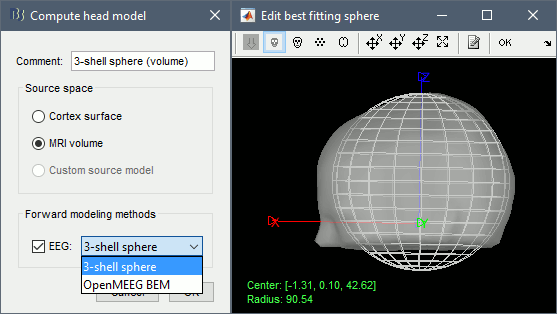
![[ATTACH] [ATTACH]](/moin_static1911/brainstorm1/img/attach.png)
Inverse model
Right-click on the head model > Compute sources. Use all the default options.
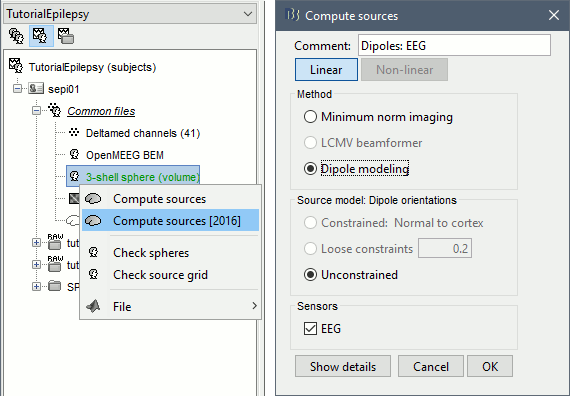
Right-click on the unconstrained sources > Cortical activation > Display on MRI (3D).
Right-click on the same file > Cortical activation > Display on MRI (MRI Viewer)
Moving dipoles
See tutorial: Computing and displaying dipoles
Note: you can also load dipoles calculated with other programs.
MEM inverse solution
This section is on a different page: ?Link
Discussion
Distributed source models vs. ECD (equivalent current dipole)
Kobayashi K, Yoshinaga H, Ohtsuka Y, Gotman J (2005)
Dipole modeling of epileptic spikes can be accurate or misleading
Epilepsia, 2005 Mar;46(3):397-408.
Distributed source models vs. BOLD
Heers M, Hedrich T, An D, Dubeau F, Gotman J, Grova C, Kobayashi E (2014)
Spatial correlation of hemodynamic changes related to interictal epileptic discharges with electric and magnetic source imaging. Human Brain Mapping, published online 24 Feb 2014.
ECD vs. BOLD
Benar CG, Grova C, Kobayashi E, Bagshaw AP, Aghakhani Y, Dubeau F, Gotman J (2006)
EEG–fMRI of epileptic spikes: Concordance with EEG source localization and intracranial EEG
NeuroImage, 30:1161-1170.
Forum posts
Scripting
To reproduce this entire analysis with a script, use the following processes:
Import recordings > Import anatomy folder
Subject name: sepi01
Folder to import: sample_epilepsy/anatomy (format = FreeSurfer)
- Enter the fiducials positions indicated at the beginning of the tutorial
- Because of the selection of these points, it is usally better to run this first step in interactive mode.
Import anatomy > Generate BEM surfaces
- Set all the values to 1922 and the skull thickness to 4mm
Import recordings > Create link to raw file
File to import: sample_epilepsy/data/tutorial_eeg.bin (format = Deltamed Coherence-Neurofile)
- Uncheck the option "Align sensors using headpoints"
Import recordings > Set channel file
File to import: sample_epilepsy/data/tutorial_electrodes.elc (format = EEG:ANT Xensor)
- Check the option "Align sensors using headpoints"
Import recordings > Project electrodes on scalp
Import recordings > Set channels type
Channel types or names: SP1, SP2, RS, PHO, DELR, DELL, QR, QL
Events > Import from file
Event file: sample_epilepsy/data/tutorial_spikes.txt: (format = Array of times)
Event name: SPIKE
Import recordings > Import MEG/EEG: Time
- Condition name: Empty
- Time window: default (entire file)
- Split recordings in time blocks: 0s
Pre-process > Band-pass filter:
Lower cutoff frequency: 0.5 Hz
- Upper cutoff frequency: 0
- Sensor types: Empty
Check: Overwrite input file
Sources > Compute noise covariance
Baseline: [120s - 130s]
- Remove DC offset: Block by block
- Ouptut: Full noise covariance matrix
Import recordings > Import MEG/EEG: Events
- Condition name: Empty
Event names: SPIKE
- Time window: default (entire file)
Epoch time: [-101.6s, 300.8s]
- Check all the additional options
Average > Average files
- By condition (subject average)
- Arithmetic average
- Uncheck: Keep all the events
File > Save snapshot
- Snapshot: Sensors/MRI registration
- Sensor type: EEG
- Orientation: Left
- Comment: "Average spike"
File > Save snapshot
- Snapshot: Recordings time series
- Sensor type: EEG
File > Save snapshot
- Snapshot: Recordings topography (contact sheet)
- Sensor type: EEG
- Contact sheet (start time, stop time): "-40 110"
- Contact sheet (number of images): 16
Sources > Compute head model
- EEG Method: OpenMEEG BEM
- Edit OpenMEEG options
- BEM Layers: Select all (scalp, skull, brain)
- Check: Use adjoint formulation
- Check: Use adaptive integration
Sources > Compute sources
- wMNE
- Sensor types: EEG
- Kernel onle: Shared
File > Save snapshot
- Snapshot: Sources (one time)
- Orientation: top
- Time: 0s
The following script from the Brainstorm distribution reproduces the analysis presented in this tutorial page: brainstorm3/toolbox/script/tutorial_epilepsy.m

