Specparam/Fitting Oscillations and One-Over-F (FOOOF)

Authors: Luc Wilson, Jason da Silva castanheira, Raymundo Cassani

This tutorial introduces the features developed in Brainstorm to compute and view FOOOF models from a Welch’s Power Spectral Density (PSD) file.

Note: The FOOOF algorithm has recently been renamed by its authors to specparam.

Introduction

The Fitting Oscillations and One-Over-F (FOOOF/specparam) algorithm is designed to identify and model features of the neural power spectrum. It performs a sequential decomposition of the power spectrum into aperiodic and periodic components, optimizing the modelled spectrum using a least-squared-error approach. The present tutorial will demonstrate the algorithm’s functionality within the Brainstorm interface; for a detailed breakdown of the algorithm, please refer to the FOOOF GitHub.

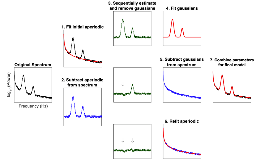
This demonstration uses sample data from the introduction dataset, and can be followed by completing all steps of the Brainstorm tutorial up to and including tutorial 10.

Initializing and running FOOOF

FOOOF is principally performed on Welch’s PSD files. Analysis of Fourier transforms are also possible, but not recommended. We will run FOOOF over the PSD files we previously produced.

• Clear the list of files in the Process1 tab.
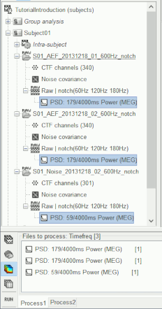
• Select the PSDs from the three datasets we have linked to our protocol and load them into Process1.

  You can select the two "PSD: 179/4000ms Power (MEG)" files and the single "PSD: 59/4000ms Power (MEG)". If you do not have these PSDs, refer to tutorial 10.

• Click on [Run] to open the pipeline editor window.

• Select the process "Frequency > FOOOF: Fitting oscillations and 1/f".
  
  

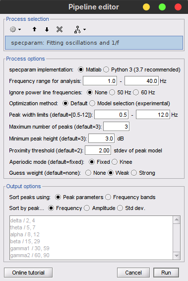
Select the following process options:

• FOOOF version: Matlab
  This option allows you to choose which version of FOOOF you would like to run; either the MATLAB standalone version, or the original Python version. Results and computation times may vary slightly between versions but are roughly the same.

• Frequency range for analysis: 1.0 - 40.0 Hz [default: 1.0 - 40.0 Hz].
  FOOOF is best performed on a subset of the frequencies from the original PSD. In this range, it is important to avoid frequencies which have previously been filtered, as their adjusted powers can alter model results adversely.

• Ignore power line frequencies: None [default: 60 Hz].
  Depending on whether a notch filter was previously used for one's regional power line frequency (and harmonics), FOOOF may either be attempting to fit increases in power attributable to power lines as peaks, or the aperiodic fit may be disrupted by 'negative peaks' of power. To avoid both of these pitfalls, users can choose to ignore frequencies whose power measures have been disrupted by power lines or their filtering (for instance, 60±2Hz, 120±2Hz, 180±2Hz) in the modelling process. This option becomes important when fitting a broader range of frequencies (>40Hz) and should be set in accordance with one's region.

• Peak model: Gaussian [default: Gaussian].
  The original FOOOF algorithm fits spectral peaks using a gaussian distribution; the MATLAB version also allows the algorithm to fit peaks using a Cauchy distribution instead. The final option ("Best of Both") allows for individual channels to be fit using the distribution which minimizes model mean squared error (MSE).

• Peak width limits: 1.5 - 12.0 Hz [default: 0.5 - 12.0 Hz].
  The bounds for a putative peak to be included in the final FOOOF model. Putative peaks outside these bounds are discarded.

• Maximum number of peaks: 3 [default: 3].
  The maximum number of attempts the model will make to identify peaks; it is best to allow for at least the number of observable peaks in the PSD plus one, in the event that the model does not remove a larger peak entirely in the peak-identification process.

• Minimum peak height : 3.0 dB [default: 3 dB].
  The minimum peak height (in log[Power]) necessary for a putative peak to be included in the final FOOOF model. Putative peaks smaller than this threshold will be discarded.

• Proximity threshold: 2 standard deviations of the (comparatively) largest peak [default: 2].
  Occasionally, the algorithm can mistake components of a single peak as two smaller peaks. This option forces the smaller of two peaks which are too close to one-another (i.e. If the center frequency of the smaller peak is within this value of standard deviations of the larger peak’s center frequency), the smaller of the two peaks is discarded. This option also removes peaks within this value of their standard deviation from the edge of the frequency window.

• Aperiodic mode: Fixed [default: Fixed].
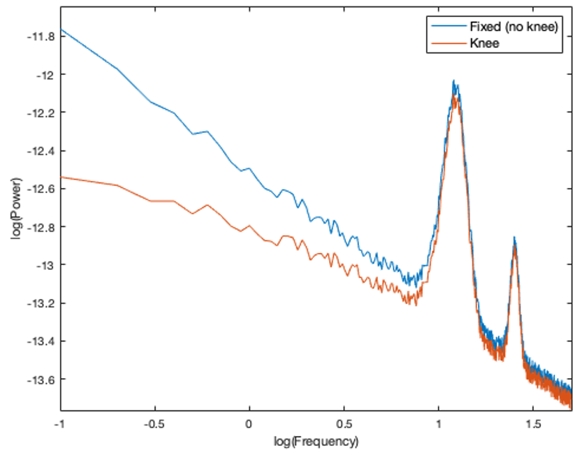
  The aperiodic component of the neural power spectrum occasionally presents with a knee, as seen below in log-log space. When selecting this option, you should first consult your data to determine whether it has a knee or not (Note: a knee component is present when the aperiodic features of the spectrum plotted in log-log space are not linear).
  
  

• Guess weight: Weak [default: None].
  By design, peak parameter estimates are close to the actual fit. However, fitting a distribution that does not match the spectrum precisely (i.e. fitting a gaussian distribution to an imperfect gaussian-shaped peak) can occasionally lead to semantically worse-fit models; square error is reduced, but the model does not look as much like the data. Selecting this option allows for additional model error to be placed on parameter values which lie further from initial estimates. “Weak” represents a small penalty, while “Strong” represents a larger penalty (essentially keeping the pre-optimization estimates). When this option is set to “None”, the algorithm reduces square error most similarly to the Python version.

  • Note: Guess weight selections are ignored when Brainstorm detects that the user has the optimization toolbox, as it will use constrained optimization to best-match the Python version. It is recommended that users have the optimization toolbox.

Select the following output options:

• Sort peaks using: Peak parameters

  • This sorts peaks according to a particular property of the peaks, defined below.

• Sort by peak: Frequency.

  • This sorts peaks by center frequency, in ascending order. (If you would not like to rearrange peaks, sort peaks using frequency bands).

Viewing FOOOF models

Three new files should now be visible, with one below each PSD we just processed.

• Double-click on the first new file to open the spectrum figure.

• When viewing the options in “Display”, you should see a new set of options specific to FOOOF, including Spectrum (the original PSD), FOOOF Model (the new FOOOF model), Aperiodic only (which plots only the model’s aperiodic component), and Peaks only (which plots only the model’s peak components).
  
  

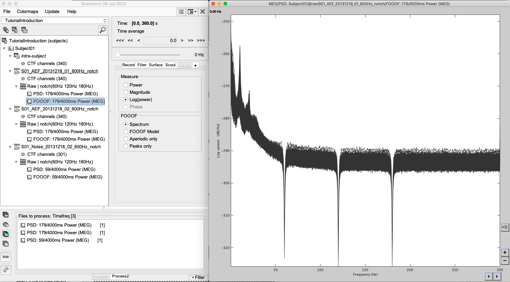
• Try all the display options:
  
  

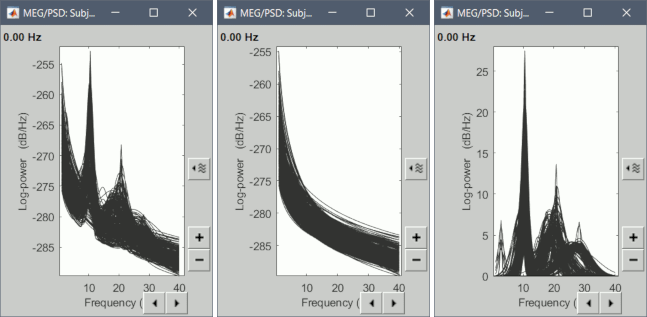
This is an ideal environment to view FOOOF models to ensure that they are fitting the spectrum correctly. Here, you can also double-click and view the original PSD file at the same time, selecting individual channels to determine goodness-of-fit qualitatively.

Accessing FOOOF model parameters

While viewing the FOOOF models within Brainstorm is helpful for qualitative interpretations, some may wish to extract the parameter values directly from the model for statistical tests.

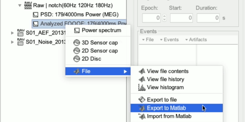
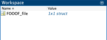
• Right-click on the first FOOOF file and select "File > Export to Matlab". Name the variable anything you would like (eg. "FOOOF_file").
  
  

• In MATLAB, you can explore the contents of the file using the tab "Workspace" (navigate to "FOOOF_file > Options > FOOOF") or the command line (FOOOF_file.Options.FOOOF).
  

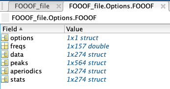
• The FOOOF structure contains six additional elements:

  • options: all of the settings for the algorithm.

  • freqs: all of the specific frequencies used in the model.

  • data: channel-specific FOOOF models, in the same order as present in Brainstorm.

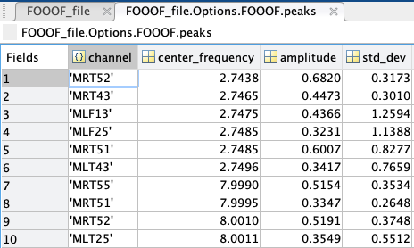
  • peaks: a struct containing every peak’s channel of origin, center frequency (in Hz), amplitude (in B, Bells, or log[Power]), and standard deviation/gamma (in Hz); if peaks were sorted by frequency band, another column would show the name of the frequency band the peak is located in.
    
    

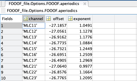
  • aperiodics: a struct containing every channel’s aperiodic slope (exponent) and broadband offset (in B, Bells, or log[Power]); if aperiodic mode was set as “Knee”, another column would show the knee frequency of the aperiodic.
    
    

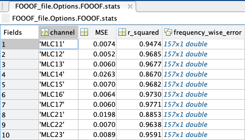
  • stats: a struct containing every model’s channel of origin, MSE, R-squared, and absolute frequency-wise error.
    
    

Convert FOOOF model parameters to regular PSD files

You can convert parameters of a FOOOF model to regular PSD files. This can be useful, as it allows using all the processes for PSD on FOOOF model parameters. For example, to export FOOOF model parameters as SPM surfaces,SPM volumes, group in frequency bands, etc.

• In Process1: Select the FOOOF model file.

• Run process: "Frequency > specparam: Extract measure":

  • specparam meaure: Peaks only

• 

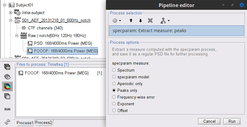
• A new file with the same name but without the "| peaks" tag is created. This file is a regular PSD file that you can use with any process. When you open it, the FOOOF options do not show up.

Python implementation

Some process options are only available in the MATLAB version. They have been added to allow for greater flexibility in the algorithm’s settings; a few are actually within the Python version, but are inaccessible via MATLAB.

If you would prefer to use the algorithm in its original state, you can instead select FOOOF version: Python. To use the Python version, some configuration of your system is required.

• To direct MATLAB to the correct Python executable, use the function pyenv (>= 2019b) or pyversion (=< 2019a) after starting up MATLAB. Read this blog post for more information.

• You must have also downloaded and installed SciPy, NumPy, and FOOOF Python libraries on your computer (installation instructions).

• Your Python environment must be available in your system path. It should always be the case by default on Linux and MacOS, but not necesarily on Windows. You might have to add some folders to your system path (instructions). The folders to add depend on your Python distribution, but could be something like:

• C:\Users\username\Anaconda3\envs\mne;C:\Users\username\Anaconda3\envs\mne\Library\mingw-w64\bin;C:\Users\username\Anaconda3\envs\mne\Library\bin;C:\Users\usernamec\Anaconda3\condabin;C:\Users\username\Anaconda3\Scripts

Model-selection (ms-specparam)

The current available tools to neuroscientists for parametrizing brain activity, rely on user expertise. Users are required to tune the hyperparameters of specparam/FOOOF model in order to achieve an optimal fit. In the following section, we introduce model-selection spectral parametrization (ms-specparam) algorithm which adjusts progressively more complex models to the spectrum to achieve the most parsimonious fit. This novel implementation of specparam/FOOOF uses data-driven model selection to minimize the reliance on user expertise and subjective choices, enabling more robust, reproducible, and interpretable research findings.

The hyperparameters of specparam/FOOOF are method parameters that help the algorithm fit the neural power spectrum to the data. An example of such a hyperparameter is the maximum number of Gaussian peaks to fit (see Initializing and running FOOOF).

The choice of hyperparameter can significantly modify the resulting spectral model and its interpretation. Take for example the spectrum presented in the Figure below. The user-dependent choice in the maximum number of number of peaks expected from spectral parameterization was set manually to a value of 6. Under high signal-to-noise conditions (presented on the left), spectral parameterization may yield only two peaks as expected. In noise conditions more closely aligned with real data, however, the spectral parameterization algorithm may overestimate the number of peaks in the spectrum to account for noise-related fluctuations (example on the right). This difference in the number of estimated peaks alters the interpretation of the resulting spectral model.

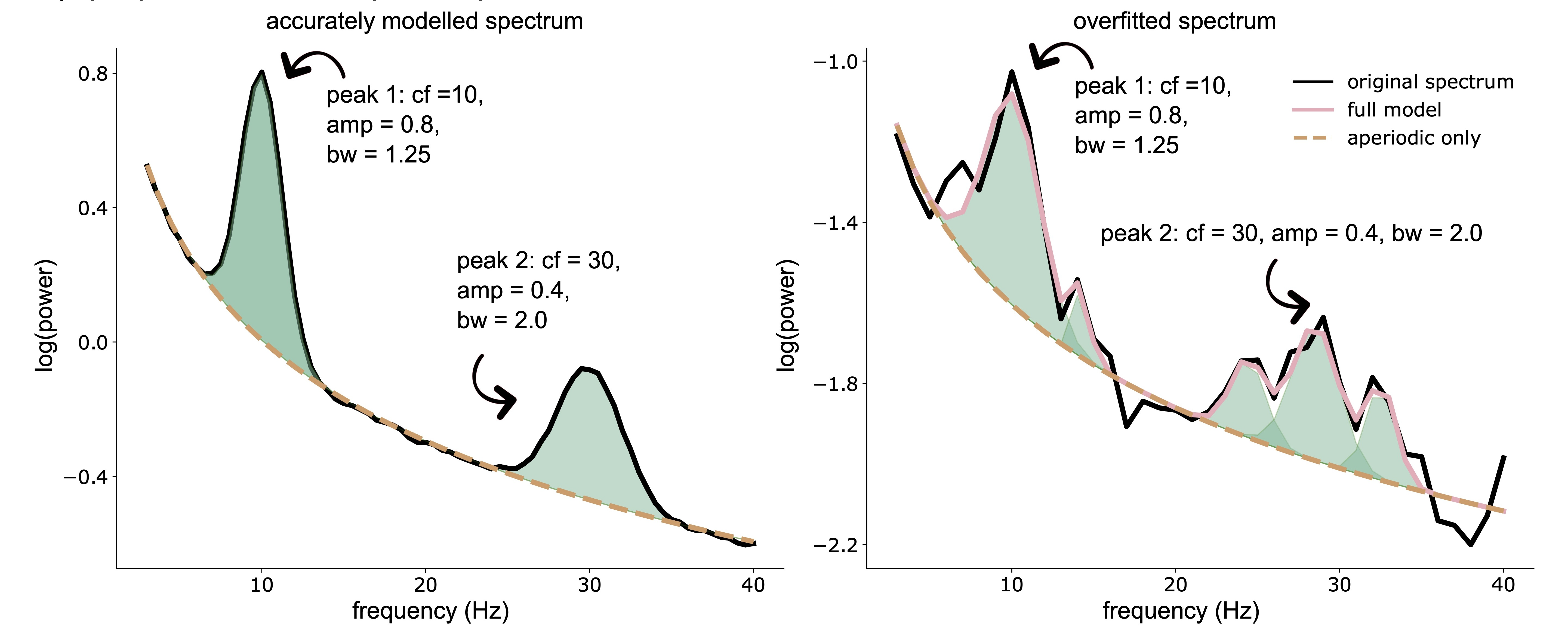
• The illustration above depicts an example spectral parameterization of a simulated power spectral density estimate (black line) obtained with specparam in the context of lower (left panel) and higher (right panel) noise levels. Both spectra are generated using the same spectral parameters (i.e., two spectral peaks). In more noisy conditions, specparam (pink line) fits a greater number of spectral peaks (green shaded areas) than what is present (simulated) in the data, resulting in overfitting (right panel). Key: ‘cf’ refers to a peak’s center frequency, ‘amp’ refers to a peak’s amplitude, and ‘bw’ refers to a peak’s bandwidth.

To automatically and adaptively adjust model hyperparameters to account for the noise level in the data, we introduce the model-selection strategy. The ms-specparam method proceeds with adjusting progressively more complex models to the empirical data spectrum or spectrogram, and determines the parameters of the simplest model that adequately accounts for the data. Ms-specparam selects the best model by accounting for both the best fitting model, while also picking the most parsimonious model (i.e., fewest spectral peaks) using the Bayesian information criterion (BIC). See Figure below for algorithm's pipeline.

In Wilson and colleagues (2024), we present extensive tests of the approach with ground-truth and empirical magnetoencephalography recordings and demonstrate that ms-specparam shows enhanced specificity and sensitivity of spectral and spectrogram decompositions, even when used as part of Spectral Parameterization Resolved in Times (SPRiNT).

Ms-specparam, like FOOOF, is principally performed on Welch’s PSD files. Analysis of Fourier transforms are also possible, but not recommended. Below we will run ms-specparam over the PSD files we previously produced.

• Clear the list of files in the Process1 tab.
• Select the PSDs from the three datasets we have linked to our protocol and load them into Process1.

  You can select the two "PSD: 179/4000ms Power (MEG)" files and the single "PSD: 59/4000ms Power (MEG)". If you do not have these PSDs, refer to tutorial 10.

• Click on [Run] to open the pipeline editor window.

• Select the process "Frequency > BIC-FOOOF".
  
  

Note that ms-specparam has similar process options and FOOOF structure as described above.

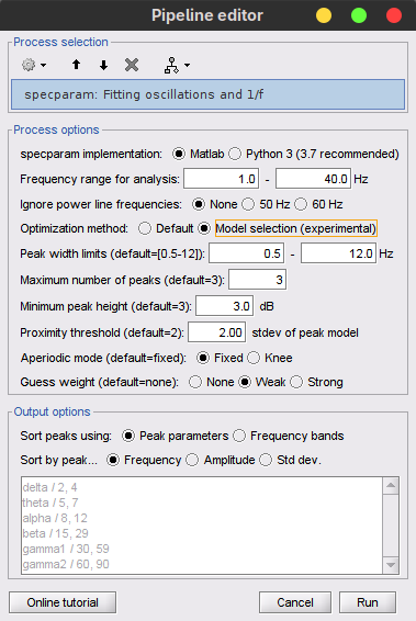
As ms-specparam relied on the Bayesian information criterion (BIC), this also enables the quantification of evidence for periodic activity in spectral data via Bayes factor analysis. The best fitting model as determined by BIC is utilized in a Bayes factor inference against the aperiodic only spectral model (panel i of figure below). This analysis helps users adjudicate whether spectral peaks are likely to be present in the data power spectrum. A Bayes factor less than 1 is evidence in favour of periodic brain activity over the null hypothesis of no periodic brain activty (panel iv). In contrast, a Bayes factor greater than 1, is evidence in favour of no periodic activity (i.e., the null hypothesis).

Summary

FOOOF is an algorithm designed to complement many analytical techniques already in use today. Its purpose is to help researchers characterize the neural power spectrum more quantitatively; it is not necessarily meant to be used for exploratory means. The algorithm can return noticeably different models depending on whether the settings provided are suitable for the spectra being parametrized. Understanding the characteristics of a particular power spectrum is crucial to modelling them appropriately. The best way to determine whether a model is appropriate for a given spectrum is to compare the original and modelled spectra side-by-side.

Acknowledgements

All credit for the conception of the original FOOOF algorithm is due to Thomas Donoghue, Matar Haller, Erik Peterson, Paroma Varma, Priyadarshini Sebastian, Richard Gao, Torben Noto, Antonio H. Lara, Joni D. Wallis, Robert T. Knight, Avgusta Shestyuk, and Bradley Voytek. The appropriate citation for FOOOF is as follows:

Donoghue, T., Haller, M., Peterson, E.J. et al. Parameterizing neural power spectra into periodic and aperiodic components. Nat Neurosci 23, 1655–1665 (2020). https://doi.org/10.1038/s41593-020-00744-x

Luc E. Wilson, Jason da Silva Castanheira, Benjamin Lévesque Kinder, Sylvain Model selection for spectral parameterization. BioRxiv (2024). https://www.biorxiv.org/content/10.1101/2024.08.01.606216v1