|
Size: 356
Comment:
|
Size: 10012
Comment:
|
| Deletions are marked like this. | Additions are marked like this. |
| Line 2: | Line 2: |
| ''Authors: Francois Tadel, Elizabeth Bock, John C Mosher, Sylvain Baillet'' | ''Authors: Francois Tadel, John C Mosher, Richard Leahy, Sylvain Baillet'' This tutorial is still based on Sabine Meunier's somatotopy experiment, called ''TutorialCTF ''in your Brainstorm database. The recordings have already been imported and analyzed at the sensors level, they are ready for source estimation. |
| Line 6: | Line 8: |
| == Forward problem == The first step consists in computing a model that explains how an electric current flowing in the brain can influence what is recorded out of the head, by the EEG or MEG sensors. * This problem is called forward problem. * Its result is called ''head model ''in Brainstorm interface, but can also be referred as ''forward model'' or ''leadfield matrix''. * In the Brainstorm software, we consider by default that the electric or magnetic activity which is recorded by the sensors is produced mainly by a set of electric dipoles located at the surface of the cortex.<<BR>> * The grid of sources (dipoles) that is used is defined by the cortex surface we have imported in one of the previous tutorials; each vertex of this surface is considered as a dipole. * The default surface distributed with Brainstorm have around 15,000 vertices. So we will have 15,000 dipole amplitudes to estimate. Using less vertices would just lower the resolution of the results; using more produces too much data and might lead to memory issues. * What we expect to get at the end of this process is a matrix whose size is [Number of sensors x Number of sources] * For computing this matrix, three methods are available for MEG recordings in Brainstorm: * '''Single sphere''': the head is considered a homogeneous sphere * '''Overlapping spheres''': Refining the previous model by fitting one local sphere for each sensor * '''OpenMEEG BEM''': Symmetric Boundary Element Method from the open-source software OpenMEEG. Described in an advanced tutorial: [[Tutorials/TutBem|BEM head model]]. {{attachment:forwardInverse.gif}} == Single sphere model == Select the ''TutorialCTF ''protocol, close all the figures, and follow these steps: 1. Right-click on the ''Right'' condition and select ''Compute head model''. The ''Head modeler'' window will appear.<<BR>><<BR>> {{attachment:popupHeadModel.gif}} --- {{attachment:headModeler.gif}} 1. Set the options for your head model: * Source space: '''Cortex surface'''. <<BR>>The MRI volume option will be introduced in an advanced tutorial: [[Tutorials/TutVolSource|Volume source estimation]]. * Forward modeling method: '''Single sphere'''. * You can also edit the '''Comment '''field of the file that will be created (the string that will be representing the head model in the database explorer). * Click on ''Run''. 1. Two other windows appear, to help you define the sphere. Estimating the best fitting sphere for a head is not always as easy as it looks like, because a human head is usually not spherical. <<BR>><<BR>> {{attachment:helpBfs.gif|editBfs.gif}} <<BR>><<BR>> {{attachment:editBfsFigure.gif}} * Read and follow the instructions in the help window. * Click on the ''Scalp ''button, move and resize the sphere manually, just to see how it works. * Click again on ''Scalp'': here we will use directly the estimation of the sphere based on the vertices of the ''Scalp ''surface (a simple least-squares fitting using all the vertices of the surface). * For EEG 3-shell spheres models, you just estimate and manipulate the largest sphere (scalp), and then use the ''Edit properties...'' button in the toolbar to define the relative radii of the 2 other spheres, and their respective conductivities. This will be described in another tutorial. * Click on ''Ok'', and wait for a few seconds. 1. A new file appeared just below the channel file, it represents the head model.<<BR>><<BR>> {{attachment:headModelPopup.gif}} * There is not much you can do with this file, as it is only a matrix that converts the cortical sources into MEG/EEG recordings, and we do not have any sources information yet. * You may just check the sphere(s) that were used to compute the head model. == Overlapping spheres model == Let's compute a more advanced forward model. The overlapping spheres method is based on the estimation of a different sphere for each sensor. Instead of using only one sphere for the whole head, it estimates a sphere that fits locally the shape of the head in the surroundings of each sensor. 1. Right-click on ''Right'' condition and select ''Compute head model'' again. 1. Select the ''Overlapping spheres'' method and click on ''Run''. 1. This algorithm is supposed to use the inner skull surface from the subject, but we usually do not have this information. In this case, a pseudo-innerskull is reconstructed using a dilated version of the cortex envelope. 1. Right-click on the new head model > ''Check spheres''. This window shows the spheres that were estimated. You can check them by following the indications written in green at the bottom of the window: use left/right arrows. At each step, the current sensor marker is displayed in red, and the sphere you see is its local estimation of the head shape. 1. Close this window when you reviewed them all.<<BR>><<BR>> {{attachment:osTree.gif}} {{attachment:checkSpheres.gif}} 1. Compute a head model for the Left condition (Overlapping spheres). == Selection of a head model == We now have two head models in for our ''Subject01 / Right'' condition. * You can have several head models computed for the same dataset, but it is not recommended as it might be difficult afterwards to know which one was used to compute the sources. * If you want to keep them anyway, you have to indicate which one is the default one. You do that by double-clicking on one of them (or right-click > set as default head model), and it is supposed to turn green. The head model displayed in green is the one that will be used for the following computation steps. * For MEG, when it works properly, the overlapping spheres model usually gives better results than the single sphere one. In this particular case, it produces more focal results, so we are going to use it for the next steps. * For EEG, always prefer the "OpenMEEG BEM" model. * Now to make things clearer: delete the'' Single sphere'' head model, and keep the ''Overlapping spheres''. == Batching head model computation == You can run in two clicks the computation of the overlapping spheres model for all the conditions or subjects you want in the database. * The ''Compute head model'' menu is available in popup menus in the tree at all the levels (protocol, subject, condition). It is then applied recursively to all the subjects and conditions contained in the node(s) you selected. * Example: If you want to compute it on all the subjects and all the conditions, select the ''Compute head model'' menu from the protocol node ''TutorialCtf''. For all the conditions of ''Subject01'', run it from the ''Subject01 ''popup menu. Etc. * If you only want to compute it on some subjects of the protocol, select them at once holding the ''Ctrl ''key, right-click on one, and select the ''Compute head model ''menu''.'' * To process all the subjects for one condition, switch to the ''Functional data (sorted by conditions)'' view of the database. == Additional discussions on the forum == * Sensor modeling: http://neuroimage.usc.edu/forums/showthread.php?1295 * Gain matrix: http://neuroimage.usc.edu/forums/showthread.php?918 * EEG reference: http://neuroimage.usc.edu/forums/showthread.php?1525#post6718 * EEG and default anatomy: http://neuroimage.usc.edu/forums/showthread.php?1774 * Mixed head models indices: http://neuroimage.usc.edu/forums/showthread.php?1878 = From continuous tutorials: = == Source analysis == Let's reproduce the same observations at the source level. The concepts related with the source estimation are not discussed here; for more information, refer to the introduction tutorials #6 to #8. First, '''delete''' all the files related with the source estimation calculated in the previous tutorials, available in the ''(Common files)'' folder: the head model, the noise covariance and inverse model. We can now provide a better estimate of the noise (affects the inverse model), and we defined new SSP operators (affects the head model). === Head model === Right-click on any node that contains the channel file (including the channel file itself), and select: "'''Compute head model'''". Leave all the default options: cortex source space, and overlapping spheres. The lead field matrix is saved in file "Overlapping spheres" in ''(Common files)''. {{http://neuroimage.usc.edu/brainstorm/Tutorials/TutRawAvg?action=AttachFile&do=get&target=forward.gif|forward.gif|class="attachment"}} = From auditory = === Head model === * Select the two imported folders at once, right-click > Compute head model . {{http://neuroimage.usc.edu/brainstorm/Tutorials/Auditory?action=AttachFile&do=get&target=headmodel1.gif|headmodel1.gif|height="221",width="413",class="attachment"}} * Use the '''overlapping spheres''' model and keep all of the options at their default values. . {{http://neuroimage.usc.edu/brainstorm/Tutorials/Auditory?action=AttachFile&do=get&target=headmodel2.gif|headmodel2.gif|height="234",width="209",class="attachment"}} {{http://neuroimage.usc.edu/brainstorm/Tutorials/Auditory?action=AttachFile&do=get&target=headmodel3.gif|headmodel3.gif|height="208",width="244",class="attachment"}} * For more information: [[http://neuroimage.usc.edu/brainstorm/Tutorials/TutHeadModel|Head model tutorial]]. == What's in the headmodel file == |
Tutorial 13: Head model
Authors: Francois Tadel, John C Mosher, Richard Leahy, Sylvain Baillet
This tutorial is still based on Sabine Meunier's somatotopy experiment, called TutorialCTF in your Brainstorm database. The recordings have already been imported and analyzed at the sensors level, they are ready for source estimation.
Contents
Forward problem
The first step consists in computing a model that explains how an electric current flowing in the brain can influence what is recorded out of the head, by the EEG or MEG sensors.
- This problem is called forward problem.
Its result is called head model in Brainstorm interface, but can also be referred as forward model or leadfield matrix.
In the Brainstorm software, we consider by default that the electric or magnetic activity which is recorded by the sensors is produced mainly by a set of electric dipoles located at the surface of the cortex.
- The grid of sources (dipoles) that is used is defined by the cortex surface we have imported in one of the previous tutorials; each vertex of this surface is considered as a dipole.
- The default surface distributed with Brainstorm have around 15,000 vertices. So we will have 15,000 dipole amplitudes to estimate. Using less vertices would just lower the resolution of the results; using more produces too much data and might lead to memory issues.
- What we expect to get at the end of this process is a matrix whose size is [Number of sensors x Number of sources]
- For computing this matrix, three methods are available for MEG recordings in Brainstorm:
Single sphere: the head is considered a homogeneous sphere
Overlapping spheres: Refining the previous model by fitting one local sphere for each sensor
OpenMEEG BEM: Symmetric Boundary Element Method from the open-source software OpenMEEG. Described in an advanced tutorial: BEM head model.
Single sphere model
Select the TutorialCTF protocol, close all the figures, and follow these steps:
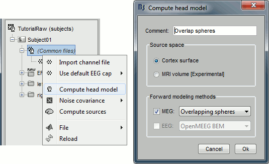
Right-click on the Right condition and select Compute head model. The Head modeler window will appear.
![[ATTACH] [ATTACH]](/moin_static1911/brainstorm1/img/attach.png) ---
--- ![[ATTACH] [ATTACH]](/moin_static1911/brainstorm1/img/attach.png)
- Set the options for your head model:
Source space: Cortex surface.
The MRI volume option will be introduced in an advanced tutorial: Volume source estimation.Forward modeling method: Single sphere.
You can also edit the Comment field of the file that will be created (the string that will be representing the head model in the database explorer).
Click on Run.
Two other windows appear, to help you define the sphere. Estimating the best fitting sphere for a head is not always as easy as it looks like, because a human head is usually not spherical.
![[ATTACH] [ATTACH]](/moin_static1911/brainstorm1/img/attach.png)
![[ATTACH] [ATTACH]](/moin_static1911/brainstorm1/img/attach.png)
- Read and follow the instructions in the help window.
Click on the Scalp button, move and resize the sphere manually, just to see how it works.
Click again on Scalp: here we will use directly the estimation of the sphere based on the vertices of the Scalp surface (a simple least-squares fitting using all the vertices of the surface).
For EEG 3-shell spheres models, you just estimate and manipulate the largest sphere (scalp), and then use the Edit properties... button in the toolbar to define the relative radii of the 2 other spheres, and their respective conductivities. This will be described in another tutorial.
Click on Ok, and wait for a few seconds.
A new file appeared just below the channel file, it represents the head model.
![[ATTACH] [ATTACH]](/moin_static1911/brainstorm1/img/attach.png)
- There is not much you can do with this file, as it is only a matrix that converts the cortical sources into MEG/EEG recordings, and we do not have any sources information yet.
- You may just check the sphere(s) that were used to compute the head model.
Overlapping spheres model
Let's compute a more advanced forward model. The overlapping spheres method is based on the estimation of a different sphere for each sensor. Instead of using only one sphere for the whole head, it estimates a sphere that fits locally the shape of the head in the surroundings of each sensor.
Right-click on Right condition and select Compute head model again.
Select the Overlapping spheres method and click on Run.
- This algorithm is supposed to use the inner skull surface from the subject, but we usually do not have this information. In this case, a pseudo-innerskull is reconstructed using a dilated version of the cortex envelope.
Right-click on the new head model > Check spheres. This window shows the spheres that were estimated. You can check them by following the indications written in green at the bottom of the window: use left/right arrows. At each step, the current sensor marker is displayed in red, and the sphere you see is its local estimation of the head shape.
- Compute a head model for the Left condition (Overlapping spheres).
Selection of a head model
We now have two head models in for our Subject01 / Right condition.
- You can have several head models computed for the same dataset, but it is not recommended as it might be difficult afterwards to know which one was used to compute the sources.
If you want to keep them anyway, you have to indicate which one is the default one. You do that by double-clicking on one of them (or right-click > set as default head model), and it is supposed to turn green. The head model displayed in green is the one that will be used for the following computation steps.
- For MEG, when it works properly, the overlapping spheres model usually gives better results than the single sphere one. In this particular case, it produces more focal results, so we are going to use it for the next steps.
- For EEG, always prefer the "OpenMEEG BEM" model.
Now to make things clearer: delete the Single sphere head model, and keep the Overlapping spheres.
Batching head model computation
You can run in two clicks the computation of the overlapping spheres model for all the conditions or subjects you want in the database.
The Compute head model menu is available in popup menus in the tree at all the levels (protocol, subject, condition). It is then applied recursively to all the subjects and conditions contained in the node(s) you selected.
Example: If you want to compute it on all the subjects and all the conditions, select the Compute head model menu from the protocol node TutorialCtf. For all the conditions of Subject01, run it from the Subject01 popup menu. Etc.
If you only want to compute it on some subjects of the protocol, select them at once holding the Ctrl key, right-click on one, and select the Compute head model menu.
To process all the subjects for one condition, switch to the Functional data (sorted by conditions) view of the database.
Additional discussions on the forum
Sensor modeling: http://neuroimage.usc.edu/forums/showthread.php?1295
Gain matrix: http://neuroimage.usc.edu/forums/showthread.php?918
EEG reference: http://neuroimage.usc.edu/forums/showthread.php?1525#post6718
EEG and default anatomy: http://neuroimage.usc.edu/forums/showthread.php?1774
Mixed head models indices: http://neuroimage.usc.edu/forums/showthread.php?1878
From continuous tutorials:
Source analysis
Let's reproduce the same observations at the source level. The concepts related with the source estimation are not discussed here; for more information, refer to the introduction tutorials #6 to #8.
First, delete all the files related with the source estimation calculated in the previous tutorials, available in the (Common files) folder: the head model, the noise covariance and inverse model. We can now provide a better estimate of the noise (affects the inverse model), and we defined new SSP operators (affects the head model).
Head model
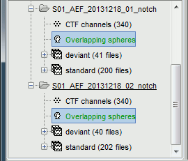
Right-click on any node that contains the channel file (including the channel file itself), and select: "Compute head model". Leave all the default options: cortex source space, and overlapping spheres. The lead field matrix is saved in file "Overlapping spheres" in (Common files).

From auditory
Head model
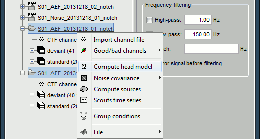
Select the two imported folders at once, right-click > Compute head model
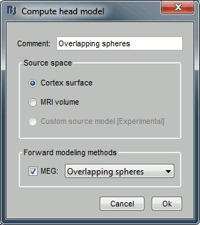
Use the overlapping spheres model and keep all of the options at their default values.
For more information: Head model tutorial.
What's in the headmodel file


