|
Size: 6032
Comment:
|
Size: 14023
Comment:
|
| Deletions are marked like this. | Additions are marked like this. |
| Line 4: | Line 4: |
| This tutorial explains how to use recordings from the CTF current phantom to test dipole fitting functions. | This tutorial explains how to import and process CTF current phantom recordings. We decided to release this example for testing and cross-validation purposes. With these datasets, we can evaluate the equivalence of various forward models and dipole fitting methods in the case of simple recordings with single dipoles. The recordings are available in two file formats (native and FIF) to cross-validate the file readers available in Brainstorm and MNE. A similar page exists for the [[Tutorials/PhantomElekta|Elekta-Neuromag phantom]]. |
| Line 8: | Line 8: |
| == Phantom description == '''[TODO]''' Pictures |
== License == This tutorial dataset remains a property of its authors: Elizabeth Bock, Francois Tadel and Sylvain Baillet (MEG Lab, McConnell Brain Imaging Center, Montreal Neurological Institute, McGill University, Canada). |
| Line 11: | Line 11: |
| '''[TODO]''' Nature of the dipole that is generated | If you reference this dataset in your publications, please aknowledge them and cite Brainstorm as indicated on the [[http://neuroimage.usc.edu/brainstorm/CiteBrainstorm|website]]. For questions, please contact us through the forum. |
| Line 13: | Line 13: |
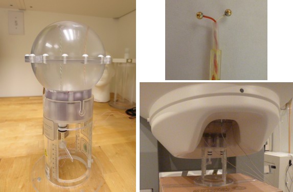
| '''[TODO]''' References | == CTF current phantom == The CTF current dipole phantom is a spherical container filled with a conducting saline solution which contains a current source and sink. This electric dipole is used to simulate brain sources in a conductive medium. The globe has a 130mm inner diameter and small attachment posts to attach the three CTF head localization coils. The position of this dipole can be adjusted within this globe. The dipole itself is constructed of two gold spheres about 2 mm in diameter, separated by 9.0 mm center to center. The dipole moment can be calculated by the equation '''m=I.L''', where I is the current flow (in Amperes) and L is the length of the dipole (0.009 meters). The location of the dipole is recorded relative to the center of the sphere (0,0,0)m, where X is positive toward the nasion, Y is positive toward the left ear and Z is positive toward the top of the head (see the [[CoordinateSystems]] tutorial for more details). . {{attachment:phantom_ctf.jpg}} ==== Reference ==== VSM/CTF documentation: PN900-0018, Revision 3.2, 23 November 2006. This document can be found with your full CTF installation at /opt/ctf/docs/Phantom.pdf. == Description of the experiment == Files distributed as part of the CTF phantom tutorial: * phantom_ctf/ds/phantom_200uA_20150709_01.ds<<BR>>Current='''200uA''', Moment='''1800nAm''', Frequency='''7Hz''', Location='''(0, -18, 49)mm''' - 03-Jul-2015 <<BR>>This corresponds to a very strong dipole, that could be studied without any averaging. * phantom_ctf/ds/phantom_20uA_20150603_03.ds<<BR>>Current='''20uA''', Moment='''180nAm''', Frequency='''23Hz''', Location='''(0, -18, 49)mm''' - 03-Jun-2015<<BR>>This is a weaker dipole, closer to the range of amplitudes we can except from the brain. You will not see the dipole activity emerging from the noise without averaging a few cycles together. * phantom_ctf/ds/emptyroom_20150709_01.ds<<BR>>MEG empty room measurements: the phantom is in the MEG helmet but not connected - 09-Jul-2015 * phantom_ctf/ds/phantom_20160222_01.pos<<BR>>"Head shape" of the phantom digitized with a Polhemus device using the [[Tutorials/TutDigitize|Brainstorm digitizer]]. * phantom_ctf/fif/phantom_20uA_20150603_03.fif<<BR>>Dataset 20uA converted to FIF format using MNE utility mne_ctf2fiff * phantom_ctf/fif/phantom_200uA_20150709_01.fif<<BR>>Dataset 200uA converted to FIF format using MNE utility mne_ctf2fiff * All recordings were performed by Elizabeth Bock at the MEG lab at McGill with a CTF MEG system with 275 axial gradiometers. |
| Line 16: | Line 37: |
| * '''Requirements''': You have already followed all the introduction tutorials and you have a working copy of Brainstorm installed on your computer. * Go to the [[http://neuroimage.usc.edu/brainstorm3_register/download.php|Download]] page of this website, and download the file: '''sample_phantom.zip''' |
* '''Requirements''': You have followed the introduction tutorials and Brainstorm is installed. * Go to the [[http://neuroimage.usc.edu/bst/download.php|Download]] page of this website, and download the file: '''sample_phantom_ctf.zip''' |
| Line 25: | Line 46: |
| * In the Matlab command window: type "'''generate_ctf_phantom'''". * This creates a new subject '''Phantom''' and generates the "anatomy" for this device: one volume and a few surfaces representing the geometry of the phantom. <<BR>><<BR>> {{attachment:phantom_anat.gif||height="178",width="208"}} |
* In the Matlab command window: type "'''generate_phantom''''''_ctf'''". * This creates a new subject '''PhantomCTF''' and generates the "anatomy" for this device: one volume and a few surfaces representing the geometry of the phantom. <<BR>><<BR>> {{attachment:phantom_anat.gif||height="178",width="208"}} |
| Line 31: | Line 52: |
| * Right-click on the subject folder > '''Review raw file'''. <<BR>>Select the file format: "'''MEG/EEG: CTF (*.ds)'''" <<BR>>Select all the folders in: '''sample_phantom'''. <<BR>><<BR>> {{attachment:phantom_review.gif||height="197",width="512"}} | * Right-click on the subject folder > '''Review raw file'''. <<BR>>Select the file format: "'''MEG/EEG: CTF (*.ds)'''" <<BR>>Select all the folders in: '''sample_phantom_ctf/ds'''. <<BR>><<BR>> {{attachment:phantom_review.gif||height="197",width="512"}} |
| Line 37: | Line 58: |
| * For each of the three runs: right-click on "Link to raw file" > '''Switch epoched/continuous''' <<BR>><<BR>> {{attachment:phantom_continuous.gif}} | * For each of the three runs: right-click on "Link to raw file" > '''Switch epoched/continuous''' <<BR>><<BR>> {{attachment:phantom_continuous.gif||height="163",width="255"}} |
| Line 40: | Line 61: |
| * Mark events: The sinusoidal signal is generated by the CTF hardware on channel HDAC006. While there are some automatic trigger events generated by the system that can be used for importing (event type HDAC006), we will have a more precise event average if the events are detected again offline. * Put the two phantom raw links in the Process1 box, click '''Run > Events > Detect events above threshold''': Event name=stim, Channel name=HDAC006, All file, Max thresh=0.5, units None, no filter, uncheck absolute value, check remove DC. * Then add the process '''Events > Convert to simple event''': Event names=stim, select Keep the middle of the events * Import the stim event: * Put the two phantom raw links in the Process1 box, click '''Run > Import recordings > Import MEG/EEG: Events''': Subject name=Phantom, Event names=stim, All file, Epoch time=[-70,70]ms, uncheck Create one condition, check the last three boxes * Add the process '''Pre-process > Remove DC offset''': All file, Sensor types=MEG, check overwrite * Add the process '''Average > Average files''': By trial group (folder average) |
==== Event detection ==== The sinusoidal signal is generated by the CTF hardware on channel HDAC006. While there are some automatic trigger events generated by the system that can be used for importing, we will have a more precise event average if the events are detected again offline. * In Process1: Select the 20uA and 200uA links, then click on [Run]. * Select process: '''Events > Detect events above threshold'''<<BR>>Event name='''stim''', Channel name='''HDAC006''', Time window='''[0,10]s''', Max thresh='''0.5''', Units='''None''', No filter, Uncheck absolute value, Check remove DC. <<BR>><<BR>> {{attachment:phantom_detect.gif||height="365",width="391"}} * Add the process '''Events > Convert to simple event''':<<BR>>Event names='''stim''', Keep the middle of the events. <<BR>><<BR>> {{attachment:phantom_detect2.gif||height="223",width="264"}} {{attachment:phantom_detect3.gif||height="172",width="385"}} ==== Import and average ==== * In Process1: Keep the same files selected (20uA and 200uA links), then click on [Run]. * Select process: '''Import recordings > Import MEG/EEG: Events''': <<BR>>Subject name='''PhantomCtf''', Event names='''stim''', Time window='''[0,10]s''', Epoch time='''[-70,70]ms''', <<BR>>Uncheck Create one condition, Check the last three boxes. * Add process '''Pre-process > Remove DC offset''': All file, Sensor types=MEG, check Overwrite. * Add process '''Average > Average files''': By folder (subject average). Run the pipeline.<<BR>><<BR>> {{attachment:phantom_import.gif||height="338",width="234"}} {{attachment:phantom_import2.gif||height="216",width="209"}} {{attachment:phantom_average.gif||height="374",width="213"}} |
| Line 49: | Line 76: |
| * Using the emptyroom recording * Right-click on the '''Link to raw file > Noise covariance > Compute from recordings''': Baseline=[0,998.3]ms, select Block by block, Full matrix * Right-click on the '''Noise covariance: MEG > Copy to other folders''' |
Use the empty room recordings. |
| Line 53: | Line 78: |
| == Source modeling == * Compute head model: for each phantom recording, right-click on the respective channel files > Compute head model: MRI volume, MEG method=Overlapping spheres, Regular grid (isotropic)=2mm * Compute sources: right click the head model > Compute sources [2015] > Dipole modeling, NP performance index * GLSp into Process1, Sources > Dipole scanning: All file |
* Right-click on the empty room '''Link to raw file > Noise covariance > Compute from recordings''': Baseline=[0,998.3]ms, select Block by block, Full matrix. <<BR>><<BR>> {{attachment:phantom_noisecov.gif||height="283",width="619"}} * Right-click on the '''Noise covariance: MEG > Copy to other folders'''. <<BR>><<BR>> {{attachment:phantom_noisecov2.gif||height="134",width="259"}} == Source estimation == Compute a forward model and inverse model for a regular grid inside the phantom volume. * In Process1, select the two averages (20uA and 200uA). <<BR>><<BR>> {{attachment:phantom_inverse3.gif||height="102",width="362"}} * Select process '''Sources > Compute head model''': MRI Volume, Regular grid (5mm), Single sphere.<<BR>>Increase the density of the grid for higher spatial accuracy.<<BR>><<BR>> {{attachment:phantom_headmodel1.gif||height="350",width="262"}} {{attachment:phantom_headmodel2.gif||height="350",width="266"}} * Add process '''Sources > Compute sources [2015]''': Kernel only (one per file), Dipole modeling. <<BR>><<BR>> {{attachment:phantom_inverse1.gif||height="250",width="298"}} {{attachment:phantom_inverse2.gif||height="322",width="227"}} == Dipole scanning == Scan the for the most significant dipole in the grid of computed dipoles estimate previously. * In Process1, select the source maps for the two conditions (20uA and 200uA)<<BR>>or leave the averaged recordings selected and click on [Process sources]. <<BR>><<BR>> {{attachment:phantom_dipscan.gif||height="109",width="365"}} * Run process '''Sources > Dipole scanning''': Time window='''[0,0]ms'''<<BR>><<BR>> {{attachment:phantom_dipscan2.gif||height="247",width="298"}} {{attachment:phantom_dipscan3.gif||height="242",width="282"}} * Right-click on the dipole file > '''File > View file contents''': <<BR>><<BR>> {{attachment:phantom_dipscan4.gif||height="232",width="471"}} * Note that there is no non-linear fitting in this process. This operation selects a dipole in the grid of points available in the grid with a 5mm spacing we used during the computation of the forward model. Therefore the localisation cannot be more precise than the resolution of the grid, all the results have to interpreted with an uncertainty of '''+/-2.5mm'''. * For a higher spatial resolution, you just need to recompute another forward model with a denser grid (2mm spacing for a 1mm precision). |
| Line 59: | Line 98: |
| Perform a non-linear dipole fit with the function ft_dipolefitting from the FieldTrip toolbox. * In Process1, select the average recordings for the two conditions (20uA and 200uA). * Run process '''Sources > FieldTrip: ft_dipolefitting''': Time window='''[0,0]''', Sensor type='''MEG'''<<BR>><<BR>> {{attachment:phantom_dipfit.gif||height="350",width="290"}} * Right-click on the dipole file > '''File > View file contents''': <<BR>><<BR>> {{attachment:phantom_dipfit2.gif||height="233",width="534"}} * The dipoles obtained with this non-linear dipole fitting method generally have a higher goodness of fit and a more accurate location than the dipole scanning previously illustrated. But this precision comes with computation costs that can be significantly higher in the case of more realistic head models. == Results comparison == ||<rowstyle="font-weight:bold;">Condition ||Method ||Forward model ||X ||Y ||Z ||GOF || || ||Nominal location || ||0 ||-18 ||49 ||mm || ||200uA ||Scanning (5mm) ||Single sphere ||-1.00 ||-16.00 ||44.00 ||99.80% || || ||Scanning (5mm) ||Overlapping spheres ||-1.00 ||-16.00 ||44.00 ||99.81% || || ||Scanning (5mm) ||OpenMEEG BEM ||-1.00 ||-16.00 ||44.00 ||99.76% || || ||Fitting ||Single sphere ||-1.04 ||-17.00 ||43.98 ||99.95% || || ||Fitting ||Overlapping spheres ||-1.05 ||-16.98 ||44.00 ||99.95% || || ||CTF software || ||-1 ||-17 ||44 ||99.95% || || ||MNE software || ||-0.79 ||-17.00 ||43.98 ||99.9% || || || || || || || || || ||20uA ||Scanning (5mm) ||Single sphere ||-1.00 ||-16.00 ||44.00 ||96.94% || || ||Scanning (5mm) ||Overlapping spheres ||-1.00 ||-16.00 ||44.00 ||96.96% || || ||Scanning (5mm) ||OpenMEEG BEM ||-1.00 ||-16.00 ||44.00 ||96.90% || || ||Fitting ||Single sphere ||-1.75 ||-17.13 ||44.39 ||98.25% || || ||Fitting ||Overlapping spheres ||-1.78 ||-17.14 ||44.45 ||98.25% || || ||CTF software || ||-1 ||-17 ||44 ||98.38% || || ||MNE software || ||-1.38 ||-16.31 ||44.01 ||99.1% || The nominal location indicates where the dipole is supposed to be, relative to the center of the sphere. It is measured with rulers with an overall precision of about 5mm. The range of discrepancy we observe between this nominal location and the position of the dipole estimated from the recordings is acceptable. |
|
| Line 64: | Line 132: |
| For additional testing purposes, the .pos file for the phantom is included in the sample_phantom.zip package, but you have to add it manually to the recordings. Do not use these points to refine automatically the registration: the fitting algorithm may fail finding the best rotation around the Z axis because the phantom is completely spherical, and the registration is already close to perfection. | For additional testing purposes, the .pos file for the phantom is included in the sample_phantom_ctf.zip package, but you have to add it manually to the recordings. Do not use these points to refine automatically the registration: the fitting algorithm may fail finding the best rotation around the Z axis because the phantom is completely spherical, and the registration is already close to perfection. |
| Line 66: | Line 134: |
| * Right-click on one of the channel files (20uA or 200uA) > '''Digitized head points > Add points'''.<<BR>>Select the file format: "'''EEG: Polhemus'''"<<BR>>Select file: sample_phantom/'''phantom_20160222_01.pos'''<<BR>><<BR>><<BR>> {{attachment:phantom_pos.gif||height="165",width="608"}} | * Right-click on one of the channel files (20uA or 200uA) > '''Digitized head points > Add points'''.<<BR>>Select the file format: "'''EEG: Polhemus'''"<<BR>>Select file: sample_phantom_ctf/ds/'''phantom_20160222_01.pos'''<<BR>><<BR>><<BR>> {{attachment:phantom_pos.gif||height="165",width="608"}} |
| Line 71: | Line 139: |
| Available in the Brainstorm distribution: '''brainstorm3/toolbox/script/tutorial_phantom.m ''' | Available in the Brainstorm distribution: '''brainstorm3/toolbox/script/tutorial_phantom_ctf.m''' |
MEG current phantom (CTF)
Authors: Francois Tadel, Elizabeth Bock
This tutorial explains how to import and process CTF current phantom recordings. We decided to release this example for testing and cross-validation purposes. With these datasets, we can evaluate the equivalence of various forward models and dipole fitting methods in the case of simple recordings with single dipoles. The recordings are available in two file formats (native and FIF) to cross-validate the file readers available in Brainstorm and MNE. A similar page exists for the Elekta-Neuromag phantom.
Contents
License
This tutorial dataset remains a property of its authors: Elizabeth Bock, Francois Tadel and Sylvain Baillet (MEG Lab, McConnell Brain Imaging Center, Montreal Neurological Institute, McGill University, Canada).
If you reference this dataset in your publications, please aknowledge them and cite Brainstorm as indicated on the website. For questions, please contact us through the forum.
CTF current phantom
The CTF current dipole phantom is a spherical container filled with a conducting saline solution which contains a current source and sink. This electric dipole is used to simulate brain sources in a conductive medium. The globe has a 130mm inner diameter and small attachment posts to attach the three CTF head localization coils. The position of this dipole can be adjusted within this globe.
The dipole itself is constructed of two gold spheres about 2 mm in diameter, separated by 9.0 mm center to center. The dipole moment can be calculated by the equation m=I.L, where I is the current flow (in Amperes) and L is the length of the dipole (0.009 meters).
The location of the dipole is recorded relative to the center of the sphere (0,0,0)m, where X is positive toward the nasion, Y is positive toward the left ear and Z is positive toward the top of the head (see the CoordinateSystems tutorial for more details).
Reference
VSM/CTF documentation: PN900-0018, Revision 3.2, 23 November 2006. This document can be found with your full CTF installation at /opt/ctf/docs/Phantom.pdf.
Description of the experiment
Files distributed as part of the CTF phantom tutorial:
phantom_ctf/ds/phantom_200uA_20150709_01.ds
Current=200uA, Moment=1800nAm, Frequency=7Hz, Location=(0, -18, 49)mm - 03-Jul-2015
This corresponds to a very strong dipole, that could be studied without any averaging.phantom_ctf/ds/phantom_20uA_20150603_03.ds
Current=20uA, Moment=180nAm, Frequency=23Hz, Location=(0, -18, 49)mm - 03-Jun-2015
This is a weaker dipole, closer to the range of amplitudes we can except from the brain. You will not see the dipole activity emerging from the noise without averaging a few cycles together.phantom_ctf/ds/emptyroom_20150709_01.ds
MEG empty room measurements: the phantom is in the MEG helmet but not connected - 09-Jul-2015phantom_ctf/ds/phantom_20160222_01.pos
"Head shape" of the phantom digitized with a Polhemus device using the Brainstorm digitizer.phantom_ctf/fif/phantom_20uA_20150603_03.fif
Dataset 20uA converted to FIF format using MNE utility mne_ctf2fiffphantom_ctf/fif/phantom_200uA_20150709_01.fif
Dataset 200uA converted to FIF format using MNE utility mne_ctf2fiffAll recordings were performed by Elizabeth Bock at the MEG lab at McGill with a CTF MEG system with 275 axial gradiometers.
Download and installation
Requirements: You have followed the introduction tutorials and Brainstorm is installed.
Go to the Download page of this website, and download the file: sample_phantom_ctf.zip
- Unzip it in a folder that is not in any of the Brainstorm folders (program folder or database folder)
- Start Brainstorm (Matlab scripts or stand-alone version)
Select the menu File > Create new protocol. Name it "TutorialPhantom" and select the options:
"No, use individual anatomy",
"No, use one channel file per acquisition run (MEG)".
Generate anatomy
In the Matlab command window: type "generate_phantom_ctf".
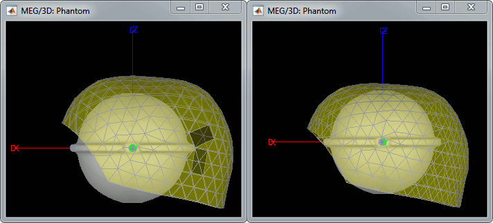
This creates a new subject PhantomCTF and generates the "anatomy" for this device: one volume and a few surfaces representing the geometry of the phantom.
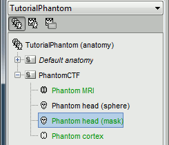
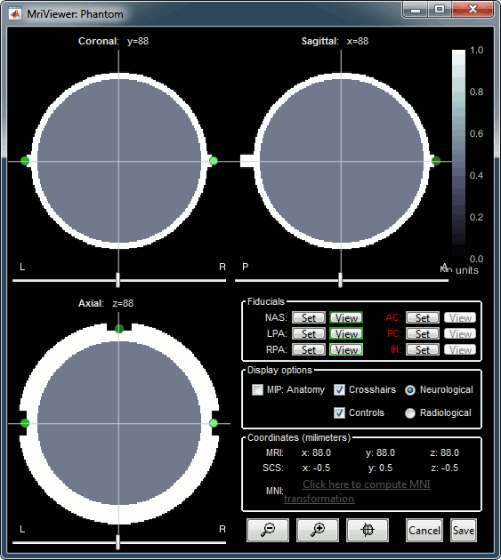
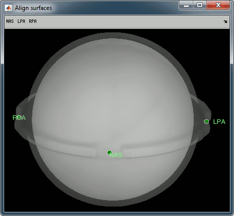
You can display the MRI and surfaces as presented in the introduction tutorials.
Access the recordings
- Switch to the "functional data" view.
Right-click on the subject folder > Review raw file.
Select the file format: "MEG/EEG: CTF (*.ds)"
Select all the folders in: sample_phantom_ctf/ds.
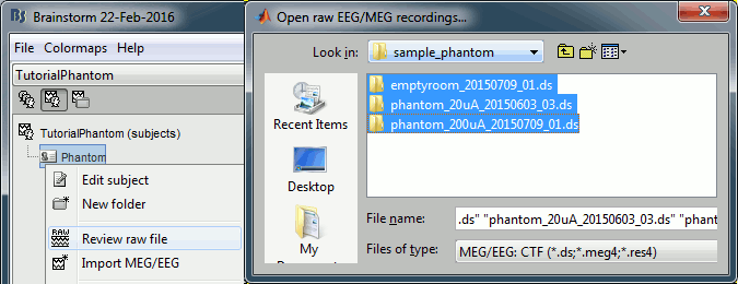
- Each folder corresponds to one dataset:
emptyroom_20150709_01.ds: Phantom inside the MEG helmet, but not plugged in
phantom_20uA_20150603_03.ds: Phantom active, 23Hz, 20uA, [0,-1.8,4.9]cm
phantom_200uA_20150709_01.ds: Phantom active, 7Hz, 200uA, [0,-1.8,4.9]cm
The recordings were acquired on different days, the position of the phantom in the MEG helmet is not the same for the two runs. Left = 20uA, Right = 200uA
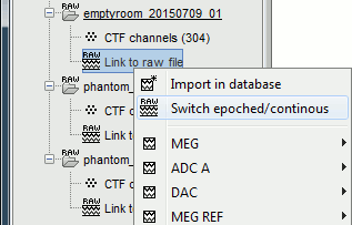
For each of the three runs: right-click on "Link to raw file" > Switch epoched/continuous
Import recordings
Event detection
The sinusoidal signal is generated by the CTF hardware on channel HDAC006. While there are some automatic trigger events generated by the system that can be used for importing, we will have a more precise event average if the events are detected again offline.
- In Process1: Select the 20uA and 200uA links, then click on [Run].
Select process: Events > Detect events above threshold
Event name=stim, Channel name=HDAC006, Time window=[0,10]s, Max thresh=0.5, Units=None, No filter, Uncheck absolute value, Check remove DC.
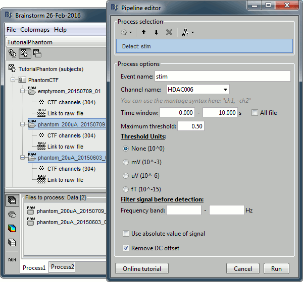
Add the process Events > Convert to simple event:
Event names=stim, Keep the middle of the events.
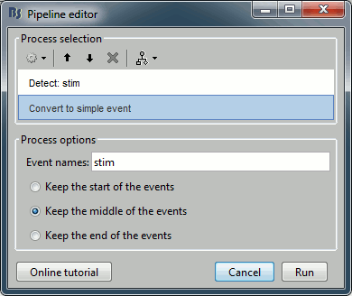
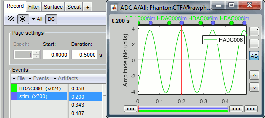
Import and average
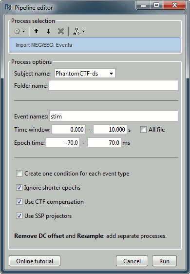
- In Process1: Keep the same files selected (20uA and 200uA links), then click on [Run].
Select process: Import recordings > Import MEG/EEG: Events:
Subject name=PhantomCtf, Event names=stim, Time window=[0,10]s, Epoch time=[-70,70]ms,
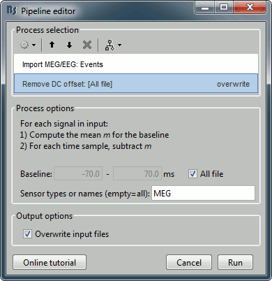
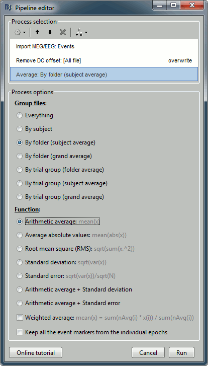
Uncheck Create one condition, Check the last three boxes.Add process Pre-process > Remove DC offset: All file, Sensor types=MEG, check Overwrite.
Add process Average > Average files: By folder (subject average). Run the pipeline.
Noise covariance
Use the empty room recordings.
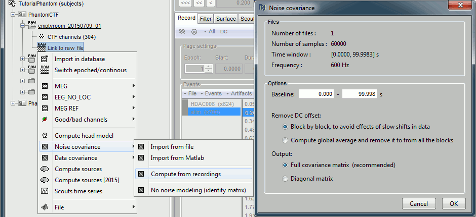
Right-click on the empty room Link to raw file > Noise covariance > Compute from recordings: Baseline=[0,998.3]ms, select Block by block, Full matrix.
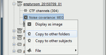
Right-click on the Noise covariance: MEG > Copy to other folders.
Source estimation
Compute a forward model and inverse model for a regular grid inside the phantom volume.
In Process1, select the two averages (20uA and 200uA).

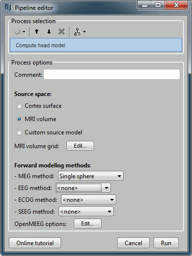
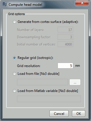
Select process Sources > Compute head model: MRI Volume, Regular grid (5mm), Single sphere.
Increase the density of the grid for higher spatial accuracy.
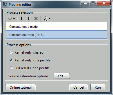
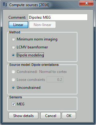
Add process Sources > Compute sources [2015]: Kernel only (one per file), Dipole modeling.
Dipole scanning
Scan the for the most significant dipole in the grid of computed dipoles estimate previously.
In Process1, select the source maps for the two conditions (20uA and 200uA)
or leave the averaged recordings selected and click on [Process sources].

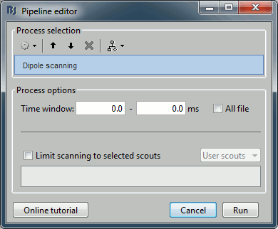
Run process Sources > Dipole scanning: Time window=[0,0]ms
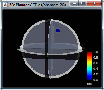
Right-click on the dipole file > File > View file contents:
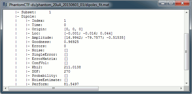
Note that there is no non-linear fitting in this process. This operation selects a dipole in the grid of points available in the grid with a 5mm spacing we used during the computation of the forward model. Therefore the localisation cannot be more precise than the resolution of the grid, all the results have to interpreted with an uncertainty of +/-2.5mm.
- For a higher spatial resolution, you just need to recompute another forward model with a denser grid (2mm spacing for a 1mm precision).
Dipole fitting with FieldTrip
Perform a non-linear dipole fit with the function ft_dipolefitting from the FieldTrip toolbox.
- In Process1, select the average recordings for the two conditions (20uA and 200uA).
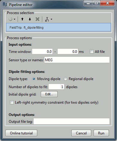
Run process Sources > FieldTrip: ft_dipolefitting: Time window=[0,0], Sensor type=MEG
Right-click on the dipole file > File > View file contents:
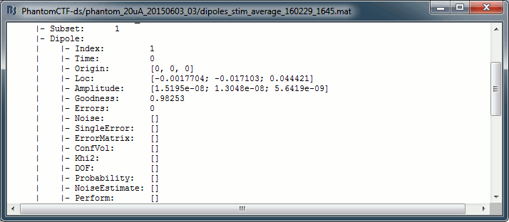
- The dipoles obtained with this non-linear dipole fitting method generally have a higher goodness of fit and a more accurate location than the dipole scanning previously illustrated. But this precision comes with computation costs that can be significantly higher in the case of more realistic head models.
Results comparison
Condition |
Method |
Forward model |
X |
Y |
Z |
GOF |
|
Nominal location |
|
0 |
-18 |
49 |
mm |
200uA |
Scanning (5mm) |
Single sphere |
-1.00 |
-16.00 |
44.00 |
99.80% |
|
Scanning (5mm) |
Overlapping spheres |
-1.00 |
-16.00 |
44.00 |
99.81% |
|
Scanning (5mm) |
OpenMEEG BEM |
-1.00 |
-16.00 |
44.00 |
99.76% |
|
Fitting |
Single sphere |
-1.04 |
-17.00 |
43.98 |
99.95% |
|
Fitting |
Overlapping spheres |
-1.05 |
-16.98 |
44.00 |
99.95% |
|
CTF software |
|
-1 |
-17 |
44 |
99.95% |
|
MNE software |
|
-0.79 |
-17.00 |
43.98 |
99.9% |
|
|
|
|
|
|
|
20uA |
Scanning (5mm) |
Single sphere |
-1.00 |
-16.00 |
44.00 |
96.94% |
|
Scanning (5mm) |
Overlapping spheres |
-1.00 |
-16.00 |
44.00 |
96.96% |
|
Scanning (5mm) |
OpenMEEG BEM |
-1.00 |
-16.00 |
44.00 |
96.90% |
|
Fitting |
Single sphere |
-1.75 |
-17.13 |
44.39 |
98.25% |
|
Fitting |
Overlapping spheres |
-1.78 |
-17.14 |
44.45 |
98.25% |
|
CTF software |
|
-1 |
-17 |
44 |
98.38% |
|
MNE software |
|
-1.38 |
-16.31 |
44.01 |
99.1% |
The nominal location indicates where the dipole is supposed to be, relative to the center of the sphere. It is measured with rulers with an overall precision of about 5mm. The range of discrepancy we observe between this nominal location and the position of the dipole estimated from the recordings is acceptable.
Digitized head points
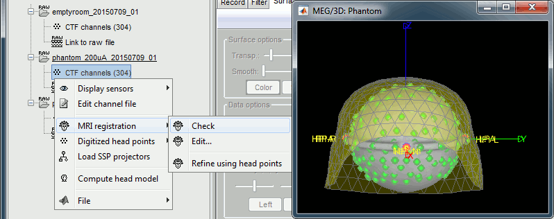
The head points collected with the Brainstorm digitizer are usually copied to the .ds folders and imported automatically when loading the recordings. We decided not to include them in this example because in the case of this current phantom, there is no ambiguity in the definition of the anatomical fiducials. As this refined registration with the .pos files is not part of the standard CTF workflow, not including it will make it easier to compare the workflow and results with other programs.
For additional testing purposes, the .pos file for the phantom is included in the sample_phantom_ctf.zip package, but you have to add it manually to the recordings. Do not use these points to refine automatically the registration: the fitting algorithm may fail finding the best rotation around the Z axis because the phantom is completely spherical, and the registration is already close to perfection.
Right-click on one of the channel files (20uA or 200uA) > Digitized head points > Add points.
Select the file format: "EEG: Polhemus"
Select file: sample_phantom_ctf/ds/phantom_20160222_01.pos

Right-click on the channel file > MRI registration > Check.
Scripting
Generate Matlab script
Available in the Brainstorm distribution: brainstorm3/toolbox/script/tutorial_phantom_ctf.m

