|
Size: 13987
Comment:
|
Size: 20147
Comment:
|
| Deletions are marked like this. | Additions are marked like this. |
| Line 4: | Line 4: |
| This tutorial explains how to import and process CTF current phantom recordings. We decided to release this example for testing and cross-validation purposes. With these datasets, we can evaluate the equivalence of various forward models and dipole fitting methods in the case of simple recordings with single dipoles. The recordings are available in two file formats (native and FIF) to cross-validate the file readers available in Brainstorm and MNE. A similar page exists for the [[Tutorials/PhantomCtf|CTF phantom]]. | This tutorial explains how to import and process Elekta-Neuromag current phantom recordings. We decided to release this example for testing and cross-validation purposes. With these datasets, we can evaluate the equivalence of various forward models and dipole fitting methods in the case of simple recordings with single dipoles. The recordings are available in two file formats (native and FIF) to cross-validate the file readers available in Brainstorm and MNE. A similar page exists for the [[Tutorials/PhantomCtf|CTF phantom]]. |
| Line 9: | Line 9: |
| This tutorial dataset remains a property of its authors. If you reference this dataset in your publications, please aknowledge them and cite Brainstorm as indicated on the [[http://neuroimage.usc.edu/brainstorm/CiteBrainstorm|website]]. For questions, please contact us through the forum. '''Neuromag phantom'''<<BR>>Authors: John Mosher<<BR>>Epilepsy Center, Cleveland Clinic Neurological Institute, Cleveland, OH USA. == CTF current phantom == The CTF current dipole phantom is a spherical container filled with a conducting saline solution which contains a current source and sink. This electric dipole is used to simulate brain sources in a conductive medium. The globe has a 130mm inner diameter and small attachment posts to attach the three CTF head localization coils. The position of this dipole can be adjusted within this globe. The dipole itself is constructed of two gold spheres about 2 mm in diameter, separated by 9.0 mm center to center. The dipole moment can be calculated by the equation '''m=I.L''', where I is the current flow (in Amperes) and L is the length of the dipole (0.009 meters). The location of the dipole is recorded relative to the center of the sphere (0,0,0)m, where X is positive toward the nasion, Y is positive toward the left ear and Z is positive toward the top of the head (see the [[CoordinateSystems]] tutorial for more details). . {{attachment:phantom_ctf.jpg}} ==== Reference ==== VSM/CTF documentation: PN900-0018, Revision 3.2, 23 November 2006. This document can be found with your full CTF installation at /opt/ctf/docs/Phantom.pdf. |
This tutorial dataset remains a property of its authors: Ken Taylor, John Mosher (Epilepsy Center, Cleveland Clinic Neurological Institute, Cleveland, OH USA). If you reference this dataset in your publications, please acknowledge them and cite Brainstorm as indicated on the [[http://neuroimage.usc.edu/brainstorm/CiteBrainstorm|website]]. For questions, please contact us through the forum. == The phantom == A current phantom is provided with the Elekta Neuromag for checking the system performance. It contains 32 artificial dipoles and four fixed head-position indicator coils. The phantom is based on the mathematical fact that an equilateral triangular line current produces equivalent magnetic field distribution to that of a tangential current dipole in a spherical conductor, provided that the vertex of the triangle and the origin of the conducting sphere coincide. For a detailed description of how the phantom works, see [[http://neuroimage.usc.edu/paperspdf/1985_IlmoniemHamKnuu_ForwardInversModel.pdf|here]]. The phantom dipoles are energized using an internal signal generator which also feeds the HPI coils. An external multiplexer box is used to connect the signal to the individual dipoles. Only one dipole can be activated at a time. The location of the dipole is recorded relative to the center of the sphere (0,0,0)m, where X is positive toward the nasion, Y is positive toward the left ear and Z is positive toward the top of the head (see the [[CoordinateSystems]] tutorial for more details). Use of the phantom is shown below. Note that the uncovered version is the phantom that came with the Neuromag-122, which explicitly shows the wiring. The covered version uses the same principle but somewhat different dipole locations. Further details are available in Section 7.2 of the User's Manual. . {{attachment:phantom.gif||height="366",width="632"}} ==== References ==== * R.J. Ilmoniemi, M.S. Hämäläinen, and J. Knuutila, The Forward and Inverse Problems in the Spherical Model. In: Biomagnetism: Applications and Theory, eds. H. Weinberg, G. Stroink, T. Katil, Pergamon Press, 1985. * Elekta Neuromag System Hardware User's Manual, Revision G, September 2005. |
| Line 26: | Line 27: |
| Files distributed as part of the CTF phantom tutorial: * phantom_ctf/ds/phantom_200uA_20150709_01.ds<<BR>>Current='''200uA''', Moment='''1800nAm''', Frequency='''7Hz''', Location='''(0, -18, 49)mm''' - 03-Jul-2015 <<BR>>This corresponds to a very strong dipole, that could be studied without any averaging. * phantom_ctf/ds/phantom_20uA_20150603_03.ds<<BR>>Current='''20uA''', Moment='''180nAm''', Frequency='''23Hz''', Location='''(0, -18, 49)mm''' - 03-Jun-2015<<BR>>This is a weaker dipole, closer to the range of amplitudes we can except from the brain. You will not see the dipole activity emerging from the noise without averaging a few cycles together. * phantom_ctf/ds/emptyroom_20150709_01.ds<<BR>>MEG empty room measurements: the phantom is in the MEG helmet but not connected - 09-Jul-2015 * phantom_ctf/ds/phantom_20160222_01.pos<<BR>>"Head shape" of the phantom digitized with a Polhemus device using the [[Tutorials/TutDigitize|Brainstorm digitizer]]. * phantom_ctf/fif/phantom_20uA_20150603_03.fif<<BR>>Dataset 20uA converted to FIF format using MNE utility mne_ctf2fiff * phantom_ctf/fif/phantom_200uA_20150709_01.fif<<BR>>Dataset 200uA converted to FIF format using MNE utility mne_ctf2fiff * All recordings were performed by Elizabeth Bock at the MEG lab at McGill with a CTF MEG system with 275 axial gradiometers. |
Files distributed as part of the phantom Elekta tutorial: * kojak_all_2000nAm_pp_no_chpi_no_ms_raw.fif<<BR>>Source =''' 2000 nAm'''. This corresponds to an unrealistically strong 1,000 nA-m (2,000 nA-m peak to peak) dipole that gives the highest SNR visualization of the experimental source. * kojak_all_200nAm_pp_no_chpi_no_ms_raw.fif<<BR>>Source =''' 200 nAm'''. This is a weaker dipole, closer to the range of amplitudes we can expect from inter-ictal spikes due to epilepsy, visible in raw data. * kojak_all_20nAm_pp_no_chpi_no_ms_raw.fif<<BR>>Source =''' 20 nAm'''. This represents some of the weakest sources we expect in evoked studies which require averaging to detect and estimate (i.e. generally cannot be seen in single trials). * All recordings were performed by John Mosher in the MEG lab at the Cleveland Clinic with an Elekta phantom. |
| Line 38: | Line 36: |
| * Go to the [[http://neuroimage.usc.edu/bst/download.php|Download]] page of this website, and download the file: '''sample_phantom.zip''' | * Go to the [[http://neuroimage.usc.edu/bst/download.php|Download]] page and download the file: '''sample_phantom_elekta.zip''' |
| Line 41: | Line 39: |
| * Select the menu File > Create new protocol. Name it "'''TutorialPhantom'''" and select the options: * "'''No, use individual anatomy'''", * "'''No, use one channel file per acquisition run (MEG)'''". |
* Select the menu File > Create new protocol. Name it '''TutorialPhantomElekta''' and select: * '''No, use individual anatomy''', * '''No, use one channel file per acquisition run (MEG)'''. |
| Line 46: | Line 44: |
| * In the Matlab command window: type "'''generate_phantom''''''_ctf'''". * This creates a new subject '''PhantomCTF''' and generates the "anatomy" for this device: one volume and a few surfaces representing the geometry of the phantom. <<BR>><<BR>> {{attachment:phantom_anat.gif||height="178",width="208"}} * You can display the MRI and surfaces as presented in the introduction tutorials. <<BR>><<BR>> {{attachment:phantom_mri.gif||height="314",width="281"}} {{attachment:phantom_surfaces.gif||height="314",width="341"}} |
* In the Matlab command window: type "'''generate_phantom''''''_elekta'''". * This creates a new subject '''Kojak''' (so named after the 70's TV show) and generates the "anatomy" for this device: one volume and a few surfaces representing the geometry of the phantom. <<BR>><<BR>> . {{attachment:kojak_anat.gif||height="247",width="630"}} <<BR>><<BR>> * You can display the MRI and surfaces as presented in the introduction tutorials. <<BR>><<BR>> {{attachment:phantom_mri.gif}} {{attachment:phantom_surfaces.gif}} |
| Line 51: | Line 52: |
| * Switch to the "functional data" view. * Right-click on the subject folder > '''Review raw file'''. <<BR>>Select the file format: "'''MEG/EEG: CTF (*.ds)'''" <<BR>>Select all the folders in: '''sample_phantom/phantom_ctf/ds'''. <<BR>><<BR>> {{attachment:phantom_review.gif||height="197",width="512"}} * Each folder corresponds to one dataset: * '''emptyroom_20150709_01.ds''': Phantom inside the MEG helmet, but not plugged in * '''phantom_20uA_20150603_03.ds''': Phantom active, 23Hz, 20uA, [0,-1.8,4.9]cm * '''phantom_200uA_20150709_01.ds''': Phantom active, 7Hz, 200uA, [0,-1.8,4.9]cm * The recordings were acquired on different days, the position of the phantom in the MEG helmet is not the same for the two runs. Left = 20uA, Right = 200uA<<BR>><<BR>> {{attachment:phantom_registration.gif||height="189",width="417"}} * For each of the three runs: right-click on "Link to raw file" > '''Switch epoched/continuous''' <<BR>><<BR>> {{attachment:phantom_continuous.gif||height="163",width="255"}} == Import recordings == ==== Event detection ==== The sinusoidal signal is generated by the CTF hardware on channel HDAC006. While there are some automatic trigger events generated by the system that can be used for importing, we will have a more precise event average if the events are detected again offline. * In Process1: Select the 20uA and 200uA links, then click on [Run]. * Select process: '''Events > Detect events above threshold'''<<BR>>Event name='''stim''', Channel name='''HDAC006''', Time window='''[0,10]s''', Max thresh='''0.5''', Units='''None''', No filter, Uncheck absolute value, Check remove DC. <<BR>><<BR>> {{attachment:phantom_detect.gif||height="365",width="391"}} * Add the process '''Events > Convert to simple event''':<<BR>>Event names='''stim''', Keep the middle of the events. <<BR>><<BR>> {{attachment:phantom_detect2.gif||height="223",width="264"}} {{attachment:phantom_detect3.gif||height="172",width="385"}} ==== Import and average ==== * In Process1: Keep the same files selected (20uA and 200uA links), then click on [Run]. * Select process: '''Import recordings > Import MEG/EEG: Events''': <<BR>>Subject name='''PhantomCtf''', Event names='''stim''', Time window='''[0,10]s''', Epoch time='''[-70,70]ms''', <<BR>>Uncheck Create one condition, Check the last three boxes. * Add process '''Pre-process > Remove DC offset''': All file, Sensor types=MEG, check Overwrite. * Add process '''Average > Average files''': By folder (subject average). Run the pipeline.<<BR>><<BR>> {{attachment:phantom_import.gif||height="338",width="234"}} {{attachment:phantom_import2.gif||height="216",width="209"}} {{attachment:phantom_average.gif||height="374",width="213"}} |
We can now review one of the raw kojak data sets. These have been generated by sequentially activating each of the 32 phantom dipoles in a single raw file. * Switch to the '''functional data''' view by clicking the second button under the protocol name. * Right-click on the subject folder > '''Review raw file'''. * Select the '''200nA''' source. * Click '''Event channel''', select '''STI201''', and hit '''OK'''. Close the figure and double click the link to raw file to open a list of the events. At this point, you may wish to rename your groups so that the ordering remains convenient. To do this, click group 1, click '''Events''' > '''Rename group''', and rename it to '''01'''. Repeat this for 2 - 9. This step, and others like it, can also be performed by importing the data into '''MATLAB''', running the following code below, and then exporting the data back into Brainstorm: {{{ % to change the trigger numbers to appear sequentially for i = 1:32, STR = str2num(link_filename.F.events(i).label); link_filename.F.events(i).label = sprintf('%02.0f',STR); end }}} Some other triggers are generated by the neuromag system which are unnecessary so we will delete them: * Trim away the singleton events by clicking on '''256 (x1)''', shift clicking on '''7936 (x1)''' and pressing the '''delete''' key. There is also a switching transient in the phantom generator which should be removed: * Remove the first event from dipole '''01''' by clicking on it, clicking on the '''first''' time instant, and pressing the '''delete''' key. Events should now appear as per the image below on the right: <<BR>> . {{attachment:editing_events.gif||height="444",width="630"}} __'''Note:'''__''' '''Make sure to save the modifications that you make before proceeding. If you hit the grey X to close all figures and clear memory, you will be prompted to save modifications, and you should click '''Yes'''. == Importing the dipole events == Right click on '''Link to raw file''' and click '''Import in database''' * Uncheck '''Apply SSP/ICA projectors''' (we will use noise covariance to stabilize the data) * Check '''Remove DC offset''', set the time range from -100 to -10ms * Resample the recordings to '''100Hz''' (change from 1000Hz) * Do __not__ create separate folders * Click '''Import'''<<BR>><<BR>> {{attachment:kojak_dipole_import.gif||height="306",width="630"}} <<BR>><<BR>> |
| Line 76: | Line 97: |
| Use the empty room recordings. * Right-click on the empty room '''Link to raw file > Noise covariance > Compute from recordings''': Baseline=[0,998.3]ms, select Block by block, Full matrix. <<BR>><<BR>> {{attachment:phantom_noisecov.gif||height="283",width="619"}} * Right-click on the '''Noise covariance: MEG > Copy to other folders'''. <<BR>><<BR>> {{attachment:phantom_noisecov2.gif||height="134",width="259"}} == Source estimation == Compute a forward model and inverse model for a regular grid inside the phantom volume. * In Process1, select the two averages (20uA and 200uA). <<BR>><<BR>> {{attachment:phantom_inverse3.gif||height="102",width="362"}} * Select process '''Sources > Compute head model''': MRI Volume, Regular grid (5mm), Single sphere.<<BR>>Increase the density of the grid for higher spatial accuracy.<<BR>><<BR>> {{attachment:phantom_headmodel1.gif||height="350",width="262"}} {{attachment:phantom_headmodel2.gif||height="350",width="266"}} * Add process '''Sources > Compute sources [2015]''': Kernel only (one per file), Dipole modeling. <<BR>><<BR>> {{attachment:phantom_inverse1.gif||height="250",width="298"}} {{attachment:phantom_inverse2.gif||height="322",width="227"}} |
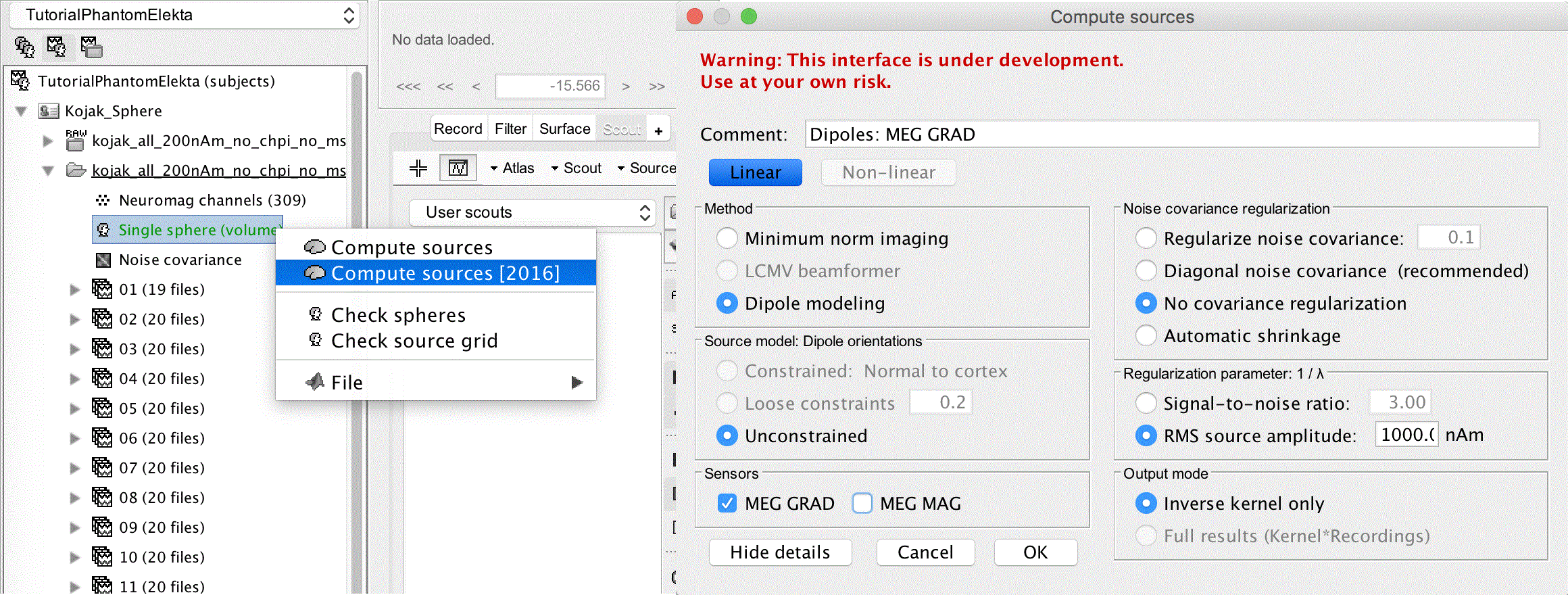
With the epochs loaded, we can now calculate the noise covariance from the prestims. To do this, '''select all 32 dipoles''' (click the first then shift click the last), then right click, '''Noise covariance''' > '''Compute from recordings'''. Uncheck '''MEG MAG''' and hit '''OK'''. <<BR>><<BR>> . {{attachment:kojak_noise_covariance.gif||height="216",width="630"}} <<BR>><<BR>> Average all of the epochs by '''selecting all 32 '''again, dragging them to the process box, clicking '''RUN'''. Next click the cog, and select '''Average''' > '''Average files'''. Group the files '''By trial group (folder average)''', and select '''Arithmetic average: mean(x)''', and click "'''Run'''". <<BR>><<BR>> . {{attachment:kojak_average.gif||height="420",width="630"}} == Head modelling == To compute the head model, right click on the '''kojak_all_200nA '''file and select '''Compute head model'''. * Source space: select '''MRI volume''' * Forward modeling methods: '''Single sphere'''<<BR>><<BR>> {{attachment:kojak_head_model.gif||height="233",width="630"}} . <<BR>> A figure opens showing a sphere fit to the phantom, however we can see that the location is a little off. In this case we alread know where the center of the sphere should be, so we adjust it manually: * Click the '''Edit sphere properties''' button in the top toolbar. * Change the center location to '''[ 0 0 0 ] '''and hit OK. The center of the sphere shifts to the correct position. Click the '''OK '''button next to the edit sphere properties button to perform the MRI/surface interpolation. A window appears allowing adjustment of the volume source grid. * Select '''Regular grid (isotropic) '''with '''Grid resolution 2.5mm''' This results in an around 56K grid point, which is sufficient.<<BR>><<BR>> . {{attachment:kojak_sphere.gif||height="335",width="630"}} . <<BR>> == Dipole source estimation == * Right click the Single sphere (volume) and select '''Compute sources [2016] ''' * Method: '''Dipole modeling''' * Source model: Dipole orientations '''Unconstrained''' For the sensor selection you can choose to use either the gradiometers or the magnetometers, in this case we select '''both'''. Click '''Show details '''if the noise covariance regularization is hidden. * Select '''Regularize noise covariance: 0.1''' * Ignore the other settings, and click '''OK'''<<BR>><<BR>> . {{attachment:kojak_compute_sources.gif||height="239",width="630"}} . <<BR>> |
| Line 89: | Line 145: |
| Scan the for the most significant dipole in the grid of computed dipoles estimate previously. * In Process1, select the source maps for the two conditions (20uA and 200uA)<<BR>>or leave the averaged recordings selected and click on [Process sources]. <<BR>><<BR>> {{attachment:phantom_dipscan.gif||height="109",width="365"}} * Run process '''Sources > Dipole scanning''': Time window='''[0,0]ms'''<<BR>><<BR>> {{attachment:phantom_dipscan2.gif||height="247",width="298"}} {{attachment:phantom_dipscan3.gif||height="242",width="282"}} * Right-click on the dipole file > '''File > View file contents''': <<BR>><<BR>> {{attachment:phantom_dipscan4.gif||height="232",width="471"}} * Note that there is no non-linear fitting in this process. This operation selects a dipole in the grid of points available in the grid with a 5mm spacing we used during the computation of the forward model. Therefore the localisation cannot be more precise than the resolution of the grid, all the results have to interpreted with an uncertainty of '''+/-2.5mm'''. * For a higher spatial resolution, you just need to recompute another forward model with a denser grid (2mm spacing for a 1mm precision). == Dipole fitting with FieldTrip == Perform a non-linear dipole fit with the function ft_dipolefitting from the FieldTrip toolbox. * In Process1, select the average recordings for the two conditions (20uA and 200uA). * Run process '''Sources > FieldTrip: ft_dipolefitting''': Time window='''[0,0]''', Sensor type='''MEG'''<<BR>><<BR>> {{attachment:phantom_dipfit.gif||height="350",width="290"}} * Right-click on the dipole file > '''File > View file contents''': <<BR>><<BR>> {{attachment:phantom_dipfit2.gif||height="233",width="534"}} * The dipoles obtained with this non-linear dipole fitting method generally have a higher goodness of fit and a more accurate location than the dipole scanning previously illustrated. But this precision comes with computation costs that can be significantly higher in the case of more realistic head models. == Results comparison == ||<rowstyle="font-weight:bold;">Condition ||Method ||Forward model ||X ||Y ||Z ||GOF || || ||Nominal location || ||0 ||-18 ||49 ||mm || ||200uA ||Scanning (5mm) ||Single sphere ||-1.00 ||-16.00 ||44.00 ||99.80% || || ||Scanning (5mm) ||Overlapping spheres ||-1.00 ||-16.00 ||44.00 ||99.81% || || ||Scanning (5mm) ||OpenMEEG BEM ||-1.00 ||-16.00 ||44.00 ||99.76% || || ||Fitting ||Single sphere ||-1.04 ||-17.00 ||43.98 ||99.95% || || ||Fitting ||Overlapping spheres ||-1.05 ||-16.98 ||44.00 ||99.95% || || ||CTF software || ||-1 ||-17 ||44 ||99.95% || || ||MNE software || ||-0.79 ||-17.00 ||43.98 ||99.9% || || || || || || || || || ||20uA ||Scanning (5mm) ||Single sphere ||-1.00 ||-16.00 ||44.00 ||96.94% || || ||Scanning (5mm) ||Overlapping spheres ||-1.00 ||-16.00 ||44.00 ||96.96% || || ||Scanning (5mm) ||OpenMEEG BEM ||-1.00 ||-16.00 ||44.00 ||96.90% || || ||Fitting ||Single sphere ||-1.75 ||-17.13 ||44.39 ||98.25% || || ||Fitting ||Overlapping spheres ||-1.78 ||-17.14 ||44.45 ||98.25% || || ||CTF software || ||-1 ||-17 ||44 ||98.38% || || ||MNE software || ||-1.38 ||-16.31 ||44.01 ||99.1% || The nominal location indicates where the dipole is supposed to be, relative to the center of the sphere. It is measured with rulers with an overall precision of about 5mm. The range of discrepancy we observe between this nominal location and the position of the dipole estimated from the recordings is acceptable. <<TAG(Advanced)>> == Digitized head points == The head points collected with the Brainstorm digitizer are usually copied to the .ds folders and imported automatically when loading the recordings. We decided not to include them in this example because in the case of this current phantom, there is no ambiguity in the definition of the anatomical fiducials. As this refined registration with the .pos files is not part of the standard CTF workflow, not including it will make it easier to compare the workflow and results with other programs. For additional testing purposes, the .pos file for the phantom is included in the sample_phantom.zip package, but you have to add it manually to the recordings. Do not use these points to refine automatically the registration: the fitting algorithm may fail finding the best rotation around the Z axis because the phantom is completely spherical, and the registration is already close to perfection. * Right-click on one of the channel files (20uA or 200uA) > '''Digitized head points > Add points'''.<<BR>>Select the file format: "'''EEG: Polhemus'''"<<BR>>Select file: sample_phantom/'''phantom_20160222_01.pos'''<<BR>><<BR>><<BR>> {{attachment:phantom_pos.gif||height="165",width="608"}} * Right-click on the channel file > '''MRI registration > Check'''. <<BR>><<BR>> {{attachment:phantom_check.gif||height="215",width="543"}} |
Select the set of 32 averages and drop them into the process box again. Switch to '''process sources '''and click the '''cog''' in the pipeline editor. Select '''Sources '''> '''Dipole Scanning [BETTER]'''. Set the process options to look at 60ms only by changing the '''Time window''' to '''60ms - 60ms''', and clicking '''Run'''.<<BR>><<BR>> . {{attachment:kojak_dipole_scanning.gif||height="253",width="630"}} . <<BR>> Next we should average all the dipole fits together. To do this, we can expand the tree of average files and select '''Avg: 01 (19 files) | dipole scan '''through''' ''''''Avg: 32 (20 files) | dipole scan''', then right click and select '''Merge dipoles'''. Alternatively, we can set Matlab to the study directory and use ''<<BR>>'' {{{ FILES = dir('dipoles_fit*'); new = dipoles_merge({FILES.name}); }}} As an optional step, we can sign flip the dipoles in Matlab so that they are all pointing up for convenience. To do this, right click on '''Merge: 32 files '''and export to Matlab as the variable '''merge_dips'''. Then in Matlab use the following code: <<BR>> {{{ for i = 1:32, merge_dips.Dipole(i).Amplitude = merge_dips.Dipole(i).Amplitude*... sign(merge_dips.Dipole(i).Amplitude(3)); end merge_dips.Comment = [merge_dips.Comment ' | flipped']; }}} <<BR>> You can then right click on the channel file and click '''File '''''> '''''Import from Matlab''', and bring '''merge_dips''' back into Brainstorm. With the comment added to the file, it should appear next to the previous merged dipoles, as '''Merge: 32 files | flipped'''. Right click on the flippled dipole merge and click '''Diplay on MRI (3D)''', which brings up a figure showing the dipole locations. To compare these to the true locations in Matlab, you can run the following code: <<BR>> {{{ [true_dipole_mat,true_loc,true_orient] = generate_phantom_neuromag_dips; hold on hq = quiver3(true_loc(1,:),true_loc(2,:),true_loc(3,:),... true_orient(1,:),true_orient(2,:),true_orient(3,:)); hold off set(hq,'color','r'),shg }}} The true dipole locations are now shown in red along with the estimated locations in blue: . {{attachment:kojak_3D.gif||height="306",width="630"}} . <<BR>> == Results == {{{ Dipole Loc (mm) Amp (nA-m) Gof Perf Chi2 RChi2 -------------------------------------------------------------------------- 01 - [ -0.4 -60.4 21.3] 75.1 98.8% 208.7 513 (201) 2.55 02 - [ 2.1 -47.9 21.3] 83.3 97.9% 117.4 295 (201) 1.47 03 - [ -0.4 -35.4 23.8] 79.8 94.1% 64.5 263 (201) 1.31 04 - [ -0.4 -25.4 21.3] 74.6 83.9% 36.2 251 (201) 1.25 05 - [ 2.1 -35.4 48.8] 92.7 98.1% 154.3 466 (201) 2.32 06 - [ 2.1 -25.4 43.8] 91.4 96.8% 87.9 256 (201) 1.27 07 - [ 2.1 -15.4 38.8] 90.7 91.9% 53.2 251 (201) 1.25 08 - [ 2.1 -5.4 33.8] 77.7 80.9% 30.6 222 (201) 1.10 09 - [-60.4 2.1 21.3] 77.3 98.6% 204.2 584 (201) 2.91 10 - [-47.9 2.1 23.8] 82.2 98.0% 120.0 290 (201) 1.44 11 - [-35.4 -0.4 23.8] 83.9 94.8% 69.1 262 (201) 1.30 12 - [-25.4 2.1 21.3] 80.4 88.9% 42.3 224 (201) 1.12 13 - [-35.4 2.1 51.3] 84.4 98.4% 178.3 507 (201) 2.52 14 - [-27.9 2.1 43.8] 86.0 96.9% 101.7 326 (201) 1.62 15 - [-15.4 2.1 38.8] 89.3 93.5% 60.9 258 (201) 1.28 16 - [ -7.9 2.1 31.3] 80.4 83.1% 35.2 251 (201) 1.25 17 - [ -0.4 47.1 41.3] 85.8 98.7% 176.4 423 (201) 2.10 18 - [ -0.4 44.6 31.3] 77.1 98.0% 106.0 229 (201) 1.14 19 - [ -0.4 42.1 18.8] 72.7 94.5% 68.7 273 (201) 1.36 20 - [ -0.4 34.6 8.8] 74.4 88.8% 42.3 224 (201) 1.12 21 - [ -0.4 14.6 61.3] 79.5 98.3% 131.7 306 (201) 1.52 22 - [ 2.1 17.1 48.8] 87.9 96.1% 82.1 274 (201) 1.36 23 - [ 2.1 22.1 36.3] 86.4 92.5% 55.9 253 (201) 1.26 24 - [ 2.1 19.6 23.8] 91.6 84.0% 36.7 258 (201) 1.28 25 - [ 47.1 2.1 41.3] 88.1 97.1% 94.2 264 (201) 1.31 26 - [ 42.1 -0.4 31.3] 83.7 93.9% 61.7 247 (201) 1.23 27 - [ 37.1 -0.4 18.8] 87.5 88.9% 45.6 260 (201) 1.29 28 - [ 29.6 2.1 11.3] 85.3 87.7% 32.7 151 (201) 0.75 29 - [ 14.6 2.1 58.8] 92.1 97.6% 129.1 402 (201) 2.00 30 - [ 17.1 2.1 48.8] 86.8 95.8% 76.7 257 (201) 1.28 31 - [ 19.6 2.1 38.8] 80.1 91.3% 48.3 223 (201) 1.11 32 - [ 22.1 2.1 23.8] 87.2 84.6% 34.3 213 (201) 1.06 Location errors from true Dipole Loc (mm) True (mm) Diff [x y z] Norm (mm) ------------------------------------------------------------------------------ 01 - [ -0.4 -60.4 21.3] [ 0.0 -59.7 22.9] [ -0.4 -0.7 -1.6] ( 1.8) 02 - [ 2.1 -47.9 21.3] [ 0.0 -48.6 23.5] [ 2.1 0.7 -2.2] ( 3.2) 03 - [ -0.4 -35.4 23.8] [ 0.0 -35.8 25.5] [ -0.4 0.4 -1.7] ( 1.8) 04 - [ -0.4 -25.4 21.3] [ 0.0 -24.8 23.1] [ -0.4 -0.6 -1.8] ( 2.0) 05 - [ 2.1 -35.4 48.8] [ 0.0 -37.2 52.0] [ 2.1 1.8 -3.2] ( 4.3) 06 - [ 2.1 -25.4 43.8] [ 0.0 -27.5 46.4] [ 2.1 2.1 -2.6] ( 4.0) 07 - [ 2.1 -15.4 38.8] [ 0.0 -15.8 41.0] [ 2.1 0.4 -2.2] ( 3.1) 08 - [ 2.1 -5.4 33.8] [ 0.0 -7.9 33.0] [ 2.1 2.5 0.8] ( 3.4) 09 - [-60.4 2.1 21.3] [-59.7 -0.0 22.9] [ -0.7 2.1 -1.6] ( 2.7) 10 - [-47.9 2.1 23.8] [-48.6 -0.0 23.5] [ 0.7 2.1 0.3] ( 2.2) 11 - [-35.4 -0.4 23.8] [-35.8 -0.0 25.5] [ 0.4 -0.4 -1.7] ( 1.8) 12 - [-25.4 2.1 21.3] [-24.8 -0.0 23.1] [ -0.6 2.1 -1.8] ( 2.8) 13 - [-35.4 2.1 51.3] [-37.2 -0.0 52.0] [ 1.8 2.1 -0.7] ( 2.9) 14 - [-27.9 2.1 43.8] [-27.5 -0.0 46.4] [ -0.4 2.1 -2.6] ( 3.4) 15 - [-15.4 2.1 38.8] [-15.8 -0.0 41.0] [ 0.4 2.1 -2.2] ( 3.1) 16 - [ -7.9 2.1 31.3] [ -7.9 -0.0 33.0] [ 0.0 2.1 -1.7] ( 2.7) 17 - [ -0.4 47.1 41.3] [ 0.0 46.1 44.4] [ -0.4 1.0 -3.1] ( 3.3) 18 - [ -0.4 44.6 31.3] [ 0.0 41.9 34.0] [ -0.4 2.7 -2.7] ( 3.8) 19 - [ -0.4 42.1 18.8] [ 0.0 38.3 21.6] [ -0.4 3.8 -2.8] ( 4.7) 20 - [ -0.4 34.6 8.8] [ 0.0 31.5 12.7] [ -0.4 3.1 -3.9] ( 5.0) 21 - [ -0.4 14.6 61.3] [ 0.0 13.9 62.4] [ -0.4 0.7 -1.1] ( 1.4) 22 - [ 2.1 17.1 48.8] [ 0.0 16.2 51.5] [ 2.1 0.9 -2.7] ( 3.6) 23 - [ 2.1 22.1 36.3] [ 0.0 20.0 39.1] [ 2.1 2.1 -2.8] ( 4.1) 24 - [ 2.1 19.6 23.8] [ 0.0 19.3 27.9] [ 2.1 0.3 -4.1] ( 4.7) 25 - [ 47.1 2.1 41.3] [ 46.1 -0.0 44.4] [ 1.0 2.1 -3.1] ( 3.9) 26 - [ 42.1 -0.4 31.3] [ 41.9 -0.0 34.0] [ 0.2 -0.4 -2.7] ( 2.8) 27 - [ 37.1 -0.4 18.8] [ 38.3 -0.0 21.6] [ -1.2 -0.4 -2.8] ( 3.1) 28 - [ 29.6 2.1 11.3] [ 31.5 -0.0 12.7] [ -1.9 2.1 -1.4] ( 3.1) 29 - [ 14.6 2.1 58.8] [ 13.9 -0.0 62.4] [ 0.7 2.1 -3.6] ( 4.2) 30 - [ 17.1 2.1 48.8] [ 16.2 -0.0 51.5] [ 0.9 2.1 -2.7] ( 3.6) 31 - [ 19.6 2.1 38.8] [ 20.0 -0.0 39.1] [ -0.4 2.1 -0.3] ( 2.1) 32 - [ 22.1 2.1 23.8] [ 19.3 -0.0 27.9] [ 2.8 2.1 -4.1] ( 5.4) Orientation errors from true Dipole Amp (nA-m) [X Y Z] TRUE [X Y Z] Degrees ------------------------------------------------------------------------ 01 - ( 75.1) [-0.01 0.31 0.95] vs [ 0.00 0.36 0.93] ( 3.0 ) 02 - ( 83.3) [-0.02 0.38 0.93] vs [ 0.00 0.44 0.90] ( 3.7 ) 03 - ( 79.8) [-0.09 0.52 0.85] vs [ 0.00 0.58 0.81] ( 6.5 ) 04 - ( 74.6) [-0.10 0.60 0.79] vs [ 0.00 0.68 0.73] ( 8.2 ) 05 - ( 92.7) [-0.03 0.79 0.61] vs [ 0.00 0.81 0.58] ( 2.7 ) 06 - ( 91.4) [-0.02 0.85 0.53] vs [ 0.00 0.86 0.51] ( 2.0 ) 07 - ( 90.7) [-0.02 0.91 0.41] vs [ 0.00 0.93 0.36] ( 3.2 ) 08 - ( 77.7) [ 0.10 0.98 0.19] vs [ 0.00 0.97 0.23] ( 6.0 ) 09 - ( 77.3) [ 0.32 0.03 0.95] vs [ 0.36 0.00 0.93] ( 3.0 ) 10 - ( 82.2) [ 0.43 0.08 0.90] vs [ 0.44 0.00 0.90] ( 4.7 ) 11 - ( 83.9) [ 0.53 0.10 0.84] vs [ 0.58 0.00 0.81] ( 6.7 ) 12 - ( 80.4) [ 0.61 0.20 0.76] vs [ 0.68 0.00 0.73] ( 12.1 ) 13 - ( 84.4) [ 0.82 0.02 0.58] vs [ 0.81 0.00 0.58] ( 1.5 ) 14 - ( 86.0) [ 0.84 0.02 0.55] vs [ 0.86 0.00 0.51] ( 2.8 ) 15 - ( 89.3) [ 0.92 0.10 0.37] vs [ 0.93 0.00 0.36] ( 6.0 ) 16 - ( 80.4) [ 0.96 0.13 0.25] vs [ 0.97 0.00 0.23] ( 7.3 ) 17 - ( 85.8) [ 0.00 -0.66 0.75] vs [ 0.00 -0.69 0.72] ( 2.7 ) 18 - ( 77.1) [-0.05 -0.57 0.82] vs [ 0.00 -0.63 0.78] ( 5.2 ) 19 - ( 72.7) [-0.13 -0.39 0.91] vs [ 0.00 -0.49 0.87] ( 9.5 ) 20 - ( 74.4) [-0.15 -0.22 0.96] vs [ 0.00 -0.37 0.93] ( 12.3 ) 21 - ( 79.5) [-0.10 -0.97 0.22] vs [ 0.00 -0.98 0.22] ( 5.6 ) 22 - ( 87.9) [-0.08 -0.95 0.32] vs [ 0.00 -0.95 0.30] ( 4.5 ) 23 - ( 86.4) [-0.11 -0.85 0.51] vs [ 0.00 -0.89 0.46] ( 7.3 ) 24 - ( 91.6) [-0.18 -0.75 0.63] vs [ 0.00 -0.82 0.57] ( 11.8 ) 25 - ( 88.1) [-0.65 0.03 0.76] vs [-0.69 0.00 0.72] ( 3.8 ) 26 - ( 83.7) [-0.58 -0.01 0.81] vs [-0.63 0.00 0.78] ( 3.6 ) 27 - ( 87.5) [-0.43 -0.03 0.90] vs [-0.49 0.00 0.87] ( 4.3 ) 28 - ( 85.3) [-0.32 -0.04 0.95] vs [-0.37 0.00 0.93] ( 4.1 ) 29 - ( 92.1) [-0.97 -0.02 0.25] vs [-0.98 0.00 0.22] ( 2.0 ) 30 - ( 86.8) [-0.94 -0.02 0.34] vs [-0.95 0.00 0.30] ( 2.5 ) 31 - ( 80.1) [-0.89 -0.00 0.46] vs [-0.89 0.00 0.46] ( 0.5 ) 32 - ( 87.2) [-0.71 -0.00 0.70] vs [-0.82 0.00 0.57] ( 9.7 ) }}} |
| Line 139: | Line 302: |
| Available in the Brainstorm distribution: '''brainstorm3/toolbox/script/tutorial_phantom_ctf.m''' | Available in the Brainstorm distribution: '''brainstorm3/toolbox/script/tutorial_phantom_elekta.m''' |
MEG current phantom (Elekta-Neuromag)
Authors: Ken Taylor, John Mosher
This tutorial explains how to import and process Elekta-Neuromag current phantom recordings. We decided to release this example for testing and cross-validation purposes. With these datasets, we can evaluate the equivalence of various forward models and dipole fitting methods in the case of simple recordings with single dipoles. The recordings are available in two file formats (native and FIF) to cross-validate the file readers available in Brainstorm and MNE. A similar page exists for the CTF phantom.
Contents
License
This tutorial dataset remains a property of its authors: Ken Taylor, John Mosher (Epilepsy Center, Cleveland Clinic Neurological Institute, Cleveland, OH USA).
If you reference this dataset in your publications, please acknowledge them and cite Brainstorm as indicated on the website. For questions, please contact us through the forum.
The phantom
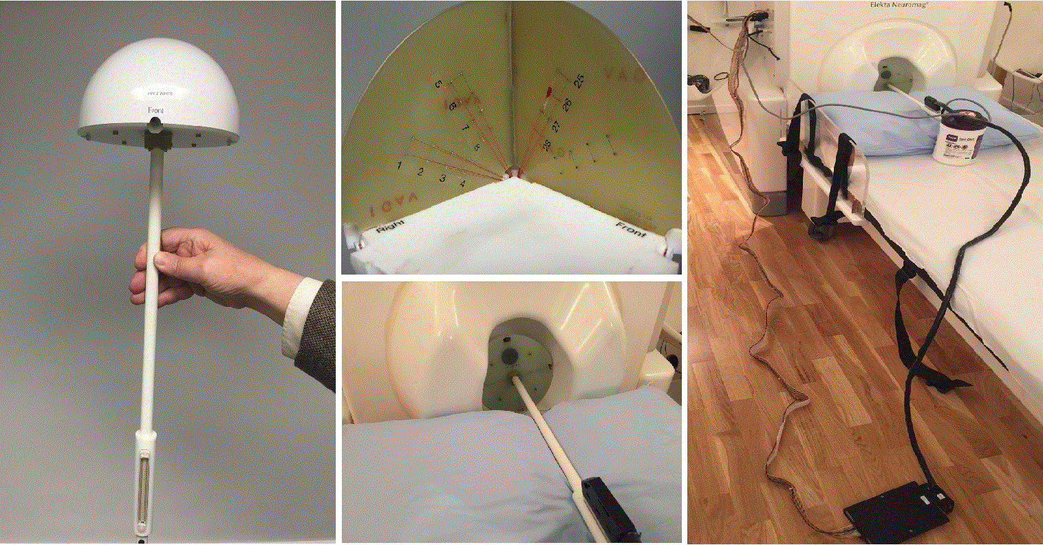
A current phantom is provided with the Elekta Neuromag for checking the system performance. It contains 32 artificial dipoles and four fixed head-position indicator coils. The phantom is based on the mathematical fact that an equilateral triangular line current produces equivalent magnetic field distribution to that of a tangential current dipole in a spherical conductor, provided that the vertex of the triangle and the origin of the conducting sphere coincide. For a detailed description of how the phantom works, see here.
The phantom dipoles are energized using an internal signal generator which also feeds the HPI coils. An external multiplexer box is used to connect the signal to the individual dipoles. Only one dipole can be activated at a time. The location of the dipole is recorded relative to the center of the sphere (0,0,0)m, where X is positive toward the nasion, Y is positive toward the left ear and Z is positive toward the top of the head (see the CoordinateSystems tutorial for more details).
Use of the phantom is shown below. Note that the uncovered version is the phantom that came with the Neuromag-122, which explicitly shows the wiring. The covered version uses the same principle but somewhat different dipole locations. Further details are available in Section 7.2 of the User's Manual.
References
- R.J. Ilmoniemi, M.S. Hämäläinen, and J. Knuutila, The Forward and Inverse Problems in the Spherical Model. In: Biomagnetism: Applications and Theory, eds. H. Weinberg, G. Stroink, T. Katil, Pergamon Press, 1985.
- Elekta Neuromag System Hardware User's Manual, Revision G, September 2005.
Description of the experiment
Files distributed as part of the phantom Elekta tutorial:
kojak_all_2000nAm_pp_no_chpi_no_ms_raw.fif
Source = 2000 nAm. This corresponds to an unrealistically strong 1,000 nA-m (2,000 nA-m peak to peak) dipole that gives the highest SNR visualization of the experimental source.kojak_all_200nAm_pp_no_chpi_no_ms_raw.fif
Source = 200 nAm. This is a weaker dipole, closer to the range of amplitudes we can expect from inter-ictal spikes due to epilepsy, visible in raw data.kojak_all_20nAm_pp_no_chpi_no_ms_raw.fif
Source = 20 nAm. This represents some of the weakest sources we expect in evoked studies which require averaging to detect and estimate (i.e. generally cannot be seen in single trials).- All recordings were performed by John Mosher in the MEG lab at the Cleveland Clinic with an Elekta phantom.
Download and installation
Requirements: You have followed the introduction tutorials and Brainstorm is installed.
Go to the Download page and download the file: sample_phantom_elekta.zip
- Unzip it in a folder that is not in any of the Brainstorm folders (program folder or database folder)
- Start Brainstorm (Matlab scripts or stand-alone version)
Select the menu File > Create new protocol. Name it TutorialPhantomElekta and select:
No, use individual anatomy,
No, use one channel file per acquisition run (MEG).
Generate anatomy
In the Matlab command window: type "generate_phantom_elekta".
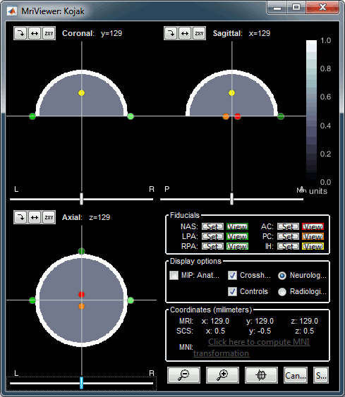
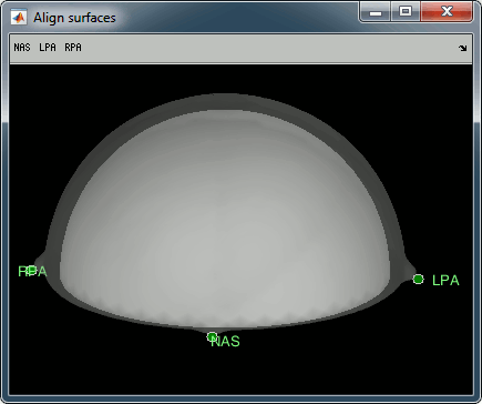
This creates a new subject Kojak (so named after the 70's TV show) and generates the "anatomy" for this device: one volume and a few surfaces representing the geometry of the phantom.
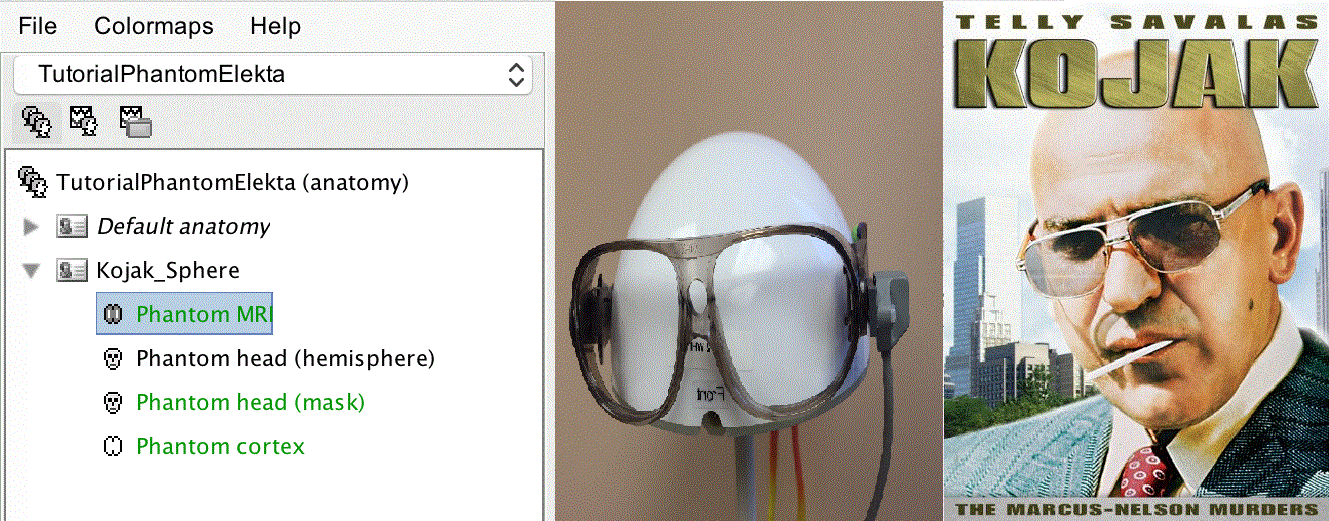
You can display the MRI and surfaces as presented in the introduction tutorials.
Access the recordings
We can now review one of the raw kojak data sets. These have been generated by sequentially activating each of the 32 phantom dipoles in a single raw file.
Switch to the functional data view by clicking the second button under the protocol name.
Right-click on the subject folder > Review raw file.
Select the 200nA source.
Click Event channel, select STI201, and hit OK.
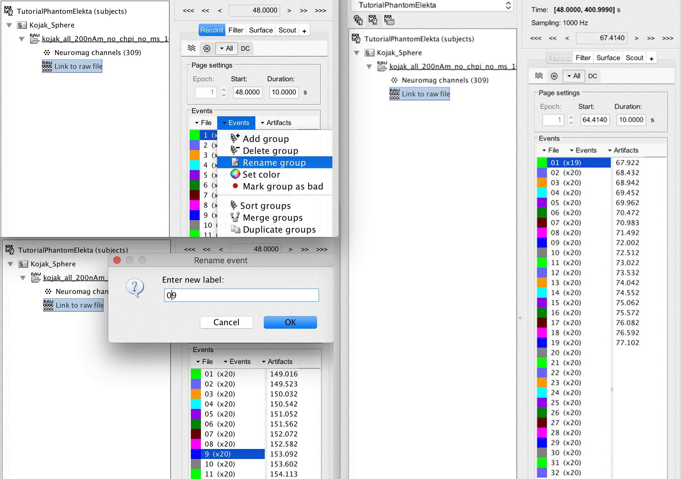
Close the figure and double click the link to raw file to open a list of the events. At this point, you may wish to rename your groups so that the ordering remains convenient. To do this, click group 1, click Events > Rename group, and rename it to 01. Repeat this for 2 - 9.
This step, and others like it, can also be performed by importing the data into MATLAB, running the following code below, and then exporting the data back into Brainstorm:
% to change the trigger numbers to appear sequentially
for i = 1:32,
    STR = str2num(link_filename.F.events(i).label);
    link_filename.F.events(i).label = sprintf('%02.0f',STR);
end
Some other triggers are generated by the neuromag system which are unnecessary so we will delete them:
Trim away the singleton events by clicking on 256 (x1), shift clicking on 7936 (x1) and pressing the delete key.
There is also a switching transient in the phantom generator which should be removed:
Remove the first event from dipole 01 by clicking on it, clicking on the first time instant, and pressing the delete key.
Events should now appear as per the image below on the right:
Note: Make sure to save the modifications that you make before proceeding. If you hit the grey X to close all figures and clear memory, you will be prompted to save modifications, and you should click Yes.
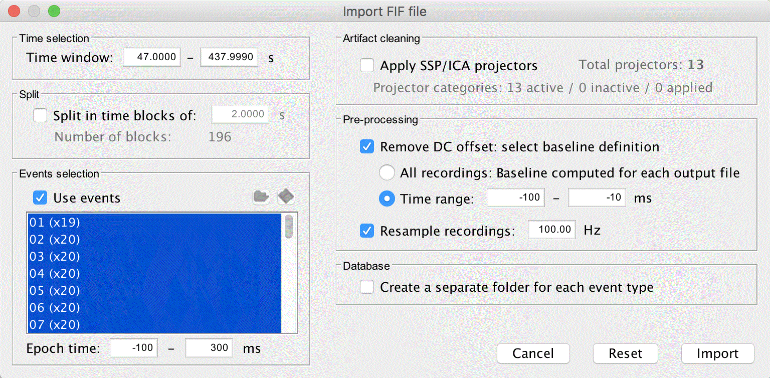
Importing the dipole events
Right click on Link to raw file and click Import in database
Uncheck Apply SSP/ICA projectors (we will use noise covariance to stabilize the data)
Check Remove DC offset, set the time range from -100 to -10ms
Resample the recordings to 100Hz (change from 1000Hz)
Do not create separate folders
Click Import
Noise covariance
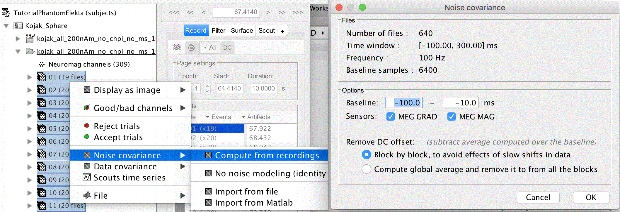
With the epochs loaded, we can now calculate the noise covariance from the prestims. To do this, select all 32 dipoles (click the first then shift click the last), then right click, Noise covariance > Compute from recordings. Uncheck MEG MAG and hit OK.
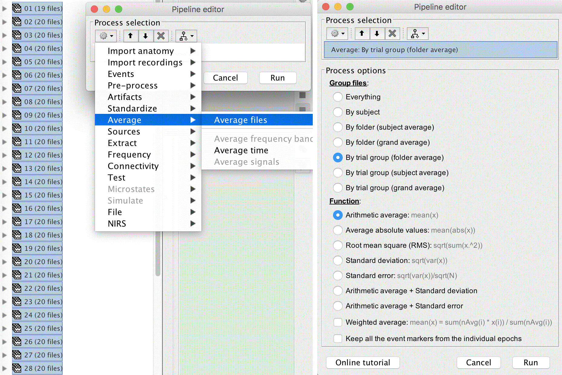
Average all of the epochs by selecting all 32 again, dragging them to the process box, clicking RUN. Next click the cog, and select Average > Average files. Group the files By trial group (folder average), and select Arithmetic average: mean(x), and click "Run".
Head modelling
To compute the head model, right click on the kojak_all_200nA file and select Compute head model.
Source space: select MRI volume
Forward modeling methods: Single sphere
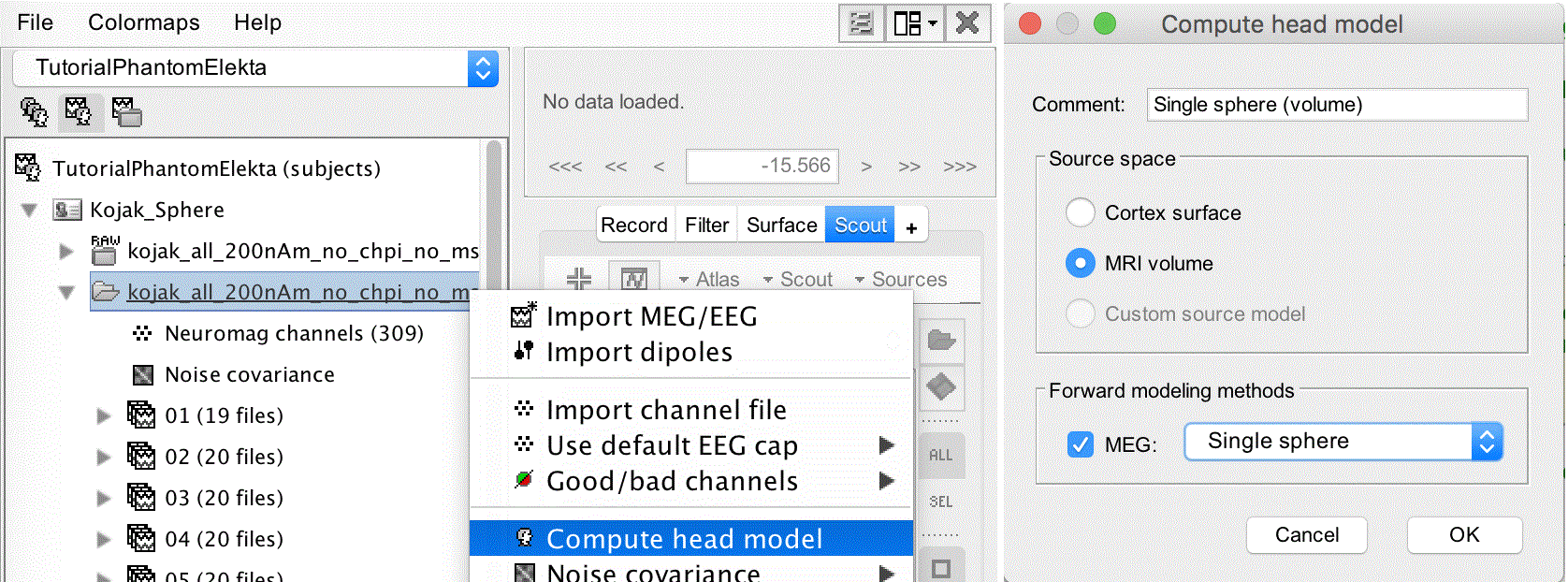
A figure opens showing a sphere fit to the phantom, however we can see that the location is a little off. In this case we alread know where the center of the sphere should be, so we adjust it manually:
Click the Edit sphere properties button in the top toolbar.
Change the center location to [ 0 0 0 ] and hit OK.
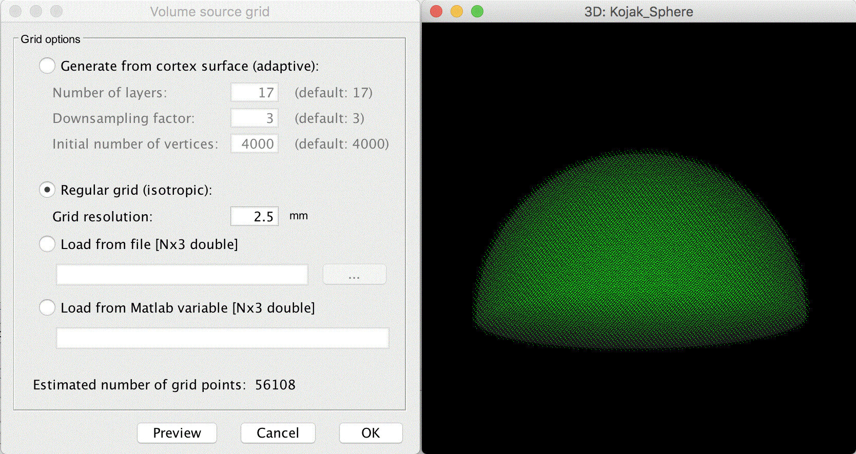
The center of the sphere shifts to the correct position. Click the OK button next to the edit sphere properties button to perform the MRI/surface interpolation. A window appears allowing adjustment of the volume source grid.
Select Regular grid (isotropic) with Grid resolution 2.5mm
This results in an around 56K grid point, which is sufficient.
Dipole source estimation
Right click the Single sphere (volume) and select Compute sources [2016]
Method: Dipole modeling
Source model: Dipole orientations Unconstrained
For the sensor selection you can choose to use either the gradiometers or the magnetometers, in this case we select both.
Click Show details if the noise covariance regularization is hidden.
Select Regularize noise covariance: 0.1
Ignore the other settings, and click OK
Dipole scanning
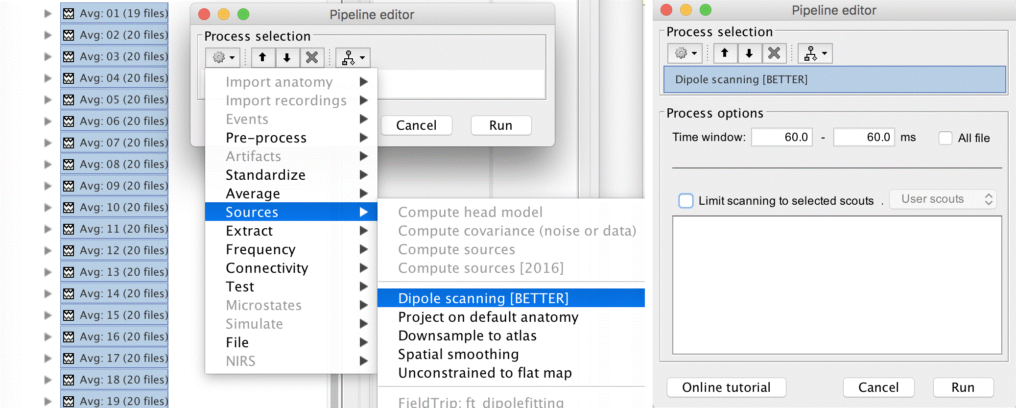
Select the set of 32 averages and drop them into the process box again. Switch to process sources and click the cog in the pipeline editor. Select Sources > Dipole Scanning [BETTER]. Set the process options to look at 60ms only by changing the Time window to 60ms - 60ms, and clicking Run.
Next we should average all the dipole fits together. To do this, we can expand the tree of average files and select Avg: 01 (19 files) | dipole scan through Avg: 32 (20 files) | dipole scan, then right click and select Merge dipoles. Alternatively, we can set Matlab to the study directory and use
FILES = dir('dipoles_fit*');
new = dipoles_merge({FILES.name});
As an optional step, we can sign flip the dipoles in Matlab so that they are all pointing up for convenience. To do this, right click on Merge: 32 files and export to Matlab as the variable merge_dips. Then in Matlab use the following code:
for i = 1:32,
    merge_dips.Dipole(i).Amplitude = merge_dips.Dipole(i).Amplitude*...
    sign(merge_dips.Dipole(i).Amplitude(3));
end
merge_dips.Comment = [merge_dips.Comment ' | flipped'];
You can then right click on the channel file and click File > Import from Matlab, and bring merge_dips back into Brainstorm. With the comment added to the file, it should appear next to the previous merged dipoles, as Merge: 32 files | flipped.
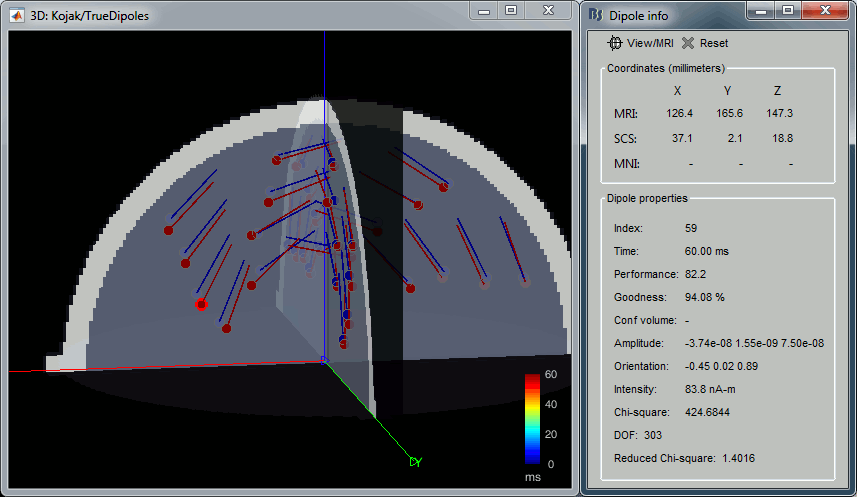
Right click on the flippled dipole merge and click Diplay on MRI (3D), which brings up a figure showing the dipole locations. To compare these to the true locations in Matlab, you can run the following code:
[true_dipole_mat,true_loc,true_orient] = generate_phantom_neuromag_dips;

hold on
hq = quiver3(true_loc(1,:),true_loc(2,:),true_loc(3,:),...
     true_orient(1,:),true_orient(2,:),true_orient(3,:));
hold off
set(hq,'color','r'),shg
The true dipole locations are now shown in red along with the estimated locations in blue:
Results
  Dipole      Loc (mm)      Amp (nA-m)  Gof     Perf       Chi2     RChi2
--------------------------------------------------------------------------
  01 - [ -0.4 -60.4  21.3]    75.1    98.8%    208.7    513 (201)   2.55
  02 - [  2.1 -47.9  21.3]    83.3    97.9%    117.4    295 (201)   1.47
  03 - [ -0.4 -35.4  23.8]    79.8    94.1%     64.5    263 (201)   1.31
  04 - [ -0.4 -25.4  21.3]    74.6    83.9%     36.2    251 (201)   1.25
  05 - [  2.1 -35.4  48.8]    92.7    98.1%    154.3    466 (201)   2.32
  06 - [  2.1 -25.4  43.8]    91.4    96.8%     87.9    256 (201)   1.27
  07 - [  2.1 -15.4  38.8]    90.7    91.9%     53.2    251 (201)   1.25
  08 - [  2.1  -5.4  33.8]    77.7    80.9%     30.6    222 (201)   1.10
  09 - [-60.4   2.1  21.3]    77.3    98.6%    204.2    584 (201)   2.91
  10 - [-47.9   2.1  23.8]    82.2    98.0%    120.0    290 (201)   1.44
  11 - [-35.4  -0.4  23.8]    83.9    94.8%     69.1    262 (201)   1.30
  12 - [-25.4   2.1  21.3]    80.4    88.9%     42.3    224 (201)   1.12
  13 - [-35.4   2.1  51.3]    84.4    98.4%    178.3    507 (201)   2.52
  14 - [-27.9   2.1  43.8]    86.0    96.9%    101.7    326 (201)   1.62
  15 - [-15.4   2.1  38.8]    89.3    93.5%     60.9    258 (201)   1.28
  16 - [ -7.9   2.1  31.3]    80.4    83.1%     35.2    251 (201)   1.25
  17 - [ -0.4  47.1  41.3]    85.8    98.7%    176.4    423 (201)   2.10
  18 - [ -0.4  44.6  31.3]    77.1    98.0%    106.0    229 (201)   1.14
  19 - [ -0.4  42.1  18.8]    72.7    94.5%     68.7    273 (201)   1.36
  20 - [ -0.4  34.6   8.8]    74.4    88.8%     42.3    224 (201)   1.12
  21 - [ -0.4  14.6  61.3]    79.5    98.3%    131.7    306 (201)   1.52
  22 - [  2.1  17.1  48.8]    87.9    96.1%     82.1    274 (201)   1.36
  23 - [  2.1  22.1  36.3]    86.4    92.5%     55.9    253 (201)   1.26
  24 - [  2.1  19.6  23.8]    91.6    84.0%     36.7    258 (201)   1.28
  25 - [ 47.1   2.1  41.3]    88.1    97.1%     94.2    264 (201)   1.31
  26 - [ 42.1  -0.4  31.3]    83.7    93.9%     61.7    247 (201)   1.23
  27 - [ 37.1  -0.4  18.8]    87.5    88.9%     45.6    260 (201)   1.29
  28 - [ 29.6   2.1  11.3]    85.3    87.7%     32.7    151 (201)   0.75
  29 - [ 14.6   2.1  58.8]    92.1    97.6%    129.1    402 (201)   2.00
  30 - [ 17.1   2.1  48.8]    86.8    95.8%     76.7    257 (201)   1.28
  31 - [ 19.6   2.1  38.8]    80.1    91.3%     48.3    223 (201)   1.11
  32 - [ 22.1   2.1  23.8]    87.2    84.6%     34.3    213 (201)   1.06


 Location errors from true

 Dipole      Loc (mm)            True (mm)         Diff [x y z]     Norm (mm)
------------------------------------------------------------------------------
  01 - [ -0.4 -60.4  21.3] [  0.0 -59.7  22.9] [ -0.4  -0.7  -1.6]   (  1.8)
  02 - [  2.1 -47.9  21.3] [  0.0 -48.6  23.5] [  2.1   0.7  -2.2]   (  3.2)
  03 - [ -0.4 -35.4  23.8] [  0.0 -35.8  25.5] [ -0.4   0.4  -1.7]   (  1.8)
  04 - [ -0.4 -25.4  21.3] [  0.0 -24.8  23.1] [ -0.4  -0.6  -1.8]   (  2.0)
  05 - [  2.1 -35.4  48.8] [  0.0 -37.2  52.0] [  2.1   1.8  -3.2]   (  4.3)
  06 - [  2.1 -25.4  43.8] [  0.0 -27.5  46.4] [  2.1   2.1  -2.6]   (  4.0)
  07 - [  2.1 -15.4  38.8] [  0.0 -15.8  41.0] [  2.1   0.4  -2.2]   (  3.1)
  08 - [  2.1  -5.4  33.8] [  0.0  -7.9  33.0] [  2.1   2.5   0.8]   (  3.4)
  09 - [-60.4   2.1  21.3] [-59.7  -0.0  22.9] [ -0.7   2.1  -1.6]   (  2.7)
  10 - [-47.9   2.1  23.8] [-48.6  -0.0  23.5] [  0.7   2.1   0.3]   (  2.2)
  11 - [-35.4  -0.4  23.8] [-35.8  -0.0  25.5] [  0.4  -0.4  -1.7]   (  1.8)
  12 - [-25.4   2.1  21.3] [-24.8  -0.0  23.1] [ -0.6   2.1  -1.8]   (  2.8)
  13 - [-35.4   2.1  51.3] [-37.2  -0.0  52.0] [  1.8   2.1  -0.7]   (  2.9)
  14 - [-27.9   2.1  43.8] [-27.5  -0.0  46.4] [ -0.4   2.1  -2.6]   (  3.4)
  15 - [-15.4   2.1  38.8] [-15.8  -0.0  41.0] [  0.4   2.1  -2.2]   (  3.1)
  16 - [ -7.9   2.1  31.3] [ -7.9  -0.0  33.0] [  0.0   2.1  -1.7]   (  2.7)
  17 - [ -0.4  47.1  41.3] [  0.0  46.1  44.4] [ -0.4   1.0  -3.1]   (  3.3)
  18 - [ -0.4  44.6  31.3] [  0.0  41.9  34.0] [ -0.4   2.7  -2.7]   (  3.8)
  19 - [ -0.4  42.1  18.8] [  0.0  38.3  21.6] [ -0.4   3.8  -2.8]   (  4.7)
  20 - [ -0.4  34.6   8.8] [  0.0  31.5  12.7] [ -0.4   3.1  -3.9]   (  5.0)
  21 - [ -0.4  14.6  61.3] [  0.0  13.9  62.4] [ -0.4   0.7  -1.1]   (  1.4)
  22 - [  2.1  17.1  48.8] [  0.0  16.2  51.5] [  2.1   0.9  -2.7]   (  3.6)
  23 - [  2.1  22.1  36.3] [  0.0  20.0  39.1] [  2.1   2.1  -2.8]   (  4.1)
  24 - [  2.1  19.6  23.8] [  0.0  19.3  27.9] [  2.1   0.3  -4.1]   (  4.7)
  25 - [ 47.1   2.1  41.3] [ 46.1  -0.0  44.4] [  1.0   2.1  -3.1]   (  3.9)
  26 - [ 42.1  -0.4  31.3] [ 41.9  -0.0  34.0] [  0.2  -0.4  -2.7]   (  2.8)
  27 - [ 37.1  -0.4  18.8] [ 38.3  -0.0  21.6] [ -1.2  -0.4  -2.8]   (  3.1)
  28 - [ 29.6   2.1  11.3] [ 31.5  -0.0  12.7] [ -1.9   2.1  -1.4]   (  3.1)
  29 - [ 14.6   2.1  58.8] [ 13.9  -0.0  62.4] [  0.7   2.1  -3.6]   (  4.2)
  30 - [ 17.1   2.1  48.8] [ 16.2  -0.0  51.5] [  0.9   2.1  -2.7]   (  3.6)
  31 - [ 19.6   2.1  38.8] [ 20.0  -0.0  39.1] [ -0.4   2.1  -0.3]   (  2.1)
  32 - [ 22.1   2.1  23.8] [ 19.3  -0.0  27.9] [  2.8   2.1  -4.1]   (  5.4)


 Orientation errors from true

 Dipole  Amp (nA-m)      [X Y Z]              TRUE [X Y Z]     Degrees
------------------------------------------------------------------------
  01 -    ( 75.1)  [-0.01  0.31  0.95] vs [ 0.00  0.36  0.93] (  3.0 )
  02 -    ( 83.3)  [-0.02  0.38  0.93] vs [ 0.00  0.44  0.90] (  3.7 )
  03 -    ( 79.8)  [-0.09  0.52  0.85] vs [ 0.00  0.58  0.81] (  6.5 )
  04 -    ( 74.6)  [-0.10  0.60  0.79] vs [ 0.00  0.68  0.73] (  8.2 )
  05 -    ( 92.7)  [-0.03  0.79  0.61] vs [ 0.00  0.81  0.58] (  2.7 )
  06 -    ( 91.4)  [-0.02  0.85  0.53] vs [ 0.00  0.86  0.51] (  2.0 )
  07 -    ( 90.7)  [-0.02  0.91  0.41] vs [ 0.00  0.93  0.36] (  3.2 )
  08 -    ( 77.7)  [ 0.10  0.98  0.19] vs [ 0.00  0.97  0.23] (  6.0 )
  09 -    ( 77.3)  [ 0.32  0.03  0.95] vs [ 0.36  0.00  0.93] (  3.0 )
  10 -    ( 82.2)  [ 0.43  0.08  0.90] vs [ 0.44  0.00  0.90] (  4.7 )
  11 -    ( 83.9)  [ 0.53  0.10  0.84] vs [ 0.58  0.00  0.81] (  6.7 )
  12 -    ( 80.4)  [ 0.61  0.20  0.76] vs [ 0.68  0.00  0.73] ( 12.1 )
  13 -    ( 84.4)  [ 0.82  0.02  0.58] vs [ 0.81  0.00  0.58] (  1.5 )
  14 -    ( 86.0)  [ 0.84  0.02  0.55] vs [ 0.86  0.00  0.51] (  2.8 )
  15 -    ( 89.3)  [ 0.92  0.10  0.37] vs [ 0.93  0.00  0.36] (  6.0 )
  16 -    ( 80.4)  [ 0.96  0.13  0.25] vs [ 0.97  0.00  0.23] (  7.3 )
  17 -    ( 85.8)  [ 0.00 -0.66  0.75] vs [ 0.00 -0.69  0.72] (  2.7 )
  18 -    ( 77.1)  [-0.05 -0.57  0.82] vs [ 0.00 -0.63  0.78] (  5.2 )
  19 -    ( 72.7)  [-0.13 -0.39  0.91] vs [ 0.00 -0.49  0.87] (  9.5 )
  20 -    ( 74.4)  [-0.15 -0.22  0.96] vs [ 0.00 -0.37  0.93] ( 12.3 )
  21 -    ( 79.5)  [-0.10 -0.97  0.22] vs [ 0.00 -0.98  0.22] (  5.6 )
  22 -    ( 87.9)  [-0.08 -0.95  0.32] vs [ 0.00 -0.95  0.30] (  4.5 )
  23 -    ( 86.4)  [-0.11 -0.85  0.51] vs [ 0.00 -0.89  0.46] (  7.3 )
  24 -    ( 91.6)  [-0.18 -0.75  0.63] vs [ 0.00 -0.82  0.57] ( 11.8 )
  25 -    ( 88.1)  [-0.65  0.03  0.76] vs [-0.69  0.00  0.72] (  3.8 )
  26 -    ( 83.7)  [-0.58 -0.01  0.81] vs [-0.63  0.00  0.78] (  3.6 )
  27 -    ( 87.5)  [-0.43 -0.03  0.90] vs [-0.49  0.00  0.87] (  4.3 )
  28 -    ( 85.3)  [-0.32 -0.04  0.95] vs [-0.37  0.00  0.93] (  4.1 )
  29 -    ( 92.1)  [-0.97 -0.02  0.25] vs [-0.98  0.00  0.22] (  2.0 )
  30 -    ( 86.8)  [-0.94 -0.02  0.34] vs [-0.95  0.00  0.30] (  2.5 )
  31 -    ( 80.1)  [-0.89 -0.00  0.46] vs [-0.89  0.00  0.46] (  0.5 )
  32 -    ( 87.2)  [-0.71 -0.00  0.70] vs [-0.82  0.00  0.57] (  9.7 )
Scripting
Generate Matlab script
Available in the Brainstorm distribution: brainstorm3/toolbox/script/tutorial_phantom_elekta.m

