|
⇤ ← Revision 1 as of 2017-12-01 11:02:37
Size: 29649
Comment:
|
Size: 29619
Comment:
|
| Deletions are marked like this. | Additions are marked like this. |
| Line 1: | Line 1: |
| = MEG visual tutorial: Group analysis = | = MEG visual tutorial: Single subject = |
| Line 4: | Line 4: |
| The aim of this tutorial is to reproduce in the Brainstorm environment the analysis described in the SPM tutorial "[[ftp://ftp.mrc-cbu.cam.ac.uk/personal/rik.henson/wakemandg_hensonrn/Publications/SPM12_manual_chapter.pdf|Multimodal, Multisubject data fusion]]". The data processed here consists in simultaneous MEG/EEG recordings of 19 subjects performing a simple visual task on a large number of famous, unfamiliar and scrambled faces. This tutorial follows another page that explains how to process [[Tutorials/VisualSingle|one single subject]] in details. | The aim of this tutorial is to reproduce in the Brainstorm environment the analysis described in the SPM tutorial "[[ftp://ftp.mrc-cbu.cam.ac.uk/personal/rik.henson/wakemandg_hensonrn/Publications/SPM12_manual_chapter.pdf|Multimodal, Multisubject data fusion]]". The data processed here consists of simultaneous MEG/EEG recordings from 19 participants performing a simple visual recognition task from presentations of famous, unfamiliar and scrambled faces. The analysis is split in two tutorial pages: the present tutorial describes the detailed analysis of one single subject; the second tutorial describes batch processing and [[Tutorials/VisualGroup|group analysis of all 19 participants]]. Note that the operations used here are not detailed, the goal of this tutorial is not to introduce Brainstorm to new users. For in-depth explanations of the interface and theoretical foundations, please refer to the [[http://neuroimage.usc.edu/brainstorm/Tutorials#Get_started|introduction tutorials]]. |
| Line 9: | Line 13: |
| This dataset was obtained from the OpenfMRI project (http://www.openfmri.org), accession #ds117. It is made available under the Creative Commons Attribution 4.0 International Public License. Please cite the following reference if you use these data: <<BR>>Wakeman DG, Henson RN, [[http://www.nature.com/articles/sdata20151|A multi-subject, multi-modal human neuroimaging dataset]], Scientific Data (2015) Any questions, please contact: rik.henson@mrc-cbu.cam.ac.uk |
This dataset was obtained from the OpenfMRI project (http://www.openfmri.org), accession #ds117. It is made available under the Creative Commons Attribution 4.0 International Public License. Please cite the following reference if you use these data: <<BR>>Wakeman DG, Henson RN, [[http://www.nature.com/articles/sdata20151|A multi-subject, multi-modal human neuroimaging dataset]], Scientific Data (2015) Any questions regarding the data, please contact: rik.henson@mrc-cbu.cam.ac.uk == Presentation of the experiment == ==== Experiment ==== * 19 subjects (three were excluded from the group analysis for [[http://neuroimage.usc.edu/brainstorm/Tutorials/VisualSingle#Bad_subjects|various reasons]]) * 6 acquisition runs (aka sessions) of approximately 10mins for each subject * Presentation of series of images: familiar faces, unfamiliar faces, phase-scrambled faces * Participants had to judge the left-right symmetry of each stimulus * Total of nearly 300 trials for each of the 3 conditions ==== MEG acquisition ==== * Acquisition at 1100Hz with an Elekta-Neuromag VectorView system (simultaneous MEG+EEG). * Recorded channels (404): * 102 magnetometers * 204 planar gradiometers * 70 EEG electrodes recorded with a nose reference. * MEG data have been "cleaned" using Signal-Space Separation as implemented in MaxFilter 2.2. * A Polhemus device was used to digitize three fiducial points and a large number of other points across the scalp, which can be used to coregister the M/EEG data with the structural MRI image. * Stimulation triggers: The triggers related with the visual presentation are saved in the STI101 channel, with the following event codes (bit 3 = face, bit 4 = unfamiliar, bit 5 = scrambled): * Famous faces: 5 (00101), 6 (00110), 7 (00111) * Unfamiliar faces: 13 (01101), 14 (01110), 15 (01111) * Scrambled images: 17 (10001), 18 (10010), 19 (10011) * Delays between the trigger in STI101 and the actual presentation of stimulus: '''34.5ms''' * The data distribution includes MEG noise recordings acquired around the dates of the experiment, processed with MaxFilter 2.2 in the same way as the experimental data. ==== Subject anatomy ==== * MRI data acquired on a 3T Siemens TIM Trio: 1x1x1mm T1-weighted structural MRI. * The face was removed from the strucural images for anonymization purposes. * Processed with FreeSurfer 5.3. |
| Line 14: | Line 46: |
| First, make sure you have enough space on your hard drive, at least '''40Gb''': * The Brainstorm database with all the data imported, downloaded from this website: '''20Gb''' * The same database after this tutorial: '''40Gb''' You can follow this tutorial after processing the recordings for the 16 good subjects (6 runs per subject) as illustrated in the [[Tutorials/VisualSingle|single subject tutorial]]. Otherwise, we provide a Brainstorm protocol that includes all the imported data, downsampled at 275Hz: * Go to the [[http://neuroimage.usc.edu/bst/download.php|Download]] page, download the file '''TutorialGroup.zip''' (20Gb). * Unzip this file in your Brainstorm database folder (brainstorm_db). * In Brainstorm, menu File > Load protocol > Load from folder > Select '''brainstorm_db/TutorialGroup''' The database you need in order to follow this tutorial should contain the following: * The individual anatomy imported from FreeSurfer or BrainSuite for each subject (16 subjects). * The sensor level averages (MEG+EEG) for each run (downsampled to 275Hz or not). * The forward model, noise covariance and inverse models for each subject and each run. <<BR>><<BR>> {{attachment:db_tutorialgroup.gif||width="422",height="346"}} * This protocol TutorialGroup is produced from the single subject protocol TutorialVisual with the script: '''brainstorm3/toolbox/script/tutorial_visual_copy.m''' <<BR>><<BR>><<HTML(<div style="border:1px solid black; background-color:#EEEEFF; width:680px; height:250px; overflow:scroll; padding:10px; font-family: Consolas,Menlo,Monaco,Lucida Console,Liberation Mono,DejaVu Sans Mono,Bitstream Vera Sans Mono,Courier New,monospace,sans-serif; font-size: 13px; white-space: pre;">)>><<EmbedContent("http://neuroimage.usc.edu/bst/viewcode.php?f=tutorial_visual_copy.m")>><<HTML(</div >)>> * If you are not using the package TutorialGroup.zip, make sure you exclude the bad subjects from the analysis: sub001, sub005, sub016. You would also need to add some selection processes to select only the averages (and not the continuous recordings or the individual trials). == Overview of the analysis == === Coregistration of the acquisition runs === For each subject, all the runs have been registered to a common head position with MaxFilter. To verify this, select all the channel files within one subject, right-click > Display sensors > MEG (all). The surfaces representing the MEG helmet are perfectly overlapping for all the runs. When the runs are not aligned, it looks like [[http://neuroimage.usc.edu/brainstorm/Tutorials/ChannelFile#Multiple_runs_and_head_positions|this]]. . {{attachment:run_coreg.gif||width="486",height="163"}} This means we can safely average or compare the MEG sensor values across runs within one subject. However, it is not reliable to average MEG recordings across subjects, because of the [[http://neuroimage.usc.edu/brainstorm/Tutorials/Workflows#MEG_recordings|anatomical differences between subjects]]. This doesn't mean we can estimate the sources only once per subject. We have computed different SSP projectors and selected different bad channels for each acquisition run. To be able to use this information efficiently we should estimate the sources for each run separately, then average the sources across runs. The forward model is the same for all the runs within one subject, therefore it can be computed for the first run and copied to all the other runs. === Objectives === The objectives for this tutorial are to reproduce the analysis presented in the following documents: * Wakeman DG, Henson RN, [[http://www.nature.com/articles/sdata20151|A multi-subject, multi-modal human neuroimaging dataset]]<<BR>>Scientific Data (2015) * Wakeman DG, Henson RN, [[ftp://ftp.mrc-cbu.cam.ac.uk/personal/rik.henson/wakemandg_hensonrn/Publications/WakemanHenson_biomag2010_poster.pdf|Functional and structural connrctivity in face processing: MEG, EEG, fMRI, MRI and DWI data]], Biomag 2016 * SPM12 manual, chapter 41: [[ftp://ftp.mrc-cbu.cam.ac.uk/personal/rik.henson/wakemandg_hensonrn/Publications/SPM12_manual_chapter.pdf|Multimodal, Multisubject data fusion]] Summary of the results we will compute in this tutorial: * Subject and grand averages for each condition (Famous, Unfamiliar, Scrambled). * Normalization of these averages (Z-score for the sources, or ERS/D for the time-frequency maps). * Projection of the sources results on a template and spatial smoothing of the source maps. * Contrast between faces (famous+unfamiliar) and non-faces (scrambled): difference of averages and significance test. * Contrast between famous faces and unfamiliar faces: difference of averages and significance test. * Sensors of interest: EEG070 (or EEG060 or EEG065 if EEG070 is marked as bad) Expected effects: * OFA: Bilateral occipital face area * FFA: Bilateral fusiform face area * STS: Right superior temporal sulcus * Around 170ms (N170): Difference between Faces and Scrambled. * After 250ms: Difference between Famous and Unfamiliar. The methodology that we will follow for computing the averages and the other statistics is described in the tutorial "[[Tutorials/Workflows|Workflows]]". == Subject averages: Famous, Unfamiliar, Scrambled == We will start by computing the subject-level averages for all the data types we have: sensor-level recordings, source maps and time-frequency results. We will use a weighted average to group the results we have for each run (weighted by the number of good trials). We want to compute the averages for each experimental condition separately (famous, unfamiliar, scrambled). Since the files are already selected in the interface, we will also compute a grand average across subject. In this context, we will consider that each subject has the same weight in the grand average (option "weighted" not selected). Note that it is not accurate to average MEG recordings across subjects, but we can do it just to get a general idea of the group effects ([[http://neuroimage.usc.edu/brainstorm/Tutorials/Workflows#MEG_recordings|more information]]). === MEG/EEG === * Drag and drop all the subjects in Process1. Select button '''[Process recordings]'''. * Select process '''Average > Average files''': '''By trial group (subject average)'''<<BR>>Arithmetic average, Weighted * Add process '''Average > Average files''': '''By trial group (grand average)'''<<BR>>Arithmetic average, __Not__ weighted <<BR>><<BR>> {{attachment:average_process_data.gif||width="492",height="500"}} * In output, you get three grand averages in the "Group analysis/Inter-subject" folder (top), and three subject averages per subject in the "intra-subject" folders (bottom). {{attachment:average_files_data.gif||width="653",height="273"}} === Sources === * Keep all the subjects selected in Process1. Select button '''[Process sources]'''. * If you run the averaging process directly with this file selection, it would average together the MEG and the EEG sources (36 files selected per subject instead of 18). To average separately the two modalities, we can use the '''Filter''' box at the bottom-right corner of the Brainstorm window. Enter "EEG" and it would select only the files with a comment including the tag "EEG". * Select process '''Average > Average files''': '''By trial group (subject average)'''<<BR>>EEG source files only, Arithmetic average, Weighted * Add process '''File > Add tag''': '''EEG'''.<<BR>><<BR>> {{attachment:average_process_sources.gif||width="603",height="504"}} * Repeat the same steps with the '''MEG''' source files (select all subjects, filter, average, tag). * This time, we cannot compute a grand average directly because the source spaces used to estimate the brain activity do not match between subjects. We have to go through an additional step of projection on a template anatomy. We will also wait to have normalized the source maps before displaying them.<<BR>><<BR>> {{attachment:average_files_sources.gif||width="243",height="208"}} === Time-frequency === * Keep all the subjects selected in Process1. Select button '''[Process time-freq]'''.<<BR>>Make sure you reset the Filter search box at the bottom-right of the Brainstorm window. * Run process '''Average > Average files''': '''By trial group (subject average)'''<<BR>>Arithmetic average, Weighted, Match signals<<BR>><<BR>> {{attachment:average_process_tf.gif||width="415",height="498"}} * Like for the sources, we will first normalize the time-frequency maps with respect with a baseline before computing grand averages. Like the sensor data: it is valid to average EEG recordings across subjects, but it is not accurate to average MEG sensors across subjects. * We can average the time-frequency files across runs (it is as valid as averaging the MEG or EEG signals), wut we need to select this option "match signals between files using their names" to account for the variable number of bad channels we may have across runs or subjects. <<BR>><<BR>> {{attachment:average_files_tf.gif||width="633",height="250"}} == Subject averages: Faces == One of the contrast we want to study is faces (Famous and Unfamiliar) vs non-faces (Scrambled). We need to re-average the Famous and Unfamiliar averages together. === MEG/EEG === * In Process2: FilesA = all the Famous subject averages, FilesB = all the Unfamiliar subject averages. The subjects must be in the same order in the two lists because the process will process the files by pairs of files (A,B). * Select process '''Other > Average A&B''': Weighted.<<BR>>Add process '''File > Set comment''': Comment = "WAvg: Avg: Faces"<<BR>>Add process '''Average > Average files''': '''By trial group (subject average)''': __Not__ weighted<<BR>><<BR>> {{attachment:average_faces_data.gif||width="669",height="531"}} * Selecting that many files from the database explorer can be long when done manually, but can be very efficient from a script. Check out the script equivalent at the end of this page. * It creates one new average for each pair (A,B) and computes the grand average for condition Faces. <<BR>><<BR>> {{attachment:average_faces_data2.gif||width="299",height="234"}} === Sources === * In Process2: FilesA = all the '''Famous '''subject averages (EEG only) [Process sources] * In Process2: FilesB = all the '''Unfamiliar''' subject averages (EEG only) [Process sources] * Make sure the order of the files matches in the two lists. * Select process '''Other > Average A&B''': Weighted.<<BR>>Add process '''File > Set comment''': Comment = "WAvg: Avg: Faces | EEG"<<BR>><<BR>> {{attachment:average_faces_sources.gif||width="614",height="356"}} * Repeat the same steps for the '''MEG''' sources.<<BR>><<BR>> {{attachment:average_faces_sources2.gif||width="265",height="270"}} === Time-frequency === * In Process2: FilesA = all the '''Famous''' subject averages (EEG only) [Process timefreq] * In Process2: FilesB = all the '''Unfamiliar''' subject averages (EEG only) [Process timefreq] * Select process '''Other > Average A&B''': Weighted.<<BR>>Add process '''File > Set comment''': Comment = "WAvg: Avg: Faces"<<BR>><<BR>> {{attachment:average_faces_timefreq.gif||width="604",height="331"}} * In output: the average for the Face condition, for each subject. <<BR>><<BR>> {{attachment:average_faces_timefreq2.gif||width="284",height="76"}} == Subject averages: Within-subject differences == To detect correctly the differences between two conditions at the source level, we need to estimate the differences of the conditions for each subject, and then normalize the difference (see tutorial [[http://neuroimage.usc.edu/brainstorm/Tutorials/Workflows#Constrained_cortical_sources|Workflows]]). === Sources: Faces - Scrambled === * In Process2: FilesA = all the '''Faces''' subject averages (EEG only) [Process sources] * In Process2: FilesB = all the '''Scrambled''' subject averages (EEG only) [Process sources] * Select process '''Difference > Difference A-B''': Do __'''not'''__ use absolute values. * Add process '''File > Set comment''': Comment='''Faces - Scrambled | EEG''' <<BR>><<BR>> {{attachment:diffsubj_faces.gif||width="606",height="331"}} * Repeat the same steps for the '''MEG''' sources. === Sources: Famous - Unfamiliar === * In Process2: FilesA = all the '''Famous''' subject averages (EEG only) [Process sources] * In Process2: FilesB = all the '''Unfamiliar''' subject averages (EEG only) [Process sources] * Select process '''Difference > Difference A-B''': Do __'''not'''__ use absolute values. * Add process '''File > Set comment''': Comment='''Famous - Unfamiliar | EEG''' * Repeat the same steps for the '''MEG''' sources. <<BR>><<BR>> {{attachment:diffsubj_files.gif||width="284",height="240"}} == Subject averages: Filter and normalize == Before comparing the averages across subjects we are going to low-pass filter the signals below 32Hz (to smooth possible latency differences between subjects) and normalize the source and time-frequency values with respect with a baseline (see tutorial [[http://neuroimage.usc.edu/brainstorm/Tutorials/Workflows#Constrained_cortical_sources|Workflows]]). === MEG/EEG === * In Process1, select all the '''Intra-subject''' folders from all the subjects, select '''[Process recordings]'''. For a faster selection, you can use the view "Functional data (sorted by conditions)". * Select process '''Pre-process > Band-pass filter''': 0Hz-32Hz, MEG,EEG, 60dB, No mirror, Overwrite. * Add process '''Extract > Extract time''': Time window='''[-200,900]ms''' <<BR>><<BR>> {{attachment:filter_data_process.gif||width="622",height="320"}} * Two tags are added at the end of the comments of the averaged recordings. The selection of a smaller time window gets rid of most of the possible edge effects caused by the filter. <<BR>><<BR>> {{attachment:filter_data_files.gif||width="381",height="119"}} === Sources === * In Process1, select all the '''Intra-subject''' folders from all the subjects, select '''[Process sources]'''. * Select process '''Pre-process > Band-pass filter''': 0Hz-32Hz, MEG,EEG, Mirror, Overwrite * Add process '''Extract > Extract time''': Time window='''[-200,900]ms''' * Add process '''Standardize > Baseline normalization''': Baseline=[-200,-5]ms, Z-score, Overwrite <<BR>><<BR>> {{attachment:filter_sources_process.gif||width="671",height="417"}} * Three tags are added at the end of the comments of the averaged sources. <<BR>><<BR>> {{attachment:filter_sources_files.gif||width="403",height="208"}} === Time-frequency === * In Process1, select all the '''Intra-subject''' folders from all the subjects, select '''[Process time-freq]'''. * Run process '''Standardize > Baseline normalization''': Baseline=[-200,-5]ms, ERS/ERD, Overwrite <<BR>><<BR>> {{attachment:filter_tf_process.gif||width="434",height="412"}} * One tag is added at the end of the comments of the averaged time-frequency maps. <<BR>><<BR>> {{attachment:filter_tf_files.gif||width="393",height="86"}} == Subject averages: Screen captures == Now we have all the measures ready to be compared across subjects: MEG/EEG, sources, time-frequency. Let's take a few screen captures to make sure the primary visual response look good for all the subjects. The screen captures below represent from left to right: * Registration sensors/MRI: Head surface, MEG (inside of the helmet), EEG+headpoints (green points). * Faces: EEG recordings * Faces: MEG sources at 107ms * Faces: Time-frequency for EEG070 sub002<<BR>> {{attachment:sub002.gif||width="700"}} sub003<<BR>> {{attachment:sub003.gif||width="700"}} sub004<<BR>> {{attachment:sub004.gif||width="700"}} sub006<<BR>> {{attachment:sub006.gif||width="700"}} sub007<<BR>> {{attachment:sub007.gif||width="700"}} sub008<<BR>> {{attachment:sub008.gif||width="700"}} sub009<<BR>> {{attachment:sub009.gif||width="700"}} sub010<<BR>> {{attachment:sub010.gif||width="700"}} sub011<<BR>> {{attachment:sub011.gif||width="700"}} sub012<<BR>> {{attachment:sub012.gif||width="700"}} sub013<<BR>> {{attachment:sub013.gif||width="700"}} sub014<<BR>> {{attachment:sub014.gif||width="700"}} sub015<<BR>> {{attachment:sub015.gif||width="700"}} sub017<<BR>> {{attachment:sub017.gif||width="700"}} sub018<<BR>> {{attachment:sub018.gif||width="700"}} sub019<<BR>> {{attachment:sub019.gif||width="700"}} == Group analysis: MEG/EEG == === Grand averages === We have already computed the group averages for all the conditions. We will not look much further at these results as we are more interested in the contrasts between conditions. Below are screen captures for all group averages (top=MEG MAG, bottom=EEG). Topography at [50,100,150,200,250,300]ms. Faces: Famous / Unfamiliar<<BR>> {{attachment:gavg_data_famous.gif||width="350",height="237"}} {{attachment:gavg_data_unfamiliar.gif||width="350",height="236"}} Scrambled<<BR>> {{attachment:gavg_data_scrambled.gif||width="350",height="237"}} === Faces - Scrambled: Differences of averages === We could compute the contrasts directly from the grand averages, but we will do it from the subject averages because it will be the same file selection for the statistics. * In Process2: FilesA = all the Faces subject averages (from the Intra-subject folders). * In Process2: FilesB = all the Scrambled subject averages (from the Intra-subject folders). * Run process: '''Test > Difference of means''': Arithmetic average, __Not__ weighted. <<BR>><<BR>> {{attachment:stat_data_diffmean.gif||width="552",height="282"}} * Rename the file: '''Faces - Scrambled''' (top=MEG MAG, bottom=EEG). <<BR>><<BR>> {{attachment:diff_data_faces.gif||width="450",height="303"}} === Faces - Scrambled: Significance testing === We have computed the amplitude of the difference between the two conditions, and we will try now to estimate a p-value indicating the significance of each of these values. In all the screen captures below: top=MEG MAG, bottom=EEG. * In Process2: Keep the same file selection. * Run process: '''Test > Parametric test: Paired''': All file, All sensors, No average, two-tailed. <<BR>><<BR>> {{attachment:stat_data_param.gif||width="552",height="326"}} * Rename the file: '''Faces - Scrambled: Parametric t-test'''. Display with '''p<0.05, FDR-corrected'''. <<BR>><<BR>> {{attachment:ttest_data_faces.gif||width="448",height="302"}} * You can run other tests in a similar way, with almost identical results. * Process: '''Test > Permutation test: Paired''': All file, All sensors, Paired t-test, 1000 randomizations. Display with '''p<0.05, FDR-corrected'''. <<BR>><<BR>> {{attachment:ttestperm_data_faces.gif||width="450",height="303"}} * Process: '''Test > FieldTrip: ft_timelockstatistics''': All file, EEG, Paired t-test, 1000 randomizations, correction=cluster, cluster alpha=0.05. The cluster-based statistics must be executed on one type of sensors at a time (EEG, MEG MAG or MEG GRAD), because it tries to identify spatio-temporal clusters which groups adjacent sensors. <<BR>><<BR>> {{attachment:cluster_data_faces.gif||width="450",height="151"}} === Famous - Unfamiliar: Differences of averages === * In Process2: FilesA = all the Famous subject averages (from the Intra-subject folders). * In Process2: FilesB = all the Unfamiliar subject averages (from the Intra-subject folders). * Run process: '''Test > Difference of means''': Arithmetic average, __Not__ weighted. * Rename the file: '''Famous - Unfamiliar'''. <<BR>><<BR>> {{attachment:diff_data_famous.gif||width="450"}} === Famous - Unfamiliar: Significance testing === * In Process2: Keep the same file selection. * Run process: '''Test > Parametric test: Paired''': All file, All sensors, No average, two-tailed. * Rename the file: '''Faces - Scrambled: Parametric t-test'''. Display with '''p<0.05, FDR-corrected'''. <<BR>><<BR>> {{attachment:ttest_data_famous.gif||width="450",height="303"}} * Run process: '''Test > FieldTrip: ft_timelockstatistics''': All file, EEG, Paired t-test, 1000 randomizations, correction=cluster, cluster alpha=0.05. <<BR>><<BR>> {{attachment:cluster_data_famous.gif||width="450"}} == Group analysis: Sources == === Projet sources on template === The sources were estimated on the individual anatomy of each subject, the resulting cortical source maps cannot be averaged directly. We need first to [[http://neuroimage.usc.edu/brainstorm/Tutorials/CoregisterSubjects|re-interpolate]] all the individual results on a common template (the ICBM152 brain, available in the "default anatomy" folder of the protocol). We also need to extract the absolute values for these source maps: the sign of the minimum norm maps are relative to the orientation of the current with respect to the surface normal, which can [[http://neuroimage.usc.edu/brainstorm/Tutorials/Workflows#Constrained_cortical_sources|vary between subjects]]. * In Process1, select all the '''Intra-subject''' folders from all the subjects, select '''[Process sources]'''. For a faster selection, you can use the view "Functional data (sorted by conditions)". * Select process''' Pre-process > Absolute values''': Sensor types=MEG,EEG, Overwrite. * Add process '''Sources > Project on default anatomy'''. <<BR>><<BR>> {{attachment:project_sources.gif||width="520",height="324"}} * All the 192 subject averages are projected in the same folder "Group analysis / Intra-subject". Re-organize all the projected source files in new folders, one folder per condition. * To create a folder, right-click on Group analysis > New folder. To move a file to the new folder: drag and drop it in the database explorer or use the keyboard shortcuts Ctrl+X/Ctrl+V.<<BR>><<BR>> {{attachment:project_sources2.gif||width="296",height="293"}} === Spatial smoothing === The source maps estimated with constrained orientations can show very focal activity: two adjacent vertices may have very different normals, and therefore very different current values. When averaging multiple subjects, the peaks of activity may not align very well across subjects. Smoothing spatially the source maps may help obtaining better group results. * In Process1, select all the source maps in Group analysis. * Run process Sources > Spatial smoothing: <<BR>><<BR>> {{attachment:sources_smooth.gif||width="504",height="348"}} === MEG: mean(|Faces-Scrambled|) === * In Process1, select all the source files in Group_analysis/Faces-Scrambled_MEG. * Run process '''Average > Average files''': By folder (grand average), Not weighted. <<BR>>Display with an arbitrary threshold: Z-score>3. <<BR>><<BR>> {{attachment:sources_absdiff_meg.gif||width="300"}} {{attachment:sources_absdiff_meg_right.gif||width="300"}} * Regions of interest: OFA (Occipital Face Area), FFA (Fusiform Face Area), V1. <<BR>><<BR>> {{attachment:scouts_anat.gif||width="232",height="261"}} {{attachment:scouts_time_absdiff.gif||width="347",height="260"}} * This approach identifies correctly the effect size at the subject level. But because the sign is ambiguous across subjects, we need to average the absolute values of the differences. Therefore we are able to identify when and where the two conditions are different, but not which condition leads to a stronger brain response. === MEG: Chi2-test |Faces-Scrambled|=0 === * In Process1, select all the source files in Group_analysis/Faces-Scrambled_MEG. * Run process '''Test > Parametric test against zero''': All file, One-sample Chi2-test two-tailed. * Screen capture: p<0.05 FDR-corrected<<BR>><<BR>> {{attachment:sources_chi2_meg.gif||width="300"}} {{attachment:sources_chi2_meg_right.gif||width="300"}} * This tests the hypotesis H0:[mean_subject(|Faces-Scrambled|) = 0]<<BR>>This test is appropriate to detect the differences between the two conditions, but cannot determine which condition is stronger. Its obvious limitation is that it is too sensitive: post-stimulation, everything is shown as significant. === MEG: Chi2-test log(|Faces-Scrambled|)=0 === * Right-click on the folder Group_analysis/Faces-Scrambled_MEG > '''File > Duplicate folder'''. <<BR>><<BR>> {{attachment:duplicate_folder.gif||width="351",height="235"}} * Rename the new folder: '''Faces-Scrambled_MEG_log'''. * In Process1, select all the source files in Group_analysis/Faces-Scrambled_MEG_log. * Select process '''Pre-process > Run Matlab command > "Data = log(Data)";''' <<BR>> Add process '''Test > Parametric test against zero''': All file, One-sample Chi2-test two-tailed. <<BR>><<BR>> {{attachment:log_process.gif||width="654",height="378"}} * Screen capture: p<0.05, FDR-corrected<<BR>><<BR>> {{attachment:sources_chi2log_meg.gif||width="300"}} {{attachment:sources_chi2log_meg_right.gif||width="300"}} === MEG: mean(|Faces|)-mean(|Scrambled|) === * In Process2: FilesA = all the source files in Group_analysis/Faces_MEG. * In Process2: FilesB = all the source files in Group_analysis/Scrambled_MEG. * Run process '''Test > Difference of means''': Arithmetic average, __Not__ weighted. <<BR>>Display with an arbitrary threshold: Z-score>3<<BR>><<BR>> {{attachment:sources_diffmean_meg.gif||width="300"}} {{attachment:sources_diffmean_meg_right.gif||width="300"}} * Regions of interest: OFA (Occipital Face Area), FFA (Fusiform Face Area), V1. <<BR>><<BR>> {{attachment:scouts_anat.gif||width="232",height="261"}} {{attachment:scouts_time.gif||width="345",height="261"}} * This approach is not able to detect correctly all the differences between the two conditions. At the subject level,we discarded the sign of each condition, therefore we are not able to detect differences in the orientation of the sources or phase delays between conditions. === MEG: Student t-test |Faces|=|Scrambled| === * In Process2: FilesA = all the source files in Group_analysis/Faces_MEG. * In Process2: FilesB = all the source files in Group_analysis/Scrambled_MEG. * Run process '''Test > Parametric test: Paired''': All file, No average, two-tailed. * Screen capture: p<0.05 FDR-corrected <<BR>><<BR>> {{attachment:sources_ttest_meg.gif||width="300"}} {{attachment:sources_ttest_meg_right.gif||width="300"}} * This test the hypothesis H0:[mean(abs(Faces))=mean(abs(Scrambled))]. <<BR>>This measure is not appropriate to properly identify the differences between the two conditions because it is insensitive to the sign of the sources within each subject. === EEG: Faces-Scrambled === * Repeat the same operations with the EEG sources. * Difference of averages: |Faces-Scrambled| (Z-score>5): <<BR>> {{attachment:sources_diffmean_eeg.gif||width="300"}} {{attachment:sources_diffmean_eeg_right.gif||width="300"}} * Parametric Chi2-test: mean_subject(|Faces-Scrambled|) = 0, p<0.05 FDR-corrected <<BR>> {{attachment:sources_chi2_eeg.gif||width="300"}} {{attachment:sources_chi2_eeg_right.gif||width="300"}} * Parametric Chi2-test: '''log'''(mean_subject(|Faces-Scrambled|)) = 0, p<0.05 FDR-corrected <<BR>> {{attachment:sources_chi2log_eeg.gif||width="300"}} {{attachment:sources_chi2log_eeg_right.gif||width="300"}} * Difference of averages: |Faces|-|Scrambled| (Z-score>3) <<BR>> {{attachment:sources_absdiff_eeg.gif|sources_ttest_eeg.gif|width="300"}} {{attachment:sources_absdiff_eeg_right.gif|sources_ttest_eeg_right.gif|width="300"}} * Parametric Student t-test: mean(abs(Faces))=mean(abs(Scrambled)), p<0.05 FDR-corrected <<BR>> {{attachment:sources_ttest_eeg.gif||width="300"}} {{attachment:sources_ttest_eeg_right.gif||width="300"}} |
* First, make sure you have enough space on your hard drive, at least '''350Gb''': * Raw files: '''100Gb''' * Processed files: '''250Gb''' * The data is hosted on the OpenfMRI website: https://openfmri.org/dataset/ds000117/ * Download all the files available from this website (approximately 160Gb):<<BR>>'''ds117_metadata.tgz''', '''ds117_sub001_raw.tgz''', ..., '''ds117_sub019_raw.tgz''' * Unzip all the .tgz files in the same folder. * The FreeSurfer segmentations of the T1 images are not part of the OpenfMRI distribution. You can either process them by yourself, or download the result of the segmentation from the Brainstorm website. <<BR>>Go to the [[http://neuroimage.usc.edu/bst/download.php|Download]] page, and download the file: '''sample_group_freesurfer.zip'''<<BR>>Unzip this file in the same folder as the other files. * We will use the following files from this distribution: * '''/anatomy/subXXX/''': Segmentation folders generated with FreeSurfer. * '''/emptyroom/090707_raw_st.fif''': MEG empty room measurements, processed with MaxFilter. * '''/ds117/subXXX/MEG/*_sss.fif''': MEG and EEG recordings, processed with MaxFilter. * '''/README''': License and dataset description. * Reminder: Do not save the downloaded files in the Brainstorm folders (program or database folders). * Start Brainstorm (Matlab scripts or stand-alone version). For help, see the [[Installation]] page. * Select the menu File > Create new protocol. Name it "'''TutorialVisual'''" and select the options: * "'''No, use individual anatomy'''", * "'''No, use one channel file per condition'''". == Import the anatomy == This page explains how to import and process subject '''#002''' only. Subject #001 was not the best example because it will be later excluded from the EEG group analysis (incorrect electrodes positions). * Switch to the "anatomy" view. * Right-click on the TutorialVisual folder > New subject > '''sub002''' * Leave the default options you defined for the protocol. * Right-click on the subject node > Import anatomy folder: * Set the file format: "FreeSurfer folder" * Select the folder: '''anatomy/freesurfer/sub002''' (from sample_group_freesurfer.zip) * Number of vertices of the cortex surface: 15000 (default value) * The two sets of fiducials we usually have to define interactively are here automatically set. * '''NAS/LPA/RPA''': The file Anatomy/Sub01/fiducials.m contains the definition of the nasion, left and right ears. The anatomical points used by the authors are the same as the ones we recommend in the Brainstorm [[CoordinateSystems|coordinates systems page]]. * '''AC/PC/IH''': Automatically identified using the SPM affine registration with an MNI template. * If you want to double-check that all these points were correctly marked after importing the anatomy, right-click on the MRI > Edit MRI. * At the end of the process, make sure that the file "cortex_15000V" is selected (downsampled pial surface, that will be used for the source estimation). If it is not, double-click on it to select it as the default cortex surface. Do not worry about the big holes in the head surface, parts of MRI have been remove voluntarily for anonymization purposes.<<BR>><<BR>> {{attachment:anatomy_import.gif||width="613",height="384"}} * All the anatomical atlases [[Tutorials/LabelFreeSurfer|generated by FreeSurfer]] were automatically imported: the cortical atlases (Desikan-Killiany, Mindboggle, Destrieux, Brodmann) and the sub-cortical regions (ASEG atlas). <<BR>><<BR>> {{attachment:anatomy_atlas.gif||width="550",height="211"}} == Access the recordings == === Link the recordings === We need to attach the continuous .fif files containing the recordings to the database. * Switch to the "functional data" view. * Right-click on the subject folder > '''Review raw file'''. * Select the file format: "'''MEG/EEG: Neuromag FIFF (*.fif)'''" * Select the first file in the MEG folder for subject 002: '''sub002/MEEG/run_01_sss.fif''' <<BR>><<BR>> {{attachment:review_raw.gif||width="542",height="202"}} * Events:''' Ignore'''. We will read the stimulus triggers later.<<BR>><<BR>> {{attachment:review_ignore.gif||width="330",height="186"}} * Refine registration now? '''NO''' <<BR>>The head points that are available in the FIF files contain all the points that were digitized during the MEG acquisition, including the ones corresponding to the parts of the face that have been removed from the MRI. If we run the fitting algorithm, all the points around the nose will not match any close points on the head surface, leading to a wrong result. We will first remove the face points and then run the registration manually. === Channel classification === A few non-EEG channels are mixed in with the EEG channels, we need to change this before applying any operation on the EEG channels. * Right-click on the channel file > '''Edit channel file'''. Double-click on a cell to edit it. * Change the type of '''EEG062''' to '''EOG '''(electrooculogram). * Change the type of '''EEG063 '''to '''ECG '''(electrocardiogram). * Change the type of '''EEG061''' and '''EEG064''' to '''NOSIG'''. Close the window and save the modifications. <<BR>><<BR>> {{attachment:channel_edit.gif||width="561",height="252"}} === MRI registration === At this point, the registration MEG/MRI is based only on the three anatomical landmarks NAS/LPA/RPA. All the MRI scans were anonymized (defaced) and for some subjects the nasion could not be defined properly. We will try to refine this registration using the additional head points that were digitized (only the points above the nasion). * Right-click on the channel file > '''Digitized head points > Remove points below nasion'''.<<BR>><<BR>> {{attachment:channel_remove.gif||width="329",height="194"}} * Right-click on the channel file > '''MRI registration > Refine using head points'''.<<BR>><<BR>> {{attachment:channel_refine.gif||width="294",height="173"}} * MEG/MRI registration, before (left) and after (right) this automatic registration procedure: <<BR>><<BR>> {{attachment:registration.gif||width="236",height="209"}} {{attachment:registration_final.gif||width="237",height="208"}} * Right-click on the channel file > MRI registration > EEG: Edit...<<BR>>Click on ['''Project electrodes on surface'''], then close the figure to save the modifications.<<BR>><<BR>> {{attachment:channel_project.gif||width="477",height="207"}} === Read stimulus triggers === We need to read the stimulus markers from the STI channels. The following tasks can be done in an interactive way with menus in the Record tab, as in the introduction tutorials. We will illustrate here how to do this with the pipeline editor, it will be easier to batch it for all the runs and all the subjects. * In Process1, select the "Link to raw file", click on [Run]. * Select process '''Events > Read from channel''', Channel: '''STI101''', Detection mode: '''Bit'''.<<BR>>Do not execute the process, we will add other processes to classify the markers.<<BR>><<BR>> {{attachment:raw_read_events.gif||width="499",height="290"}} * We want to create three categories of events, based on their numerical codes: * '''Famous faces''': 5 (00101), 6 (00110), 7 (00111) => Bit 3 only * '''Unfamiliar faces''': 13 (01101), 14 (01110), 15 (01111) => Bit 3 and 4 * '''Scrambled images''': 17 (10001), 18 (10010), 19 (10011) => Bit 5 only * We will start by creating the category "Unfamiliar" (combination of events "3" and "4") and remove the remove the initial events. Then we just have to rename the remaining "3" in "Famous", and all the "5" in "Scrambled". * Add process '''Events > Group by name''': "'''Unfamiliar=3,4'''", Delay=0, '''Delete original events''' * Add process '''Events > Rename event''': 3 => Famous * Add process '''Events > Rename event''': 5 => Scrambled <<BR>><<BR>> {{attachment:events_merge.gif||width="532",height="402"}} * Add process '''Events > Add time offset''' to correct for the presentation delays:<<BR>>Event names: "'''Famous, Unfamiliar, Scrambled'''", Time offset = '''34.5ms'''<<BR>><<BR>> {{attachment:events_offset.gif||width="348",height="355"}} * Finally run the script. Double-click on the recordings to make sure the labels were detected correctly. You can delete the unwanted events that are left in the recordings (1,2,9,13): <<BR>><<BR>> {{attachment:events_display.gif||width="595",height="194"}} == Pre-processing == === Spectral evaluation === * Keep the "Link to raw file" in Process1. * Run process '''Frequency > Power spectrum density (Welch)''' with the options illustrated below. <<BR>><<BR>> {{attachment:psd_process.gif||width="669",height="314"}} * Right-click on the PSD file > Power spectrum. <<BR>><<BR>> {{attachment:psd_plot.gif||width="408",height="235"}} * The MEG sensors look awful, because of one small segment of data located around 248s. Open the MEG recordings and scroll to 248s (just before the first Unfamiliar event). <<BR>><<BR>> {{attachment:psd_error.gif||width="527",height="183"}} * In these recordings, the continuous head tracking was activated, but it starts only at the time of the stimulation (248s) while the acquisition of the data starts 20s before (226s). The first 20s do not have head localization coils (HPI) coils activity and are not corrected by MaxFilter. After 248s, the HPI coils are on, and MaxFilter filters them out. The transition between the two states is not smooth and creates important distortions in the spectral domain. For a proper evaluation of the recordings, we should '''compute the PSD only after the HPI coils are turned on'''. * Run process '''Events > Detect cHPI activity (Elekta)'''. This detects the changes in the cHPI activity from channel STI201 and marks all the data without head localization as bad. <<BR>><<BR>> {{attachment:psd_badsegment.gif||width="503",height="234"}} * Re-run the process '''Frequency > Power spectrum density (Welch)'''. All the bad segments are excluded from the computation, therefore the PSD is now estimated only with the data '''after 248s'''. <<BR>><<BR>> {{attachment:psd_fix.gif||width="668",height="283"}} * Observations: * Three groups of sensors, from top to bottom: EEG, MEG gradiometers, MEG magnetometers. * Power lines: '''50 '''Hz and harmonics * Alpha peak around 10 Hz * Artifacts due to Elekta electronics (HPI coils): '''293'''Hz, '''307'''Hz, '''314'''Hz, '''321'''Hz, '''328'''Hz. * Peak from unknown source at '''103.4Hz''' in the MEG only. * Suspected bad EEG channels: '''EEG016''' * Close all the windows. === Remove line noise === * Keep the "Link to raw file" in Process1. * Select process '''Pre-process > Notch filter''' to remove the line noise (50-200Hz).<<BR>>Add the process '''Frequency > Power spectrum density (Welch)'''. <<BR>><<BR>> {{attachment:notch_process.gif||width="562",height="262"}} * Double-click on the PSD for the new continuous file to evaluate the quality of the correction. <<BR>><<BR>> {{attachment:notch_result.gif||width="566",height="215"}} * Close all the windows (use the [X] button at the top-right corner of the Brainstorm window). === EEG reference and bad channels === * Right-click on link to the processed file ("Raw | notch(50Hz ...") > '''EEG > Display time series'''. * Select channel '''EEG016''' and mark it as '''bad''' (using the popup menu or pressing the Delete key). <<BR>><<BR>> {{attachment:channel_bad.gif||width="587",height="214"}} * In the Record tab, menu '''Artifacts > Re-reference EEG''' > "AVERAGE". <<BR>><<BR>> {{attachment:channel_ref.gif||width="535",height="270"}} * At the end, the window "select active projectors" is open to show the new re-referencing projector. Just close this window. To get it back, use the menu Artifacts > Select active projectors. == Artifact detection == === Heartbeats: Detection === * Empty the Process1 list (right-click > Clear list). * Drag and drop the continuous processed file ("Raw | notch(50Hz...)") to the Process1 list. * Run process''' Events > Detect heartbeats''': Channel name='''EEG063''', All file, Event name=cardiac <<BR>><<BR>> {{attachment:detect_cardiac.gif||width="310",height="230"}} === Eye blinks: Detection === * In many of the other tutorials, we detect the blinks and remove them with SSP. In this experiment, we are particularly interested in the subject's response to seeing the stimulus. Therefore we will exclude from the analysis all the recordings contaminated with blinks or other eye movements. * Run process '''Artifacts > Detect events above threshold''': <<BR>>Event name='''blink_BAD''', Channel='''EEG062''', All file, Maximum threshold='''100''', Threshold units='''uV''', Filter='''[0.30,20.00]Hz''', '''Use absolute value of signal'''.<<BR>><<BR>> {{attachment:detect_blinks.gif||width="285",height="455"}} * Inspect visually the two new cateogries of events: cardiac and blink_BAD.<<BR>><<BR>> {{attachment:detect_display.gif||width="655",height="237"}} * Close all the windows (using the [X] button). === Heartbeats: Correction with SSP === * Keep the "Raw | notch" file selected in Process1. * Select process '''Artifacts > SSP: Heartbeats''' > Sensor type: '''MEG MAG''' * Add process '''Artifacts > SSP: Heartbeats''' > Sensor type: '''MEG GRAD''' - Run the execution <<BR>><<BR>> {{attachment:ssp_ecg_process.gif||width="293",height="225"}} * Double-click on the continuous file to show all the MEG sensors. <<BR>>In the Record tab, select sensors "Left-temporal". * Menu Artifacts > Select active projectors. * In category '''cardiac/MEG MAG''': Select '''component #1''' and view topography. * In category '''cardiac/MEG GRAD''': Select '''component #1 '''and view topography. <<BR>><<BR>> {{attachment:ssp_ecg_topo.gif||width="604",height="175"}} * Make sure that selecting the two components removes the cardiac artifact. Then click '''[Save]'''. === Additional bad segments === * Process1>Run: Select the process "'''Events > Detect other artifacts'''". This should be done separately for MEG and EEG to avoid confusion about which sensors are involved in the artifact. <<BR>><<BR>> {{attachment:detect_other.gif||width="486",height="253"}} * Display the MEG sensors. Review the segments that were tagged as artifact, determine if each event represents an artifact and then mark the time of the artifact as BAD. This can be done by selecting the time window around the artifact, then right-click > '''Reject time segment'''. Note that this detection process marks 1-second segments but the artifact can be shorter.<<BR>><<BR>> {{attachment:artifacts_mark_bad.png||width="640"}} * Once all the events in the two categories are reviewed and bad segments are marked, the two categories (1-7Hz and 40-240Hz) can be deleted. * Do this detection and review again for the EEG. === SQUID jumps === MEG signals recorded with Elekta-Neuromag systems frequently contain SQUID jumps ([[http://neuroimage.usc.edu/brainstorm/Tutorials/BadSegments?highlight=(squid)#Elekta-Neuromag_SQUID_jumps|more information]]). These sharp steps followed by a change of baseline value are easy to identify visually but more complicated to detect automatically. The process "Detect other artifacts" usually detects most of them in the category "1-7Hz". If you observe that some are skipped, you can try re-running it with a higher sensitivity. It is important to review all the sensors and all the time in each run to be sure these events are marked as bad segments. . {{attachment:detect_jumps.gif||width="547",height="214"}} == Epoching and averaging == === Import epochs === * Keep the "Raw | notch" file selected in Process1. * Select process: '''Import recordings > Import MEG/EEG: Events''' (do not run immediately)<<BR>>Event names "Famous, Unfamiliar, Scrambled", All file, Epoch time=[-500,1200]ms * Add process: '''Pre-process > Remove DC offset''': Baseline=[-500,-0.9]ms - Run execution.<<BR>><<BR>> {{attachment:import_epochs.gif||width="647",height="399"}} === Average by run === * In Process1, select all the imported trials. * Run process: '''Average > Average files''': '''By trial groups (folder average)''' <<BR>><<BR>> {{attachment:average_process.gif||width="478",height="504"}} === Review EEG ERP === * EEG evoked response (famous, scrambled, unfamiliar): <<BR>><<BR>> {{attachment:average_topo.gif||width="684",height="392"}} * Open the [[Tutorials/ChannelClusters|Cluster tab]] and create a cluster with the channel '''EEG065''' (button [NEW IND]).<<BR>><<BR>> {{attachment:cluster_create.gif||width="569",height="166"}} * Select the cluster, select the three average files, right-click > '''Clusters time series''' (Overlay:Files). <<BR>><<BR>> {{attachment:cluster_display.gif||width="658",height="220"}} * Basic observations for EEG065 (right parieto-occipital electrode): * Around 170ms (N170): greater negative deflection for Famous than Scrambled faces. * After 250ms: difference between Famous and Unfamiliar faces. == Source estimation == === MEG noise covariance: Empty room recordings === The minimum norm model we will use next to estimate the source activity can be improved by modeling the the noise contaminating the data. The section shows how to [[Tutorials/NoiseCovariance|estimate the noise covariance]] in different ways for EEG and MEG. For the MEG recordings we will use the empty room measurements we have, and for the EEG we will compute it from the pre-stimulus baselines we have in all the imported epochs. * Create a new subject: '''emptyroom''' * Right-click on the new subject > '''Review raw file'''.<<BR>>Select file: '''sample_group/emptyroom/090707_raw_st.fif '''<<BR>>Do not apply default transformation, Ignore event channel.<<BR>><<BR>> {{attachment:noise_review.gif||width="506",height="164"}} * Select this new file in Process1 and run process '''Pre-process > Notch filter''': '''50 100 150 200Hz'''. When using empty room measurements to compute the noise covariance, they must be processed exactly in the same way as the other recordings. <<BR>><<BR>> {{attachment:noise_notch.gif||width="436",height="225"}} * Right-click on the filtered noise recordings > '''Noise covariance > Compute from recordings''': <<BR>><<BR>> {{attachment:noise_compute.gif||width="649",height="240"}} * Right-click on the '''Noise covariance > Copy to other subjects '''<<BR>><<BR>> {{attachment:noise_copy.gif||width="273",height="126"}} === EEG noise covariance: Pre-stimulus baseline === * In folder sub002/run_01_sss_notch, select all the imported the imported trials, right-click > '''Noise covariance > Compute from recordings''', Time=[-500,-0.9]ms, '''EEG only''', '''Merge'''. {{attachment:noise_eeg.gif||width="650",height="280"}} * This computes the noise covariance only for EEG, and combines it with the existing MEG information. {{attachment:noise_display.gif||width="375",height="223"}} === BEM layers === We will compute a [[Tutorials/TutBem|BEM forward model]] to estimate the brain sources from the EEG recordings. For this, we need some layers defining the separation between the different tissues of the head (scalp, inner skull, outer skull). * Go to the anatomy view (first button above the database explorer). * Right-click on the subject folder > '''Generate BEM surfaces''': The number of vertices to use for each layer depends on your computing power and the accuracy you expect. You can try for instance with '''1082 vertices '''(scalp) and '''642 vertices '''(outer skull and inner skull). <<BR>><<BR>> {{attachment:anatomy_bem.gif||width="603",height="232"}} === Forward model: EEG and MEG === * Go back to the functional view (second button above the database explorer). * Model used: Overlapping spheres for MEG, OpenMEEG BEM for EEG ([[Tutorials/HeadModel|more information]]). * In folder sub002/run_01_sss_notch, right-click on the channel file > '''Compute head model'''.<<BR>>Keep all the default options . Expect this to take a while...<<BR>><<BR>> {{attachment:headmodel_compute.gif||width="643",height="313"}} === Inverse model: Minimum norm estimates === * Right-click on the new head model > '''Compute sources [2016]''': '''MEG MAG + GRAD''' (default options) <<BR>><<BR>> {{attachment:sources_compute.gif||width="626",height="406"}} * Right-click on the new head model > '''Compute sources [2016]''': '''EEG''' (default bad channels). * At the end we have two inverse operators, that are shared for all the files of the run (single trials and averages). If we wanted to look at the run-level source averages, we could normalize the source maps with a Z-score wrt baseline. In this tutorial, we will first average across runs and normalize the subject-level averages. This will be done in the next tutorial (group analysis).<<BR>><<BR>> {{attachment:sources_files.gif||width="243",height="147"}} == Time-frequency analysis == We will compute the time-frequency decomposition of each trial using Morlet wavelets, and average the power of the Morlet coefficients for each condition and each run separately. We will restrict the computation to the MEG magnetometers and the EEG channels to limit the computation time and disk usage. * In Process1, select the imported trials "Famous" for run#01. * Run process '''Frequency > Time-frequency (Morlet wavelets)''': Sensor types=MEG MAG,EEG <<BR>>Not normalized, Frequency='''Log(6:20:60)''', Measure=Power, '''Save average''' <<BR>><<BR>> {{attachment:tf_process.gif||width="628",height="479"}} * Double-click on the file to display it. In the Display tab, select the option "Hide edge effects" to exclude form the display all the values that could not be estimated in a reliable way. Let's extract only the good values from this file (-200ms to +900ms). <<BR>><<BR>> {{attachment:tf_display.gif||width="270",height="155"}} * In Process1, select the time-frequency file. * Run process '''Extract > Extract time''': Time window='''[-200, 900]ms''', '''Overwrite input files''' <<BR>><<BR>> {{attachment:tf_cut.gif||width="411",height="197"}} * Display the file again, observe that all the possibly bad values are gone. <<BR>><<BR>> {{attachment:tf_cutdisplay.gif||width="410",height="178"}} * You can display all the sensors at once (MEG MAG or EEG): right-click > 2D Layout (maps).<<BR>><<BR>> {{attachment:tf_2dlayout.gif||width="653",height="270"}} * Repeat these steps for other conditions (Scrambled and Unfamiliar) and the other runs (2-6). There is no way with this process to compute all the averages at once, as we did with the process "Average files". This will be easier to run from a script. * If we wanted to look at the run-level source averages, we could normalize these time-frequency maps. In this tutorial, we will first average across runs and normalize the subject-level averages. This will be done in the next tutorial (group analysis). |
| Line 295: | Line 265: |
| The following script from the Brainstorm distribution reproduces the analysis presented in this tutorial page: '''brainstorm3/toolbox/script/tutorial_visual_''''''group.m''' <<HTML(<div style="border:1px solid black; background-color:#EEEEFF; width:720px; height:500px; overflow:scroll; padding:10px; font-family: Consolas,Menlo,Monaco,Lucida Console,Liberation Mono,DejaVu Sans Mono,Bitstream Vera Sans Mono,Courier New,monospace,sans-serif; font-size: 13px; white-space: pre;">)>><<EmbedContent("http://neuroimage.usc.edu/bst/viewcode.php?f=tutorial_visual_group.m")>><<HTML(</div >)>> <<EmbedContent(http://neuroimage.usc.edu/bst/get_feedback.php?Tutorials/VisualGroup)>> |
We have now all the files we need for the group analysis ([[Tutorials/VisualGroup|next tutorial]]). We need to repeat the same operations for all the runs and all the subjects. Some of these steps are '''fully automatic''' and take a lot of time (filtering, computing the forward model), they should be executed from a script. However, we recommend you always '''review manually''' some of the pre-processing steps (selection of the bad segments and bad channels, SSP/ICA components). Do not trust blindly any fully automated cleaning procedure. For the strict reproducibility of this analysis, we provide a script that processes all the 19 subjects: '''brainstorm3/toolbox/script/tutorial_visual_single.m''' (execution time: 10-30 hours)<<BR>>Report for the first subject: [[http://neuroimage.usc.edu/bst/examples/report_TutorialVisual_sub001.html|report_TutorialVisual_sub001.html]] <<HTML(<div style="border:1px solid black; background-color:#EEEEFF; width:720px; height:500px; overflow:scroll; padding:10px; font-family: Consolas,Menlo,Monaco,Lucida Console,Liberation Mono,DejaVu Sans Mono,Bitstream Vera Sans Mono,Courier New,monospace,sans-serif; font-size: 13px; white-space: pre;">)>><<EmbedContent("http://neuroimage.usc.edu/bst/viewcode.php?f=tutorial_visual_single.m")>><<HTML(</div >)>> <<BR>>You should note that this is not the result of a fully automated procedure. The bad channels were identified manually and are defined for each run in the script. The bad segments were detected automatically, confirmed manually for each run and saved in external files distributed with the Brainstorm package sample_group_freesurfer.zip (sample_group/brainstorm/bad_segments/*.mat). All the process calls (bst_process) were generated automatically using with the script generator (menu '''Generate .m script''' in the pipeline editor). Everything else was added manually (loops, bad channels, file copies). == Bad subjects == After evaluating the results for the 19 subjects, 3 subjects were excluded from the analysis: * '''sub001''': Error during the digitization of the EEG electrodes with the Polhemus (the same electrode was clicked twice). This impacts only the EEG, this subject could be used for MEG analysis. <<BR>><<BR>> {{attachment:bad_sub001.gif||width="274",height="158"}} * '''sub005''': Too many blinks or other eye movements. <<BR>> <<BR>> {{attachment:bad_sub005.gif||width="430",height="164"}} * '''sub016''': Too many blinks or other eye movements. <<BR>> <<BR>> {{attachment:bad_sub016.jpg||width="430",height="152"}} Make sure you don't include these subjects in the group analysis. <<EmbedContent("http://neuroimage.usc.edu/bst/get_prevnext.php?prev=&next=Tutorials/VisualGroup")>> <<EmbedContent(http://neuroimage.usc.edu/bst/get_feedback.php?Tutorials/VisualSingle)>> |
MEG visual tutorial: Single subject
Authors: Francois Tadel, Elizabeth Bock.
The aim of this tutorial is to reproduce in the Brainstorm environment the analysis described in the SPM tutorial "Multimodal, Multisubject data fusion". The data processed here consists of simultaneous MEG/EEG recordings from 19 participants performing a simple visual recognition task from presentations of famous, unfamiliar and scrambled faces.
The analysis is split in two tutorial pages: the present tutorial describes the detailed analysis of one single subject; the second tutorial describes batch processing and group analysis of all 19 participants.
Note that the operations used here are not detailed, the goal of this tutorial is not to introduce Brainstorm to new users. For in-depth explanations of the interface and theoretical foundations, please refer to the introduction tutorials.
Contents
License
This dataset was obtained from the OpenfMRI project (http://www.openfmri.org), accession #ds117. It is made available under the Creative Commons Attribution 4.0 International Public License. Please cite the following reference if you use these data:
Wakeman DG, Henson RN, A multi-subject, multi-modal human neuroimaging dataset, Scientific Data (2015)
Any questions regarding the data, please contact: rik.henson@mrc-cbu.cam.ac.uk
Presentation of the experiment
Experiment
19 subjects (three were excluded from the group analysis for various reasons)
- 6 acquisition runs (aka sessions) of approximately 10mins for each subject
- Presentation of series of images: familiar faces, unfamiliar faces, phase-scrambled faces
- Participants had to judge the left-right symmetry of each stimulus
- Total of nearly 300 trials for each of the 3 conditions
MEG acquisition
Acquisition at 1100Hz with an Elekta-Neuromag VectorView system (simultaneous MEG+EEG).
- Recorded channels (404):
- 102 magnetometers
- 204 planar gradiometers
- 70 EEG electrodes recorded with a nose reference.
MEG data have been "cleaned" using Signal-Space Separation as implemented in MaxFilter 2.2.
- A Polhemus device was used to digitize three fiducial points and a large number of other points across the scalp, which can be used to coregister the M/EEG data with the structural MRI image.
- Stimulation triggers: The triggers related with the visual presentation are saved in the STI101 channel, with the following event codes (bit 3 = face, bit 4 = unfamiliar, bit 5 = scrambled):
- Famous faces: 5 (00101), 6 (00110), 7 (00111)
- Unfamiliar faces: 13 (01101), 14 (01110), 15 (01111)
- Scrambled images: 17 (10001), 18 (10010), 19 (10011)
Delays between the trigger in STI101 and the actual presentation of stimulus: 34.5ms
The data distribution includes MEG noise recordings acquired around the dates of the experiment, processed with MaxFilter 2.2 in the same way as the experimental data.
Subject anatomy
- MRI data acquired on a 3T Siemens TIM Trio: 1x1x1mm T1-weighted structural MRI.
- The face was removed from the strucural images for anonymization purposes.
Processed with FreeSurfer 5.3.
Download and installation
First, make sure you have enough space on your hard drive, at least 350Gb:
Raw files: 100Gb
Processed files: 250Gb
The data is hosted on the OpenfMRI website: https://openfmri.org/dataset/ds000117/
Download all the files available from this website (approximately 160Gb):
ds117_metadata.tgz, ds117_sub001_raw.tgz, ..., ds117_sub019_raw.tgz- Unzip all the .tgz files in the same folder.
The FreeSurfer segmentations of the T1 images are not part of the OpenfMRI distribution. You can either process them by yourself, or download the result of the segmentation from the Brainstorm website.
Go to the Download page, and download the file: sample_group_freesurfer.zip
Unzip this file in the same folder as the other files.- We will use the following files from this distribution:
/anatomy/subXXX/: Segmentation folders generated with FreeSurfer.
/emptyroom/090707_raw_st.fif: MEG empty room measurements, processed with MaxFilter.
/ds117/subXXX/MEG/*_sss.fif: MEG and EEG recordings, processed with MaxFilter.
/README: License and dataset description.
- Reminder: Do not save the downloaded files in the Brainstorm folders (program or database folders).
Start Brainstorm (Matlab scripts or stand-alone version). For help, see the Installation page.
Select the menu File > Create new protocol. Name it "TutorialVisual" and select the options:
"No, use individual anatomy",
"No, use one channel file per condition".
Import the anatomy
This page explains how to import and process subject #002 only. Subject #001 was not the best example because it will be later excluded from the EEG group analysis (incorrect electrodes positions).
- Switch to the "anatomy" view.
Right-click on the TutorialVisual folder > New subject > sub002
- Leave the default options you defined for the protocol.
Right-click on the subject node > Import anatomy folder:
Set the file format: "FreeSurfer folder"
Select the folder: anatomy/freesurfer/sub002 (from sample_group_freesurfer.zip)
- Number of vertices of the cortex surface: 15000 (default value)
- The two sets of fiducials we usually have to define interactively are here automatically set.
NAS/LPA/RPA: The file Anatomy/Sub01/fiducials.m contains the definition of the nasion, left and right ears. The anatomical points used by the authors are the same as the ones we recommend in the Brainstorm coordinates systems page.
AC/PC/IH: Automatically identified using the SPM affine registration with an MNI template.
If you want to double-check that all these points were correctly marked after importing the anatomy, right-click on the MRI > Edit MRI.
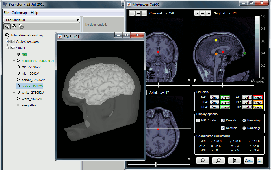
At the end of the process, make sure that the file "cortex_15000V" is selected (downsampled pial surface, that will be used for the source estimation). If it is not, double-click on it to select it as the default cortex surface. Do not worry about the big holes in the head surface, parts of MRI have been remove voluntarily for anonymization purposes.
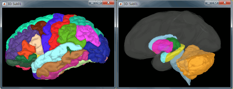
All the anatomical atlases generated by FreeSurfer were automatically imported: the cortical atlases (Desikan-Killiany, Mindboggle, Destrieux, Brodmann) and the sub-cortical regions (ASEG atlas).
Access the recordings
Link the recordings
We need to attach the continuous .fif files containing the recordings to the database.
- Switch to the "functional data" view.
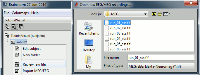
Right-click on the subject folder > Review raw file.
Select the file format: "MEG/EEG: Neuromag FIFF (*.fif)"
Select the first file in the MEG folder for subject 002: sub002/MEEG/run_01_sss.fif
Events: Ignore. We will read the stimulus triggers later.
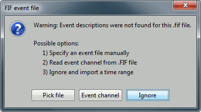
Refine registration now? NO
The head points that are available in the FIF files contain all the points that were digitized during the MEG acquisition, including the ones corresponding to the parts of the face that have been removed from the MRI. If we run the fitting algorithm, all the points around the nose will not match any close points on the head surface, leading to a wrong result. We will first remove the face points and then run the registration manually.
Channel classification
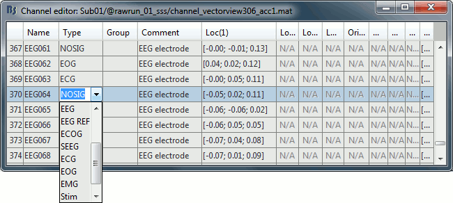
A few non-EEG channels are mixed in with the EEG channels, we need to change this before applying any operation on the EEG channels.
Right-click on the channel file > Edit channel file. Double-click on a cell to edit it.
Change the type of EEG062 to EOG (electrooculogram).
Change the type of EEG063 to ECG (electrocardiogram).
Change the type of EEG061 and EEG064 to NOSIG. Close the window and save the modifications.
MRI registration
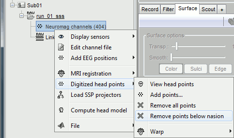
At this point, the registration MEG/MRI is based only on the three anatomical landmarks NAS/LPA/RPA. All the MRI scans were anonymized (defaced) and for some subjects the nasion could not be defined properly. We will try to refine this registration using the additional head points that were digitized (only the points above the nasion).
Right-click on the channel file > Digitized head points > Remove points below nasion.
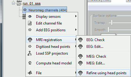
Right-click on the channel file > MRI registration > Refine using head points.
MEG/MRI registration, before (left) and after (right) this automatic registration procedure:
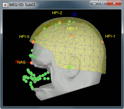
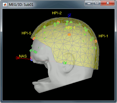
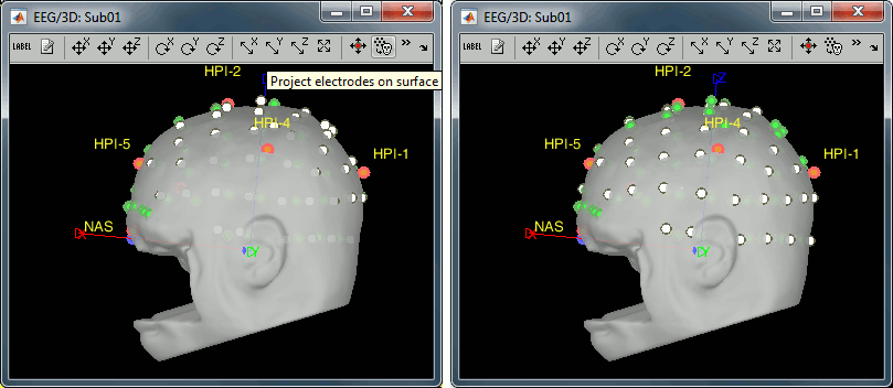
Right-click on the channel file > MRI registration > EEG: Edit...
Click on [Project electrodes on surface], then close the figure to save the modifications.
Read stimulus triggers
We need to read the stimulus markers from the STI channels. The following tasks can be done in an interactive way with menus in the Record tab, as in the introduction tutorials. We will illustrate here how to do this with the pipeline editor, it will be easier to batch it for all the runs and all the subjects.
- In Process1, select the "Link to raw file", click on [Run].
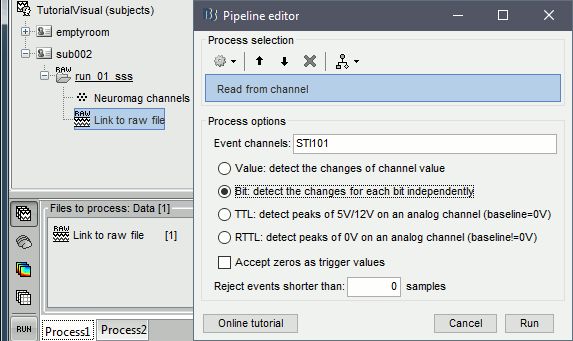
Select process Events > Read from channel, Channel: STI101, Detection mode: Bit.
Do not execute the process, we will add other processes to classify the markers.
- We want to create three categories of events, based on their numerical codes:
Famous faces: 5 (00101), 6 (00110), 7 (00111) => Bit 3 only
Unfamiliar faces: 13 (01101), 14 (01110), 15 (01111) => Bit 3 and 4
Scrambled images: 17 (10001), 18 (10010), 19 (10011) => Bit 5 only
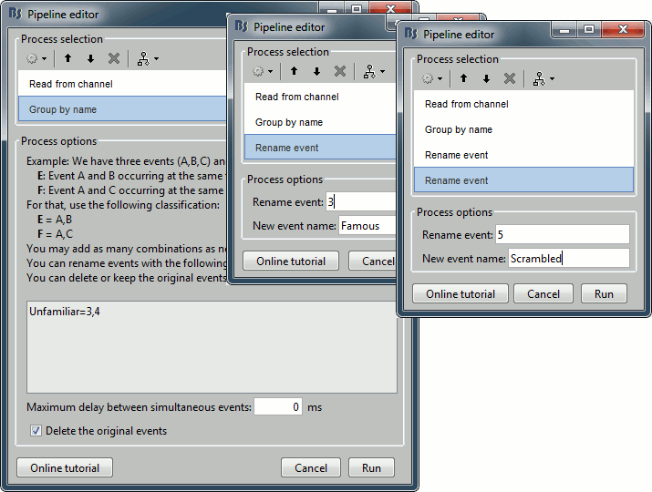
- We will start by creating the category "Unfamiliar" (combination of events "3" and "4") and remove the remove the initial events. Then we just have to rename the remaining "3" in "Famous", and all the "5" in "Scrambled".
Add process Events > Group by name: "Unfamiliar=3,4", Delay=0, Delete original events
Add process Events > Rename event: 3 => Famous
Add process Events > Rename event: 5 => Scrambled
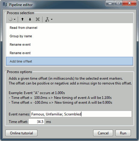
Add process Events > Add time offset to correct for the presentation delays:
Event names: "Famous, Unfamiliar, Scrambled", Time offset = 34.5ms
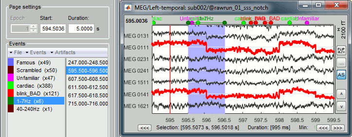
Finally run the script. Double-click on the recordings to make sure the labels were detected correctly. You can delete the unwanted events that are left in the recordings (1,2,9,13):

Pre-processing
Spectral evaluation
- Keep the "Link to raw file" in Process1.
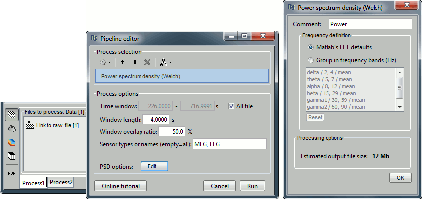
Run process Frequency > Power spectrum density (Welch) with the options illustrated below.
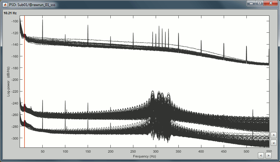
Right-click on the PSD file > Power spectrum.
The MEG sensors look awful, because of one small segment of data located around 248s. Open the MEG recordings and scroll to 248s (just before the first Unfamiliar event).
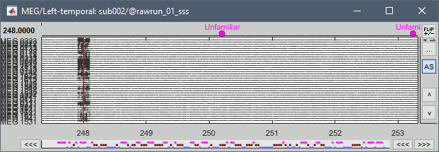
In these recordings, the continuous head tracking was activated, but it starts only at the time of the stimulation (248s) while the acquisition of the data starts 20s before (226s). The first 20s do not have head localization coils (HPI) coils activity and are not corrected by MaxFilter. After 248s, the HPI coils are on, and MaxFilter filters them out. The transition between the two states is not smooth and creates important distortions in the spectral domain. For a proper evaluation of the recordings, we should compute the PSD only after the HPI coils are turned on.
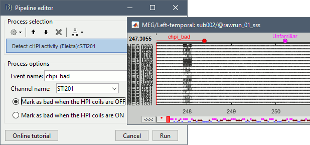
Run process Events > Detect cHPI activity (Elekta). This detects the changes in the cHPI activity from channel STI201 and marks all the data without head localization as bad.
Re-run the process Frequency > Power spectrum density (Welch). All the bad segments are excluded from the computation, therefore the PSD is now estimated only with the data after 248s.
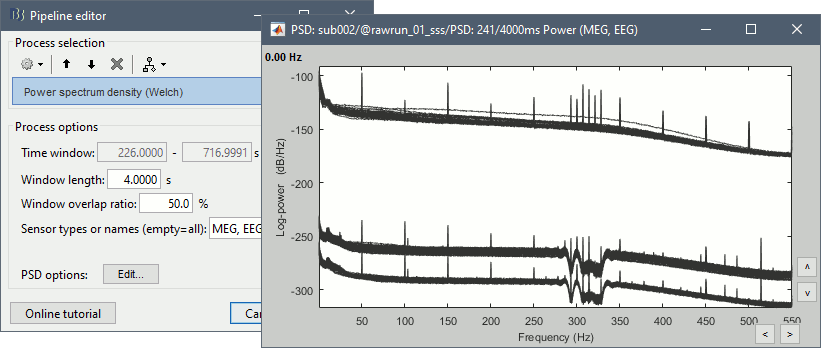
- Observations:
- Three groups of sensors, from top to bottom: EEG, MEG gradiometers, MEG magnetometers.
Power lines: 50 Hz and harmonics
- Alpha peak around 10 Hz
Artifacts due to Elekta electronics (HPI coils): 293Hz, 307Hz, 314Hz, 321Hz, 328Hz.
Peak from unknown source at 103.4Hz in the MEG only.
Suspected bad EEG channels: EEG016
- Close all the windows.
Remove line noise
- Keep the "Link to raw file" in Process1.
Select process Pre-process > Notch filter to remove the line noise (50-200Hz).
Add the process Frequency > Power spectrum density (Welch).
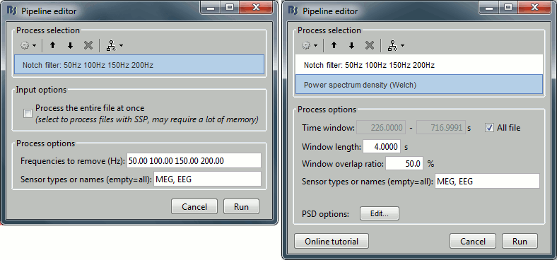
Double-click on the PSD for the new continuous file to evaluate the quality of the correction.
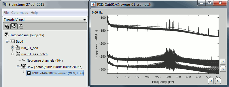
- Close all the windows (use the [X] button at the top-right corner of the Brainstorm window).
EEG reference and bad channels
Right-click on link to the processed file ("Raw | notch(50Hz ...") > EEG > Display time series.
Select channel EEG016 and mark it as bad (using the popup menu or pressing the Delete key).
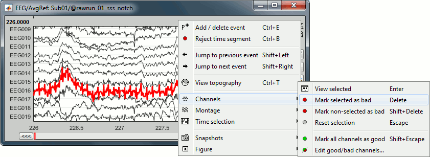
In the Record tab, menu Artifacts > Re-reference EEG > "AVERAGE".
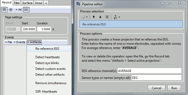
At the end, the window "select active projectors" is open to show the new re-referencing projector. Just close this window. To get it back, use the menu Artifacts > Select active projectors.
Artifact detection
Heartbeats: Detection
Empty the Process1 list (right-click > Clear list).
- Drag and drop the continuous processed file ("Raw | notch(50Hz...)") to the Process1 list.
Run process Events > Detect heartbeats: Channel name=EEG063, All file, Event name=cardiac
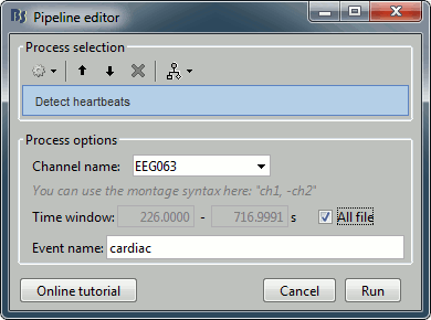
Eye blinks: Detection
- In many of the other tutorials, we detect the blinks and remove them with SSP. In this experiment, we are particularly interested in the subject's response to seeing the stimulus. Therefore we will exclude from the analysis all the recordings contaminated with blinks or other eye movements.
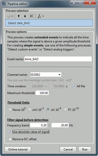
Run process Artifacts > Detect events above threshold:
Event name=blink_BAD, Channel=EEG062, All file, Maximum threshold=100, Threshold units=uV, Filter=[0.30,20.00]Hz, Use absolute value of signal.
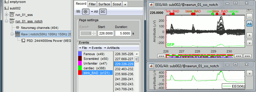
Inspect visually the two new cateogries of events: cardiac and blink_BAD.
- Close all the windows (using the [X] button).
Heartbeats: Correction with SSP
- Keep the "Raw | notch" file selected in Process1.
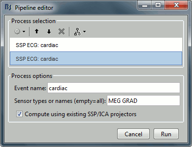
Select process Artifacts > SSP: Heartbeats > Sensor type: MEG MAG
Add process Artifacts > SSP: Heartbeats > Sensor type: MEG GRAD - Run the execution
Double-click on the continuous file to show all the MEG sensors.
In the Record tab, select sensors "Left-temporal".Menu Artifacts > Select active projectors.
In category cardiac/MEG MAG: Select component #1 and view topography.
In category cardiac/MEG GRAD: Select component #1 and view topography.

Make sure that selecting the two components removes the cardiac artifact. Then click [Save].
Additional bad segments
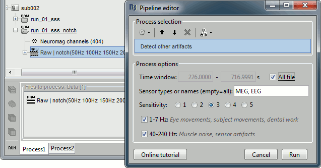
Process1>Run: Select the process "Events > Detect other artifacts". This should be done separately for MEG and EEG to avoid confusion about which sensors are involved in the artifact.
Display the MEG sensors. Review the segments that were tagged as artifact, determine if each event represents an artifact and then mark the time of the artifact as BAD. This can be done by selecting the time window around the artifact, then right-click > Reject time segment. Note that this detection process marks 1-second segments but the artifact can be shorter.

- Once all the events in the two categories are reviewed and bad segments are marked, the two categories (1-7Hz and 40-240Hz) can be deleted.
- Do this detection and review again for the EEG.
SQUID jumps
MEG signals recorded with Elekta-Neuromag systems frequently contain SQUID jumps (more information). These sharp steps followed by a change of baseline value are easy to identify visually but more complicated to detect automatically.
The process "Detect other artifacts" usually detects most of them in the category "1-7Hz". If you observe that some are skipped, you can try re-running it with a higher sensitivity. It is important to review all the sensors and all the time in each run to be sure these events are marked as bad segments.
Epoching and averaging
Import epochs
- Keep the "Raw | notch" file selected in Process1.
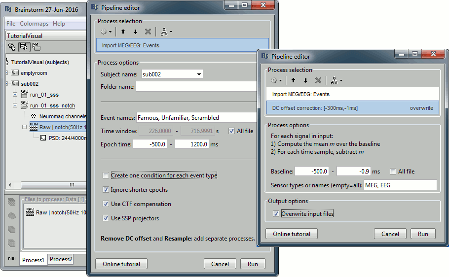
Select process: Import recordings > Import MEG/EEG: Events (do not run immediately)
Event names "Famous, Unfamiliar, Scrambled", All file, Epoch time=[-500,1200]msAdd process: Pre-process > Remove DC offset: Baseline=[-500,-0.9]ms - Run execution.
Average by run
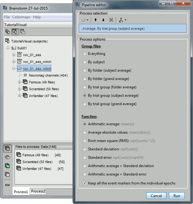
- In Process1, select all the imported trials.
Run process: Average > Average files: By trial groups (folder average)
Review EEG ERP
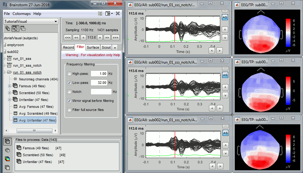
EEG evoked response (famous, scrambled, unfamiliar):
Open the Cluster tab and create a cluster with the channel EEG065 (button [NEW IND]).

Select the cluster, select the three average files, right-click > Clusters time series (Overlay:Files).
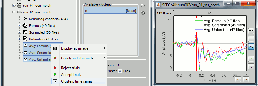
- Basic observations for EEG065 (right parieto-occipital electrode):
- Around 170ms (N170): greater negative deflection for Famous than Scrambled faces.
- After 250ms: difference between Famous and Unfamiliar faces.
Source estimation
MEG noise covariance: Empty room recordings
The minimum norm model we will use next to estimate the source activity can be improved by modeling the the noise contaminating the data. The section shows how to estimate the noise covariance in different ways for EEG and MEG. For the MEG recordings we will use the empty room measurements we have, and for the EEG we will compute it from the pre-stimulus baselines we have in all the imported epochs.
Create a new subject: emptyroom
Right-click on the new subject > Review raw file.
Select file: sample_group/emptyroom/090707_raw_st.fif
Do not apply default transformation, Ignore event channel.

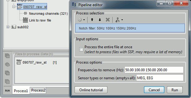
Select this new file in Process1 and run process Pre-process > Notch filter: 50 100 150 200Hz. When using empty room measurements to compute the noise covariance, they must be processed exactly in the same way as the other recordings.
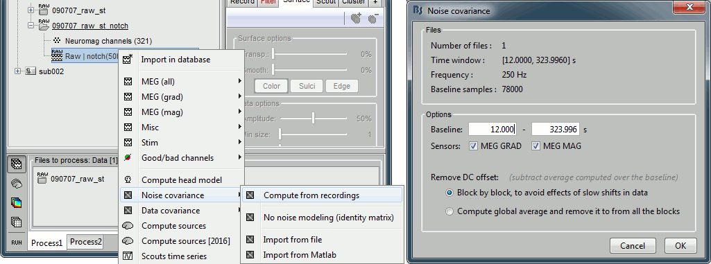
Right-click on the filtered noise recordings > Noise covariance > Compute from recordings:
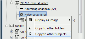
Right-click on the Noise covariance > Copy to other subjects
EEG noise covariance: Pre-stimulus baseline
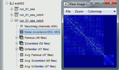
In folder sub002/run_01_sss_notch, select all the imported the imported trials, right-click > Noise covariance > Compute from recordings, Time=[-500,-0.9]ms, EEG only, Merge.
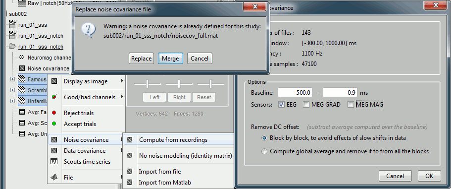
This computes the noise covariance only for EEG, and combines it with the existing MEG information.
BEM layers
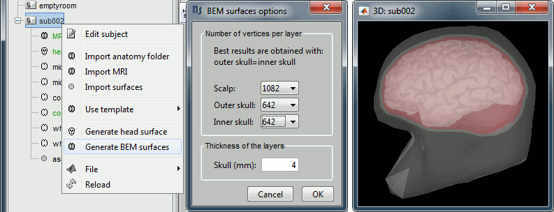
We will compute a BEM forward model to estimate the brain sources from the EEG recordings. For this, we need some layers defining the separation between the different tissues of the head (scalp, inner skull, outer skull).
- Go to the anatomy view (first button above the database explorer).
Right-click on the subject folder > Generate BEM surfaces: The number of vertices to use for each layer depends on your computing power and the accuracy you expect. You can try for instance with 1082 vertices (scalp) and 642 vertices (outer skull and inner skull).
Forward model: EEG and MEG
- Go back to the functional view (second button above the database explorer).
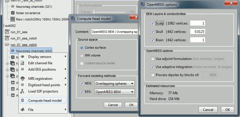
Model used: Overlapping spheres for MEG, OpenMEEG BEM for EEG (more information).
In folder sub002/run_01_sss_notch, right-click on the channel file > Compute head model.
Keep all the default options . Expect this to take a while...
Inverse model: Minimum norm estimates
Right-click on the new head model > Compute sources [2016]: MEG MAG + GRAD (default options)
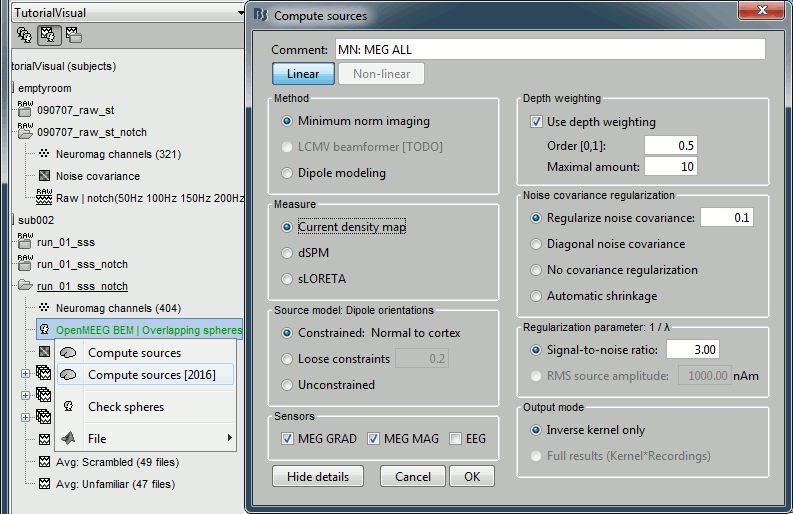
Right-click on the new head model > Compute sources [2016]: EEG (default bad channels).
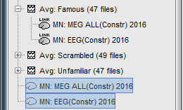
At the end we have two inverse operators, that are shared for all the files of the run (single trials and averages). If we wanted to look at the run-level source averages, we could normalize the source maps with a Z-score wrt baseline. In this tutorial, we will first average across runs and normalize the subject-level averages. This will be done in the next tutorial (group analysis).
Time-frequency analysis
We will compute the time-frequency decomposition of each trial using Morlet wavelets, and average the power of the Morlet coefficients for each condition and each run separately. We will restrict the computation to the MEG magnetometers and the EEG channels to limit the computation time and disk usage.
- In Process1, select the imported trials "Famous" for run#01.
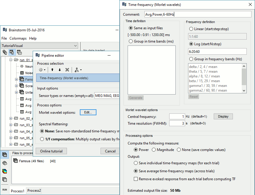
Run process Frequency > Time-frequency (Morlet wavelets): Sensor types=MEG MAG,EEG
Not normalized, Frequency=Log(6:20:60), Measure=Power, Save average
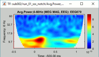
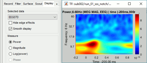
Double-click on the file to display it. In the Display tab, select the option "Hide edge effects" to exclude form the display all the values that could not be estimated in a reliable way. Let's extract only the good values from this file (-200ms to +900ms).
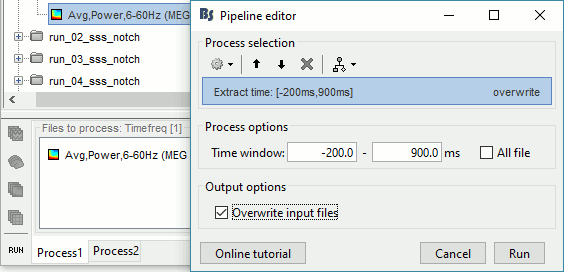
- In Process1, select the time-frequency file.
Run process Extract > Extract time: Time window=[-200, 900]ms, Overwrite input files
Display the file again, observe that all the possibly bad values are gone.
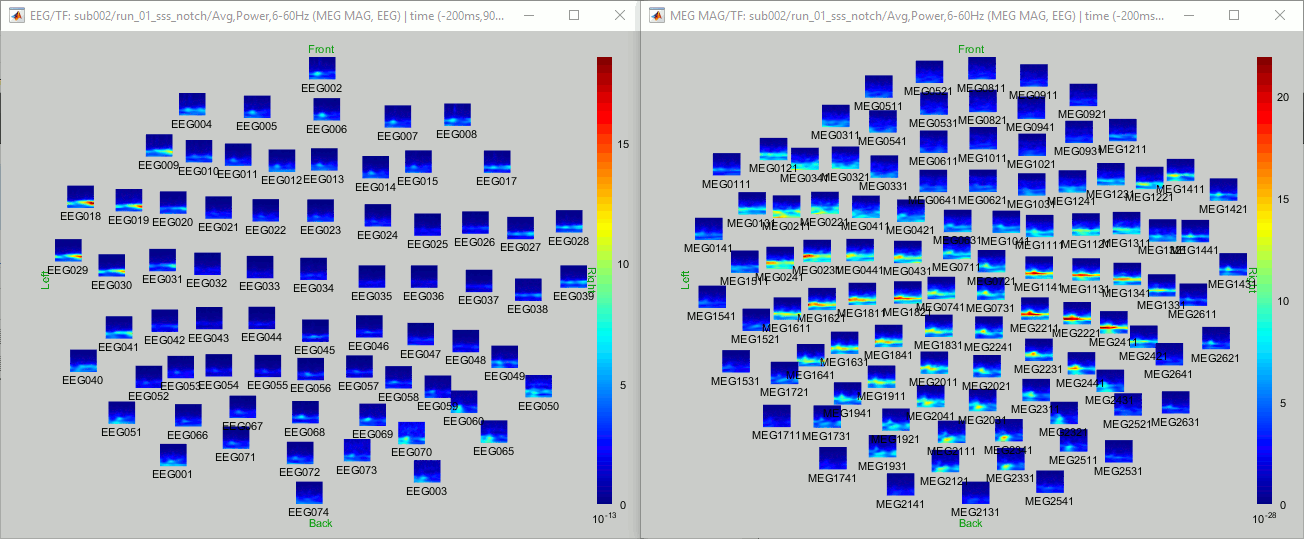
You can display all the sensors at once (MEG MAG or EEG): right-click > 2D Layout (maps).
- Repeat these steps for other conditions (Scrambled and Unfamiliar) and the other runs (2-6). There is no way with this process to compute all the averages at once, as we did with the process "Average files". This will be easier to run from a script.
- If we wanted to look at the run-level source averages, we could normalize these time-frequency maps. In this tutorial, we will first average across runs and normalize the subject-level averages. This will be done in the next tutorial (group analysis).
Scripting
We have now all the files we need for the group analysis (next tutorial). We need to repeat the same operations for all the runs and all the subjects. Some of these steps are fully automatic and take a lot of time (filtering, computing the forward model), they should be executed from a script.
However, we recommend you always review manually some of the pre-processing steps (selection of the bad segments and bad channels, SSP/ICA components). Do not trust blindly any fully automated cleaning procedure.
For the strict reproducibility of this analysis, we provide a script that processes all the 19 subjects: brainstorm3/toolbox/script/tutorial_visual_single.m (execution time: 10-30 hours)
Report for the first subject: report_TutorialVisual_sub001.html
You should note that this is not the result of a fully automated procedure. The bad channels were identified manually and are defined for each run in the script. The bad segments were detected automatically, confirmed manually for each run and saved in external files distributed with the Brainstorm package sample_group_freesurfer.zip (sample_group/brainstorm/bad_segments/*.mat).
All the process calls (bst_process) were generated automatically using with the script generator (menu Generate .m script in the pipeline editor). Everything else was added manually (loops, bad channels, file copies).
Bad subjects
After evaluating the results for the 19 subjects, 3 subjects were excluded from the analysis:
sub001: Error during the digitization of the EEG electrodes with the Polhemus (the same electrode was clicked twice). This impacts only the EEG, this subject could be used for MEG analysis.
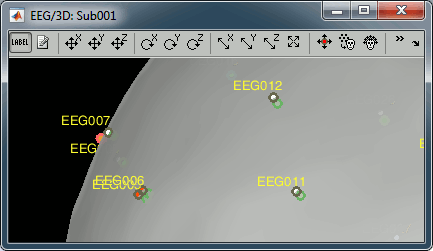
sub005: Too many blinks or other eye movements.
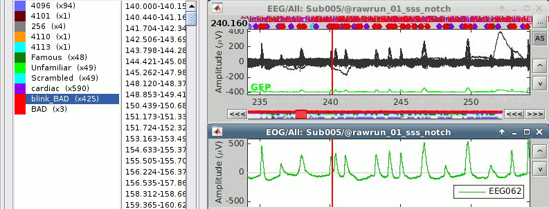
sub016: Too many blinks or other eye movements.
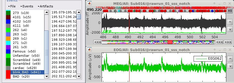
Make sure you don't include these subjects in the group analysis.

