|
Size: 1430
Comment:
|
Size: 17341
Comment:
|
| Deletions are marked like this. | Additions are marked like this. |
| Line 1: | Line 1: |
| = Tutorial 13: Head model = ''Authors: Francois Tadel, Elizabeth Bock, John C Mosher, Sylvain Baillet'' |
= Tutorial 20: Head model = ''Authors: Francois Tadel, Elizabeth Bock, John C Mosher, Richard Leahy, Sylvain Baillet'' |
| Line 4: | Line 4: |
| <<TableOfContents(2,2)>> | The following tutorials describe how the brain activity can be estimated from the MEG/EEG recordings we have processed until now. This process consists in solving two separate problems: the modeling of the electromagnetic properties of the head ('''head model''' or '''forward model''') and the inversion of this model. This tutorial will explain how to compute a head model for the subject of our auditory oddball experiment. Its scope is limited to linear distributed source models (there is no dipole fitting available in the software). '' '' |
| Line 6: | Line 6: |
| From continuous tutorials: | <<TableOfContents(2,2)>> '' '' |
| Line 8: | Line 8: |
| == Source analysis == Let's reproduce the same observations at the source level. The concepts related with the source estimation are not discussed here; for more information, refer to the introduction tutorials #6 to #8. |
<<TAG(Advanced)>> '' '' |
| Line 11: | Line 10: |
| First, '''delete''' all the files related with the source estimation calculated in the previous tutorials, available in the ''(Common files)'' folder: the head model, the noise covariance and inverse model. We can now provide a better estimate of the noise (affects the inverse model), and we defined new SSP operators (affects the head model). | == Why estimating sources? == Reconstructing the activity of the brain from MEG or EEG recordings can be a difficult and long process. We tried to make it as automatic as possible, but you have to understand its advantages and issues before deciding if it can bring anything to your study. '' '' |
| Line 13: | Line 13: |
| === Head model === Right-click on any node that contains the channel file (including the channel file itself), and select: "'''Compute head model'''". Leave all the default options: cortex source space, and overlapping spheres. The lead field matrix is saved in file "Overlapping spheres" in ''(Common files)''. |
The primary objective is to '''localize''' the regions of the brain that generated our signals of interest. From the sensor topographies in MEG and EEG, we can have a general idea of where the signal generators are located, but we cannot be more precise than identifying the hemisphere or the lobe. Using source estimation methods, we can expect to get a spatial resolution in the range of the centimeter, or even a few millimeters in the good cases. '' '' |
| Line 16: | Line 15: |
| {{http://neuroimage.usc.edu/brainstorm/Tutorials/TutRawAvg?action=AttachFile&do=get&target=forward.gif|forward.gif|class="attachment"}} | While localizing the signals, we can also expect some form of '''deconvolution''' of our signals. In EEG, the scalp topographies are very smooth and it is common to have different effects that are superimposed in the signals recorded by most of the electrodes. Moving to the source space may help separating the sources and obtain cleaner and unmixed signals. '' '' |
| Line 18: | Line 17: |
| Specifically for '''MEG''', working in source space solves many of the problems associated with this modality. The subject's head is not fixed in an MEG system, so it has a great chance of moving during the experiment. Also, the position of the sensors do not adapt to the shape and size of the head. Therefore between two acquisition runs, or between subjects with different morphologies, there is a high chance that '''the same MEG sensor records different parts of the brain'''. This problem does not exist in EEG, where the electrodes are in standard positions and follow the subject in all the movements. '' '' | |
| Line 19: | Line 19: |
| Another point that makes '''MEG signals difficult to review''' is the variability in the sensors. Every manufacturer uses different types of sensors, that are sensitive to different orientations and distances, and that produce signals with different shapes. Again, this is not a problem in EEG: the only variability you can get between two EEG systems is the level of noise and the ease of use of the cap, but the signals will look very similar. Projecting all the data on the individual brains addresses these last two issues. '' '' | |
| Line 20: | Line 21: |
| <<EmbedContent("http://neuroimage.usc.edu/bst/get_prevnext.php?prev=Tutorials/ExploreRecordings&next=Tutorials/NoiseCovariance")>> | However, if your interest is only in the latency of an event, in detecting the lateralization of a known effect or in training blindly a classifier, you might not be interested in these complicated models that multiply by 50 the size of your files. Go for fancy methods only when you think they can bring some added value to your analysis, not because everybody around uses them. '' '' |
| Line 22: | Line 23: |
| <<EmbedContent(http://neuroimage.usc.edu/bst/get_feedback.php?Tutorials/HeadModel)>> | <<TAG(Advanced)>> '' '' == The origins of the MEG/EEG signals == To understand how we are reconstructing the sources, it is interesting to have an idea of the physiological origins of MEG and EEG signals. The models we use are based on some physiological assumptions that are not always valid, understanding them may help you in selecting the appropriate method. '' '' It is assumed that most of the currents we record are related with the postsynaptic activity of the pyramidal neurons in the cerebral cortex. These cells are '''aligned spatially''' and '''perpendicular to the cortex surface'''. Millions of post-synaptic potentials in the apical dendrites of neighbouring pyramidal neurons sum up in time and space to form what we can approximate at a macroscopic level with a few electric dipoles (green arrows below). '' '' The primary and volume currents generated by these dipoles create a potential distribution and a magnetic field at the surface of the head. We can record them with bipolar montages of electrodes placed on the skin (EEG) or very sensitive superconducting detectors (SQUIDs/MEG). '' '' . {{attachment:origins.gif||height="342",width="538"}} '' '' . <<HTML(<div align="right"><FONT size="-1" color="#CCCCCC"><I>Matti Hamalainen, 2007</I></FONT></div>)>> '' '' <<TAG(Advanced)>> '' '' == Source space == '''Dipole fitting vs distributed methods''' '' '' The source estimation process consists in estimating the position and activity of a set of electric dipoles, to approximate the activity of the brain that produced the MEG/EEG data we recorded. Two families of solutions were explored in the past decades: the '''dipole fitting methods''' (we estimate the position and amplitude of a very limited number of dipoles over short time windows) and the '''distributed methods''' (we define a priori a dense grid of dipoles and then estimate their activity from the recordings). '' '' The single dipole fitting approaches are very efficient in specific cases were we know in advance the number or regions involved and their latencies of activity. But they are difficult to generalize and automate, and not adapted for group analysis. With Brainstorm, we decided to work only with distributed source models, which require less manual tuning for getting acceptable results. '' '' '''Location constraints''' '' '' Our first step of modeling consists in defining the '''positions and orientations of the dipoles''' for which we want to estimate the activity. This set of dipoles is our '''source space'''. By default, we limit our analysis to the '''cortex envelope''', based on this observation that most of the MEG/EEG signals is related with the synchronous activity of assemblies or cortical pyramidal cells. The simple solution we recommend is to use directly the vertices of the cortical surface we imported in the first tutorials (the nodes we can see in the grey mesh in the left image below). '' '' In order to represent all the possible dipole orientations, we define '''three dipoles for each vertex''' of the cortex surface, corresponding to three orthogonal directions (X,Y,Z). When importing the anatomy of the subject, we downsampled the cortex surface to '''15,000 vertices'''. This will correspond to a source space of '''45,000 dipoles'''. We will compute a forward model that connects the activity of these 45,000 dipoles with the 275 MEG sensors we have in this dataset. '' '' This default number of 15,000 vertices is empirical. Over the years, our experience seemed to show that it represents a good balance between the representation of the brain circumvolutions, the surface sampling and the amount of data that is generated. Using less vertices makes it difficult to preserve the shape of the brain, using more vertices produces more data without adding to the spatial resolution of the method and may lead to memory issues. '' '' '''Orientation constraints''' '' '' Additionally, we can impose '''constraints of orientation''' on the dipoles, to match the physiological observation that the pyramidal cells are mostly organized perpendicularly to the cortex surface. This has the advantage of limiting the number of dipoles to 15,000 (one per vertex) and making the results much easier to display and process. However, this constraint is most of the time too strong and distorts the reconstruction. This orientation constraint is an option of the inverse model and will be discussed in the following introduction tutorials. '' '' '''Fully unconstrained''' '' '' The spatial constraint of imposing all the dipoles to be on the cortical surface might also be too restrictive in some cases, because our model is then not able to represent correctly the activity in deeper brain structures or in the cerebellum. Therefore we also offer an option to use the '''entire brain volume''' as our source space (the green dots below represent dipoles locations in volume model). This produces results that can be better or worse depending on the data, but in all the cases much more difficult to review. Volume and mixed head volumes are discussed in the advanced tutorials about source modeling. '' '' . {{attachment:source_space.gif||height="200",width="243"}} {{attachment:source_volume.gif||height="200",width="255"}} '' '' <<TAG(Advanced)>> '' '' == Forward problem == The first step of the source reconstruction consists in computing a model that explains how the electric currents or the magnetic fields flow from the electric generators in the brain (source space) through the different tissues of the head (mostly brain, CSF, skull and skin), to finally reach the sensors. '' '' * The question of building a model that connects the values we observe outside of the head (MEG/EEG) to the electric activity of the cortical dipoles in the brain is called '''forward problem'''. '' '' * The model we obtain after solving this problem is called '''head model''' in Brainstorm, but can also be referred to as '''forward model''', '''leadfield matrix''' or '''gain matrix'''. '' '' * In this tutorial we will use the default source space: the low-resolution cortex surface with 15,000 vertices, as the support of 45,000 dipoles. We will use indifferently the terms '''dipole''' and '''source'''. '' '' * What we expect to get at the end of this process is a matrix '''[Nsensors x Nsources]'''. <<BR>><<BR>> {{attachment:forward_inverse.gif}} '' '' ==== Available methods for MEG forward modeling ==== * '''Single sphere''': The head is considered as a homogeneous sphere. '' '' * '''Overlapping spheres''': Refines the previous model by fitting one local sphere for each sensor. '' '' * '''OpenMEEG BEM''': Symmetric Boundary Element Method from the open-source software OpenMEEG. Described in an advanced tutorial: [[Tutorials/TutBem|BEM head model]]. '' '' ==== Models recommended for each modality ==== * '''MEG''': Overlapping spheres.<<BR>>The magnetic fields are not too much affected by the heterogeneity of the tissues of the head. There is no real need for modeling the head with too much details. '' '' * '''EEG''': OpenMEEG BEM.<<BR>>The electric currents are strongly affected by jumps between very conductive tissues (brain, CSF, skin) and an isolant medium (the skull). A realistic head model is advised for integrating the properties of the skull correctly. When computing a BEM model is not an option, for instance if OpenMEEG crashes for unknown reasons, the Berg's three-layer sphere can be an acceptable option. '' '' * '''sEEG/ECoG''': The OpenMEEG BEM option is the only one available. '' '' == Computation == The forward models are related with the anatomy of the subject and the description of the sensors, therefore the menus associated to its computation are attached to the channel file. '' '' * In the imported '''Run#01''', right-click on the channel file or the folder > '''Compute head model'''. <<BR>>Keep the default options selected: Source space='''Cortex''', Forward model='''Overlapping spheres'''.<<BR>><<BR>> {{attachment:compute_popup.gif||height="161",width="254"}} {{attachment:compute_options.gif||height="247",width="211"}} '' '' * You obtain one new file in the database. It is always saved in the same folder as the channel file.<<BR>>There is not much you can do with this file except for using it for estimating sources. This will be the purpose of the following tutorials. '' '' * Right-click on the new head model > ''Check spheres''. This window shows the spheres that were estimated. You can check them by following the indications written in green at the bottom of the window: use left/right arrows. At each step, the current sensor marker is displayed in red, and the sphere you see is its local estimation of the inner skull shape. <<BR>><<BR>> {{attachment:headmodel_popup.gif||height="124",width="258"}} {{attachment:headmodel_spheres.gif||height="181",width="272"}} '' '' * This algorithm is supposed to use the inner skull surface from the subject, but we usually do not have this information. In this case, a pseudo-innerskull is reconstructed using a dilated version of the cortex envelope. '' '' Repeat the same operation for the other file. We have two different acquisition runs with two different relative position of the head and the sensors, therefore we need to compute two different head models. '' '' * In the imported '''Run#02''', right-click on the channel file > '''Compute head model'''. <<BR>><<BR>> {{attachment:run02_popup.gif||height="220",width="265"}} {{attachment:run02_files.gif||height="220",width="193"}} '' '' <<TAG(Advanced)>> '' '' == Database explorer == Additional considerations about the management of the head model files. '' '' * If you have '''multiple head models''' computed in the same folder, you would see one displayed in green and the others in black. The one in green is selected as the default head model, it will be used for all the following computation steps. To change the default selection, double-click on another head model file (or right-click > Set as default head model). '' '' * You can use the database explore for '''batching the computation''' of the head model. The menu "Compute head model" is available in popup menus in the database explorer at all the levels. It is applied recursively to all the folders contained in the node(s) you selected. '' '' <<TAG(Advanced)>> '' '' == On the hard drive == Right-click on any head model > File > View file contents: '' '' . {{attachment:headmodel_contents.gif||height="440",width="486"}} '' '' ==== Structure of the head model files ==== * '''MEGMethod''': Forward model used for MEG sensors ('os_meg', 'meg_sphere', 'openmeeg' or empty). '' '' * '''EEGMethod''': Forward model used for EEG sensors ('eeg_3sphereberg', 'openmeeg' or empty). '' '' * '''ECOGMethod''': Forward model used for ECoG sensors ('openmeeg' or empty). '' '' * '''SEEGMethod''': Forward model used for sEEG sensors ('openmeeg' or empty). '' '' * '''Gain''': Leadfield matrix, [Nsensors x Nsources], equivalent to [Nsensors x 3*Nvertices] '' '' * '''Comment''': String displayed in the database explorer to represent this file. '' '' * '''HeadModelType''': Type of source space used for this head model ('surface', 'volume', 'mixed'). '' '' * '''GridLoc''': [Nvertices x 3], (x,y,z) positions of the grid of source points. In the case of a surface head model, it corresponds to a copy of the 'Vertices' matrix from the cortex surface file. '' '' * '''GridOrient''': [Nvertices x 3], direction of the normal to the surface for each vertex point (copy of the 'VertNormals' matrix of the cortex surface). Empty in the case of a volume head model. '' '' * '''GridAtlas''': In the case of mixed head models, contains a copy of the "Source model options" atlas structure that was used for creating the model. '' '' * '''SurfaceFile''': Relative path to the cortex surface file related with this head model. '' '' * '''Param''': Description of the sphere that was estimated for each sensor (Center/Radius).<<BR>> '' '' '''Gain matrix''' '' '' * The Gain matrix stores the leadfield for 3 orientations (x,y,z) at each grid point (p1, p2, ...). <<BR>>The successive columns of the Gain matrix are: ['''p1'''_x, '''p1'''_y, '''p1'''_z, p2_x, p2_y, p2_z ...] '' '' * To convert this unconstrained leadfield matrix to a '''constrained model''', where the orientation of each dipole is fixed and normal to the cortex surface: '' '' * Export the head model file to the HeadModel structure: Right-click > File > '''Export to Matlab'''. '' '' * > Gain_constrained = '''bst_gain_orient'''(HeadModel.Gain, HeadModel.GridOrient); '' '' * The dimension of the output matrix is three times smaller: [Nsensors x Nvertices] '' '' == References == * Huang MX, Mosher JC, Leahy RM (1999)<<BR>>"A sensor-weighted overlapping-sphere head model and exhaustive head model comparison for MEG," Phys Med Biol, 44:423-440 | [[http://neuroimage.usc.edu/paperspdf/PMB99.pdf|pdf]] '' '' == Additional documentation == * Tutorial: [[Tutorials/TutBem|BEM with OpenMEEG]] '' '' * Tutorial: [[Tutorials/TutVolSource|Volume source estimation]] '' '' * Forum: Sensor modeling: http://neuroimage.usc.edu/forums/showthread.php?1295 '' '' * Forum: EEG reference: http://neuroimage.usc.edu/forums/showthread.php?1525#post6718 '' '' * Forum: EEG and default anatomy: http://neuroimage.usc.edu/forums/showthread.php?1774 '' '' * Forum: Mixed head models indices: http://neuroimage.usc.edu/forums/showthread.php?1878 '' '' <<HTML(<!-- END-PAGE -->)>> '' '' <<EmbedContent("http://neuroimage.usc.edu/bst/get_prevnext.php?prev=Tutorials/ChannelClusters&next=Tutorials/NoiseCovariance")>> '' '' <<EmbedContent(http://neuroimage.usc.edu/bst/get_feedback.php?Tutorials/HeadModel)>> '' '' |
Tutorial 20: Head model
Authors: Francois Tadel, Elizabeth Bock, John C Mosher, Richard Leahy, Sylvain Baillet
The following tutorials describe how the brain activity can be estimated from the MEG/EEG recordings we have processed until now. This process consists in solving two separate problems: the modeling of the electromagnetic properties of the head (head model or forward model) and the inversion of this model. This tutorial will explain how to compute a head model for the subject of our auditory oddball experiment. Its scope is limited to linear distributed source models (there is no dipole fitting available in the software).
Contents
Why estimating sources?
Reconstructing the activity of the brain from MEG or EEG recordings can be a difficult and long process. We tried to make it as automatic as possible, but you have to understand its advantages and issues before deciding if it can bring anything to your study.
The primary objective is to localize the regions of the brain that generated our signals of interest. From the sensor topographies in MEG and EEG, we can have a general idea of where the signal generators are located, but we cannot be more precise than identifying the hemisphere or the lobe. Using source estimation methods, we can expect to get a spatial resolution in the range of the centimeter, or even a few millimeters in the good cases.
While localizing the signals, we can also expect some form of deconvolution of our signals. In EEG, the scalp topographies are very smooth and it is common to have different effects that are superimposed in the signals recorded by most of the electrodes. Moving to the source space may help separating the sources and obtain cleaner and unmixed signals.
Specifically for MEG, working in source space solves many of the problems associated with this modality. The subject's head is not fixed in an MEG system, so it has a great chance of moving during the experiment. Also, the position of the sensors do not adapt to the shape and size of the head. Therefore between two acquisition runs, or between subjects with different morphologies, there is a high chance that the same MEG sensor records different parts of the brain. This problem does not exist in EEG, where the electrodes are in standard positions and follow the subject in all the movements.
Another point that makes MEG signals difficult to review is the variability in the sensors. Every manufacturer uses different types of sensors, that are sensitive to different orientations and distances, and that produce signals with different shapes. Again, this is not a problem in EEG: the only variability you can get between two EEG systems is the level of noise and the ease of use of the cap, but the signals will look very similar. Projecting all the data on the individual brains addresses these last two issues.
However, if your interest is only in the latency of an event, in detecting the lateralization of a known effect or in training blindly a classifier, you might not be interested in these complicated models that multiply by 50 the size of your files. Go for fancy methods only when you think they can bring some added value to your analysis, not because everybody around uses them.
The origins of the MEG/EEG signals
To understand how we are reconstructing the sources, it is interesting to have an idea of the physiological origins of MEG and EEG signals. The models we use are based on some physiological assumptions that are not always valid, understanding them may help you in selecting the appropriate method.
It is assumed that most of the currents we record are related with the postsynaptic activity of the pyramidal neurons in the cerebral cortex. These cells are aligned spatially and perpendicular to the cortex surface. Millions of post-synaptic potentials in the apical dendrites of neighbouring pyramidal neurons sum up in time and space to form what we can approximate at a macroscopic level with a few electric dipoles (green arrows below).
The primary and volume currents generated by these dipoles create a potential distribution and a magnetic field at the surface of the head. We can record them with bipolar montages of electrodes placed on the skin (EEG) or very sensitive superconducting detectors (SQUIDs/MEG).
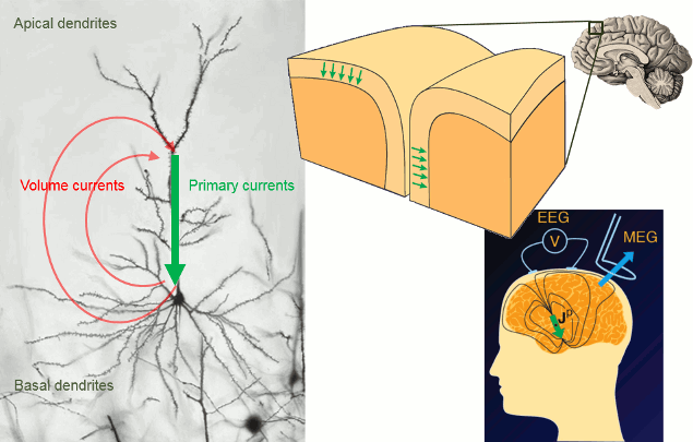
- Matti Hamalainen, 2007
Source space
Dipole fitting vs distributed methods
The source estimation process consists in estimating the position and activity of a set of electric dipoles, to approximate the activity of the brain that produced the MEG/EEG data we recorded. Two families of solutions were explored in the past decades: the dipole fitting methods (we estimate the position and amplitude of a very limited number of dipoles over short time windows) and the distributed methods (we define a priori a dense grid of dipoles and then estimate their activity from the recordings).
The single dipole fitting approaches are very efficient in specific cases were we know in advance the number or regions involved and their latencies of activity. But they are difficult to generalize and automate, and not adapted for group analysis. With Brainstorm, we decided to work only with distributed source models, which require less manual tuning for getting acceptable results.
Location constraints
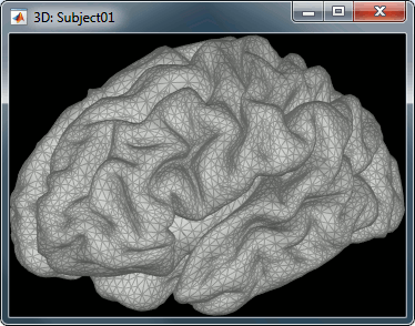
Our first step of modeling consists in defining the positions and orientations of the dipoles for which we want to estimate the activity. This set of dipoles is our source space. By default, we limit our analysis to the cortex envelope, based on this observation that most of the MEG/EEG signals is related with the synchronous activity of assemblies or cortical pyramidal cells. The simple solution we recommend is to use directly the vertices of the cortical surface we imported in the first tutorials (the nodes we can see in the grey mesh in the left image below).
In order to represent all the possible dipole orientations, we define three dipoles for each vertex of the cortex surface, corresponding to three orthogonal directions (X,Y,Z). When importing the anatomy of the subject, we downsampled the cortex surface to 15,000 vertices. This will correspond to a source space of 45,000 dipoles. We will compute a forward model that connects the activity of these 45,000 dipoles with the 275 MEG sensors we have in this dataset.
This default number of 15,000 vertices is empirical. Over the years, our experience seemed to show that it represents a good balance between the representation of the brain circumvolutions, the surface sampling and the amount of data that is generated. Using less vertices makes it difficult to preserve the shape of the brain, using more vertices produces more data without adding to the spatial resolution of the method and may lead to memory issues.
Orientation constraints
Additionally, we can impose constraints of orientation on the dipoles, to match the physiological observation that the pyramidal cells are mostly organized perpendicularly to the cortex surface. This has the advantage of limiting the number of dipoles to 15,000 (one per vertex) and making the results much easier to display and process. However, this constraint is most of the time too strong and distorts the reconstruction. This orientation constraint is an option of the inverse model and will be discussed in the following introduction tutorials.
Fully unconstrained
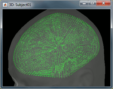
The spatial constraint of imposing all the dipoles to be on the cortical surface might also be too restrictive in some cases, because our model is then not able to represent correctly the activity in deeper brain structures or in the cerebellum. Therefore we also offer an option to use the entire brain volume as our source space (the green dots below represent dipoles locations in volume model). This produces results that can be better or worse depending on the data, but in all the cases much more difficult to review. Volume and mixed head volumes are discussed in the advanced tutorials about source modeling.
Forward problem
The first step of the source reconstruction consists in computing a model that explains how the electric currents or the magnetic fields flow from the electric generators in the brain (source space) through the different tissues of the head (mostly brain, CSF, skull and skin), to finally reach the sensors.
The question of building a model that connects the values we observe outside of the head (MEG/EEG) to the electric activity of the cortical dipoles in the brain is called forward problem.
The model we obtain after solving this problem is called head model in Brainstorm, but can also be referred to as forward model, leadfield matrix or gain matrix.
In this tutorial we will use the default source space: the low-resolution cortex surface with 15,000 vertices, as the support of 45,000 dipoles. We will use indifferently the terms dipole and source.
What we expect to get at the end of this process is a matrix [Nsensors x Nsources].

Available methods for MEG forward modeling
Single sphere: The head is considered as a homogeneous sphere.
Overlapping spheres: Refines the previous model by fitting one local sphere for each sensor.
OpenMEEG BEM: Symmetric Boundary Element Method from the open-source software OpenMEEG. Described in an advanced tutorial: BEM head model.
Models recommended for each modality
MEG: Overlapping spheres.
The magnetic fields are not too much affected by the heterogeneity of the tissues of the head. There is no real need for modeling the head with too much details.EEG: OpenMEEG BEM.
The electric currents are strongly affected by jumps between very conductive tissues (brain, CSF, skin) and an isolant medium (the skull). A realistic head model is advised for integrating the properties of the skull correctly. When computing a BEM model is not an option, for instance if OpenMEEG crashes for unknown reasons, the Berg's three-layer sphere can be an acceptable option.sEEG/ECoG: The OpenMEEG BEM option is the only one available.
Computation
The forward models are related with the anatomy of the subject and the description of the sensors, therefore the menus associated to its computation are attached to the channel file.
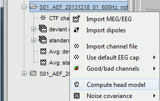
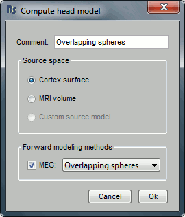
In the imported Run#01, right-click on the channel file or the folder > Compute head model.
Keep the default options selected: Source space=Cortex, Forward model=Overlapping spheres.
You obtain one new file in the database. It is always saved in the same folder as the channel file.
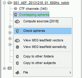
There is not much you can do with this file except for using it for estimating sources. This will be the purpose of the following tutorials.Right-click on the new head model > Check spheres. This window shows the spheres that were estimated. You can check them by following the indications written in green at the bottom of the window: use left/right arrows. At each step, the current sensor marker is displayed in red, and the sphere you see is its local estimation of the inner skull shape.
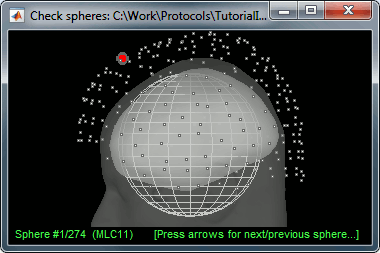
This algorithm is supposed to use the inner skull surface from the subject, but we usually do not have this information. In this case, a pseudo-innerskull is reconstructed using a dilated version of the cortex envelope.
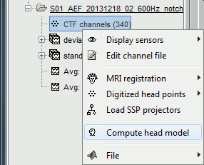
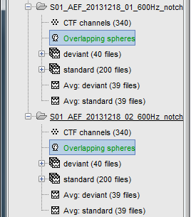
Repeat the same operation for the other file. We have two different acquisition runs with two different relative position of the head and the sensors, therefore we need to compute two different head models.
In the imported Run#02, right-click on the channel file > Compute head model.
Database explorer
Additional considerations about the management of the head model files.
If you have multiple head models computed in the same folder, you would see one displayed in green and the others in black. The one in green is selected as the default head model, it will be used for all the following computation steps. To change the default selection, double-click on another head model file (or right-click > Set as default head model).
You can use the database explore for batching the computation of the head model. The menu "Compute head model" is available in popup menus in the database explorer at all the levels. It is applied recursively to all the folders contained in the node(s) you selected.
On the hard drive
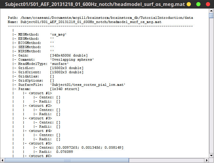
Right-click on any head model > File > View file contents:
Structure of the head model files
MEGMethod: Forward model used for MEG sensors ('os_meg', 'meg_sphere', 'openmeeg' or empty).
EEGMethod: Forward model used for EEG sensors ('eeg_3sphereberg', 'openmeeg' or empty).
ECOGMethod: Forward model used for ECoG sensors ('openmeeg' or empty).
SEEGMethod: Forward model used for sEEG sensors ('openmeeg' or empty).
Gain: Leadfield matrix, [Nsensors x Nsources], equivalent to [Nsensors x 3*Nvertices]
Comment: String displayed in the database explorer to represent this file.
HeadModelType: Type of source space used for this head model ('surface', 'volume', 'mixed').
GridLoc: [Nvertices x 3], (x,y,z) positions of the grid of source points. In the case of a surface head model, it corresponds to a copy of the 'Vertices' matrix from the cortex surface file.
GridOrient: [Nvertices x 3], direction of the normal to the surface for each vertex point (copy of the 'VertNormals' matrix of the cortex surface). Empty in the case of a volume head model.
GridAtlas: In the case of mixed head models, contains a copy of the "Source model options" atlas structure that was used for creating the model.
SurfaceFile: Relative path to the cortex surface file related with this head model.
Param: Description of the sphere that was estimated for each sensor (Center/Radius).
Gain matrix
The Gain matrix stores the leadfield for 3 orientations (x,y,z) at each grid point (p1, p2, ...).
The successive columns of the Gain matrix are: [p1_x, p1_y, p1_z, p2_x, p2_y, p2_z ...]To convert this unconstrained leadfield matrix to a constrained model, where the orientation of each dipole is fixed and normal to the cortex surface:
Export the head model file to the HeadModel structure: Right-click > File > Export to Matlab.
> Gain_constrained = bst_gain_orient(HeadModel.Gain, HeadModel.GridOrient);
The dimension of the output matrix is three times smaller: [Nsensors x Nvertices]
References
Huang MX, Mosher JC, Leahy RM (1999)
"A sensor-weighted overlapping-sphere head model and exhaustive head model comparison for MEG," Phys Med Biol, 44:423-440 | pdf
Additional documentation
Tutorial: BEM with OpenMEEG
Tutorial: Volume source estimation
Forum: Sensor modeling: http://neuroimage.usc.edu/forums/showthread.php?1295
Forum: EEG reference: http://neuroimage.usc.edu/forums/showthread.php?1525#post6718
Forum: EEG and default anatomy: http://neuroimage.usc.edu/forums/showthread.php?1774
Forum: Mixed head models indices: http://neuroimage.usc.edu/forums/showthread.php?1878

