|
Size: 31067
Comment:
|
Size: 64522
Comment: mention flattening for unconstrained sources and link to new PCA tutorial
|
| Deletions are marked like this. | Additions are marked like this. |
| Line 2: | Line 2: |
| '''[UNDER CONSTRUCTION]''' ''Authors: Francois Tadel, Elizabeth Bock, Rey R Ramirez, John C Mosher, Richard Leahy, Sylvain Baillet'' You have in your database a forward model matrix that explains how the cortical sources determine the values on the sensors. This is useful for simulations, but what we need is to build the inverse information: how to estimate the sources when we have the recordings. This tutorials introduces the tools available in Brainstorm for solving this inverse problem. |
''Authors: Francois Tadel, Elizabeth Bock, Rey R Ramirez, John C Mosher, Richard M Leahy, [[https://www.neurospeed-bailletlab.org/sylvain-baillet|Sylvain Baillet]]'' This section describes how to estimate brain activity accounting for scalp recordings. |
| Line 10: | Line 8: |
| == Ill-posed problem == Our goal is to estimate the activity of the 45,000 dipoles described by our forward model. However we only have a few hundreds of variables (the number of sensors). This inverse problem is ill-posed, there is an '''infinity of combinations''' of source activity that can generate exactly the same sensor topography. Inverting the forward problem directly is impossible, unless we add some strong priors in our model. Wikipedia says: "Inverse problems are some of the most important and well-studied mathematical problems in science and mathematics because they tell us about parameters that we cannot directly observe. They have wide application in optics, radar, acoustics, communication theory, signal processing, medical imaging, computer vision, geophysics, oceanography, astronomy, remote sensing, natural language processing, machine learning, nondestructive testing, and many other fields." |
== Background == Estimating brain activity at potentially thousands of brain locations (determined by the forward head model) from much fewer sensor locations is a so-called ill-posed ''inverse'' problem. One implication is that an infinite number of''' '''source activity patterns may explain equivalently well the sensor data. These aspects are explained in detail [[https://doi.org/10.1038/nn.4504|here]] and [[https://www.researchgate.net/publication/3321395_Electromagnetic_Brain_Mapping|here]]. Such ill-posedness is not specific to EEG/MEG. It is quite typical in many other fields of science and engineering. |
| Line 17: | Line 15: |
| Many solutions have been proposed in the literature, based on different assumptions on the way the brain works and depending on the amount of information we already have on the effects we are studying. Among the hundreds of methods available, two classes of inverse models have been widely used in MEG/EEG source imaging in the past years: '''minimum-norm solutions''' and '''beamformers'''. Both approaches have the advantage of being '''linear''': the activity of the sources is a linear recombination of the MEG/EEG recordings. It is possible to solve the inverse problem independently of the recordings, making the data manipulation a lot easier and faster. Both are available in Brainstorm, so you can use the one the most adapted to your recordings or to your own personal expertise. Only the minimum norm estimates will be described in this tutorial, but the other solutions work exactly in the same way. == Source estimation options [TODO] == Before we start estimating the sources for the recordings available in our database, let's start with an overview of the options available. The screen capture below represents the basic options for the minimum norm estimates. The options for the other methods will be described in advanced tutorials. {{attachment:minnorm_options.gif}} |
There is a vast EEG/MEG literature on the question. Brainstorm features three well-documented types of approaches: '''minimum-norm imaging''', '''beamforming''', and '''dipole modeling'''. One common advantage between these approaches is that they are computationally efficient, even on large datasets. The estimates of brain source activity are derived via a linear recombination of sensor recordings. Brainstorm therefore computes a '''kernel''' ("a large matrix") conveniently stored in the database and that can be multiplied with sensor data arrays to obtain source time series, at specific brain locations, or across the entire brain. Below we first describe the options of the minimum-norm imaging approach, then beamformers and dipole modeling. These latter are technically similar. == Source estimation options == |
| Line 29: | Line 23: |
| * '''Minimum norm''': __Priors, justification, application case?__<<BR>> Require an estimation of the noise at the level of the sensors (noise covariance matrix). * '''Dipole modeling''': __?__ * '''LCMV beamformer''': __?__<<BR>>Require both a noise covariance matrix and a data covariance matrix (representation of the effect we are trying to localize in the brain, covariance of the latencies of interest). * __'''Recommended option'''__: Provided that we know at what latencies to look at, we can compute a correct data covariance matrix and may obtain a better spatial accuracy with a beamformer. However, in many cases we don't exactly know what we are looking at, the risks of misinterpretation of badly designed beamforming results are high. Brainstorm tends to favor minimum norm solutions, which have the advantage of needing less manual tuning for getting acceptable results. === Measure === The minimum norm estimates gives a measure of the current density flowing at the surface of the cortex. To visualize these results and compare them between subjects, we can normalize the MNE values to get a standardized level of activation with respect to the noise or baseline level (dSPM, sLORETA, MNp). * '''Current density map''': Whitened and depth-weigthed linear L2-minimum norm estimates algorithm inspired from Matti Hamalainen's MNE software. For a full description of this method, please refer to the [[http://www.nmr.mgh.harvard.edu/meg/manuals/MNE-manual-2.7.pdf|MNE manual]], section 6, "The current estimates". <<BR>>Units: picoamper per meter (pA.m). * '''dSPM''': Noise-normalized estimate (dynamical Statistical Parametric Mapping [Dale, 2000]). Its computation is based on the MNE solution. <<BR>>Units: Unitless ratio [ '''???''' ] * '''sLORETA''': Noise-normalized estimate using the sLORETA approach (standardized LOw Resolution brain Electromagnetic TomogrAphy [Pasqual-Marqui, 2002]). sLORETA solutions have in general a smaller location bias than either the expected current (MNE) or the dSPM. <<BR>>Units: Unitless ratio [ '''???''' ] * '''MNp''': ? <<BR>>Units: Unitless ratio [ '''???''' ] * __'''Recommended option'''__: Discussed in the section "Source map normalization" === Source orientation === * '''Constrained: Normal to cortex''': Only one dipole at each vertex of the cortex surface, oriented normally to the surface. This is based on the anatomical observation that in the cortex, the neurons are mainly organized in macro-columns that are perpendicular to the cortex surface.<<BR>>Size of the inverse operator: [nVertices x nChannel]. * '''Constrained: Optimal orientation''': Only one dipole at each vertex of the cortex surface, oriented normally to the surface. This is based on the anatomical observation that in the cortex, the neurons are mainly organized in macro-columns that are perpendicular to the cortex surface.<<BR>>Size of the inverse operator: [nVertices x nChannel]. * '''Unconstrained''': At each vertex of the cortex surface, we define a base of three dipoles with orthogonal directions, then we estimate the sources for the three orientations independently. <<BR>>Size of the inverse operator: [3*nVertices x nChannel]. * '''Loose''': A version of the "unconstrained" option with a weak orientation constraint that emphasizes the importance of the sources with orientations that are close to the normal to the cortex. The value associated with this option set how "loose" should be the orientation constrain (recommended values in MNE are between 0.1 and 0.6, --loose option). <<BR>>Size of the inverse operator: [3*nVertices x nChannel]. * __'''Recommended option'''__: ?<<BR>>The constrained options use one dipole per orientation instead of three, therefore the source maps are smaller, faster to compute and display, and much more intuitive to process because we don't have to think about recombining the three values in one. However the normal orientation constraint is most of the time too strong and not realistic. <<BR>>Unconstrained sources look smoother and nicer but are not necessarily more accurate. == Computing sources for a single data file == * In Run#01, right-click on the average response for the '''deviant''' stim > '''Compute sources [2015]'''.<<BR>>Select the options: '''Minimum norm''' imaging, '''Current density''' map, '''Constrained''': Normal to cortex. <<BR>><<BR>> {{attachment:minnorm_single.gif||height="462",width="492"}} * The other menu "Compute sources" brings the interface that was used previously in Brainstorm. We are going to keep maintaining the two implementations in parallel for a while for compatibility and cross-validation purposes. * The result of the computation is displayed as a dependent of the deviant average because it is related only to this file. In the file comment, "MN" stands minimum norm and "Constr" stands for "Constrained: normal orientation". <<BR>><<BR>> {{attachment:minnorm_single_tree.gif}} |
<<HTML(<div style="padding: 0px 0px 0px 10px; float: right;">)>> {{attachment:minnorm_options.gif}} <<HTML(</A></div>)>> '''Minimum-norm (MN) imaging''' * MN imaging estimates the amplitude of brain sources distributed across the brain or constrained to the cortex. The MN solution to the ill-posed EEG/MEG inverse problem is the one that best fits the sensor data with minimum overall amplitude of brain activity. * MN imaging requires the specification of noise statistics via a so-called ''noise covariance matrix''. MEG users can best estimate noise statistics from an empty-room recording. If not available, as in EEG, noise covariance can be derived directly from recordings (e.g., from pre-stim segments, if relevant to the scientific question) or be assumed as uniform across sensors as [[http://neuroimage.usc.edu/brainstorm/Tutorials/SourceEstimation#Noise_covariance_regularization|described below]]. '''Beamforming''' * Brainstorm features the well-studied linearly constrained minimum variance (LCMV) beamformer to estimate source activity through a spatial filtering procedure. In lay terms, beamformer scans through all potential brain locations specified in the head model and estimates their respective contributions to sensor data, while attenuating the contributions from other brain regions. * Beamforming is [[https://neuroimage.usc.edu/paperspdf/2003_Mosher_IEEE_SSP_equivalence.pdf|technically similar]] to MN imaging, although it is more sensitive to approximations of the head model than MN imaging, and requires specific additional inputs. It is also blind to sources at different brain locations, but which time series are highly correlated. * LCMV beamformers require the specification of the data (noise+signal) covariance matrix, estimated directly from the recordings. LCMV source images can either be used as such, or post-processed, with a dipole model fitted at every time point of their largest peak(s). [[http://neuroimage.usc.edu/brainstorm/Tutorials/SourceEstimation#Advanced_options:_LCMV_beamformer|Please refer to the section further below for more detail about beamformers]]. '''Dipole modeling''' * Brainstorm features a simple localization approach that adjusts the parameters of a single current dipole fitted to the sensor data at each point in time. As mentioned above, a LCMV-type map is first produced, and an equivalent current dipole is fitted at the strongest peak location of that map ([[http://neuroimage.usc.edu/brainstorm/Tutorials/SourceEstimation#Advanced_options:_Dipole_modeling|more detail here)]]. __'''Recommended option'''__ * After exploring many, more sophisticated alternatives, our preference is to use simple and robust imaging approaches such as MN imaging or beamforming over single dipole scanning. However, this decision is often a matter of tradition in different resarch groups or subfields. * Brainstorm enables the convenient comparison of these three approaches on your own data, with all possible sub-options, as detailed below. === MN imaging variants === <<HTML(<div style="padding: 0px 0px 0px 10px; float: right;">)>> {{attachment:minnorm_options_measure.gif}} <<HTML(</A></div>)>> By default, MN imaging estimates the amplitude of brain electrical currents at each grid location determined by the forward head model (i.e., either in volume or on the cortical surface). As discussed [[http://neuroimage.usc.edu/forums/showthread.php?1246-Doubt-about-current-density-units-pA.m-or-pA-m2|here]], the currents are expressed in A-m. Brainstorm does not normalize by surface area (A/m, i.e., current surface density) or volume (A/m^2, i.e., current volume density). Nonetheless, we refer to this default setting as yielding a current density map. * '''Current density map option: '''implements a L2-minimum norm estimate of brain current. FOr consistency, Brainstorm's method is identical to MNE's. Please refer to the [[https://mne.tools/mne-c-manual/MNE-manual-2.7.3.pdf|MNE manual]] (Section 6, "The current estimates") for a technical description. Units are scaled to pA-m. To further compensate for the inhomogenous sensitivity of EEG/MEG with depth and orientation of the current flow, we recommend that the current density maps obtained with this option be further standardized using a z-score transformation with respect to a specific time segment of no interest (e.g., pre-stimulus baseline) or experimental condition (e.g., resting-state). Alternatively, such standardization can be achieved directly with respect to global noise and data covariance statistics via the''' '''dSPM and sLORETA options. * '''dSPM [recommended]''': the derivations are those of the dynamical Statistical Parametric Mapping approach by [[https://doi.org/10.1016/S0896-6273(00)81138-1|Dale et al. (2000)]], based on the default MN option above adn scaled with respect to the noise covariance. The resulting dSPM maps are a set of z-scores. Units: unitless "z". * '''sLORETA''': is the Standardized LOw Resolution brain Electromagnetic TomogrAphy approach by [[https://pubmed.ncbi.nlm.nih.gov/12575463/|Pasqual-Marqui (2002)]]. The default current density maps are normalized with respect to anestimate of the data covariance, derived as the sum of the noise covariance and a model of brain signal covariance (see original paper for detail). Note that the sLORETA data covariance is not the empirical data covariance estimated directly from the data, as used in beamformers). Units: unitless. === Source model: Dipole orientations [TODO] === The current flow of neural activity at each source localtion is modeled by the orientation of an equivalent current dipole. Brainstorm features the following options to determine this orientation: <<HTML(<div style="padding: 0px 0px 0px 10px; float: right;">)>> {{attachment:minnorm_options_orient.gif}} <<HTML(</A></div>)>> * '''Constrained: Normal to cortex''': this option is available only when working with "surface" grid locations (such as the cortical surface). Current dipoles are oriented normally to the cortical surface, to model the orientation of macrocolumns of pyramidal neurons perpendicular to the cortex.<<BR>>Size of the ''imaging kernel'': [Nvertices x Nchannels]. * '''Loose''': This option is available only when working with "surface" grid locations (such as the cortical surface). In addition to a dipole normal to cortex as above, two additional dipoles are adeed in the tangential plane at each cortical location. Their amplitude is constrained below a fraction of the main normal dipole's. [[https://pubmed.ncbi.nlm.nih.gov/22438263/|The recommended values]] are between 0.1 and 0.6. This option relaxes the constraint of strict orientation to the cortex to account for anatomical and physiological uncertainties.<<BR>>Size of the imaging kernel: [3*Nvertices x Nchannels]. * '''Unconstrained''': This option is available for both "surface" and "volume" source grids. There are 3 orthogonal dipoles at each grid location along the x, y, and z ("Cartesian") directions of the coordinate system. <<BR>>Size of the imaging kernel: [3*Nvertices x Nchannels]. * '''__Recommended option__''': The fully constrained option require only one dipole per source grid location, instead of three. Therefore, the source and kernel files are smaller, faster to compute and display. However, when using MRI templates instead of individual anatomy, loose/unconstrained orientation models may account for some of the model uncertainties (see [[https://neuroimage.usc.edu/brainstorm/Tutorials/SourceEstimation#Recommended_post-processing_steps|this section]]). === Sensors === <<HTML(<div style="padding: 0px 0px 0px 10px; float: right;">)>> {{attachment:minnorm_options_sensors.gif}} <<HTML(</A></div>)>> Brainstorm automatically detects the type of sensors (mEg, EEG, etc.) available from the head model selected for source imaging. In the example above, only MEG sensors are available. Select one or all the sensor types available you are interested in. However, cross-modality calculations -- the fusion between MEG and EEG data to yield a joint source map -- are very sensitive to covariance calculations and head model approximations. As of Spring of 2018, we have also elected to NOT account for cross-covariances between different sensor types. If you wish to obtain a joint, multimodal source model, we recommend that you compute each source map separately and then combine them visually or quantitatively. == Computing sources for an average == We describe here a basic example of how to use Brainstorm to obtain a MN imaging maps of event-related average sensor data. * In Run#01, right-click on the average response for the '''deviant''' stim > '''Compute sources [2018]'''.<<BR>>Select the options: '''Minimum norm''' imaging, '''Current density''' map, '''Constrained''': Normal to cortex. <<BR>><<BR>> {{attachment:minnorm_single.gif||height="433",width="529"}} (The other "Compute sources" menu is for legacy options and implementations of the same imaging options.) * The outcome of this process is a new dependent file of the sensor data, indicated with a brain icon. The file label (aka "comment") indicates "MN", which stands for "minimum-norm", and "Constr", which stands for "Constrained: normal orientation". <<BR>><<BR>> {{attachment:minnorm_single_tree.gif}} |
| Line 58: | Line 88: |
| * Right-click on the sources for the deviant average > Cortical activations > '''Display on cortex'''.<<BR>><<BR>> {{attachment:minnorm_single_popup.gif||height="167",width="380"}} * Double-click on the '''recordings '''for the deviant average to have time reference. <<BR>>In the filter tab, add a '''low-pass filter at 100Hz'''.<<BR>><<BR>> {{attachment:display_cortex.gif||height="163",width="482"}} * Change the current time (click on the time series figure or use the keyboard arrows) and note it updates the source maps in the 3D figure. You can also use all the menus and shortcuts introduced in the anatomy tutorial (like setting the view with the keys from 0 to 6). * You can edit many display properties from the Surface tab: * '''Amplitude''': Only the sources that have a value superior than a given percentage of the colorbar maximum are displayed. * '''Min. size''': Hide all the small activated regions, ie. the connected color patches that contain a number of vertices smaller than this "min size" value. * '''Transparency''': Change the transparency of the sources on the cortex. * Take a few minutes to understand what the '''amplitude threshold''' represents. * The colorbar maximum depends on the way you configured your ''Sources ''colormap. If the option "Maximum: Global" is selected, the maximum should be around 30 pA.m. This value is a rough estimate of the maximum amplitude, sometimes you may have to redefine it manually. * On the screen capture below, the threshold value is set to 90%. It means that only the sources that have a value over 0.90*30 = 27 pA.m are visible. <<BR>>The threshold level is indicated in the colorbar with a horizontal white line. * At the first response peak (91ms), the sources with high amplitudes are located around the primary somatosensory cortex, which is what we are expecting for an auditory stimulation. <<BR>><<BR>> {{attachment:display_sliders.gif||height="211",width="449"}} |
* Right-click on this new source file with the brain icon and select > Cortical activations > '''Display on cortex'''.<<BR>><<BR>> {{attachment:minnorm_single_popup.gif||height="167",width="380"}} * Double-click on the '''recordings '''for the deviant average to display the sensor time series alongside their brain source maps. <<BR>>In the filter tab, add a '''low-pass filter at 40Hz '''to smooth the time series a bit.<<BR>><<BR>> {{attachment:display_cortex.gif||height="163",width="482"}} * Note how the display of the sensor and brain map windows are sync'd in time (click anywhere in the white portion of the time series window or use the left/right keyboard arrows to change the time stamp). You can also use all the menus and shortcuts introduced in the anatomy tutorial to use pre-set displays (0-6 keys). * Edit the display properties of the brain map in the '''Surface '''tab: * '''Amplitude''': applies a minimum threshold to the source amplitude values displayed. The threshold is defined as a percentage ratio of the maximum amplitude value of the currrent color scale. * '''Min size''': removes the smaller clusters in the source map, which number of source is smaller than the "min size" value entered. * '''Transparency''': changes the opacity of the source map on the cortex surface. Note that these parameters only adjust the visualization of source maps. They do not have effect on the actual source time series. A few more words about the '''amplitude threshold '''parameter: * The maximum of the current colorbar depends on the ''Sources ''colormap parameters. If "Maximum: Global" is selected, the maximum indicated should be around 150 pA.m in the present dataset. This value represents the maximum of the source map across the entire dataset (across space and time). You can change the colorbar maximum value with the colormap option "Maximum: Custom". * On the screen capture below, the threshold value is set to 20%: only sources with amplitudes greater than 0.20*150 = 30 pA.m are shown. <<BR>>The threshold value is shown in the colorbar with a horizontal white line. * In the current data example, the source map should indicate strong activations around the primary auditory cortex around 91ms, bilaterally. <<BR>><<BR>> {{attachment:display_sliders.gif||height="215",width="509"}} == Recommended post-processing steps == The original source maps may look noisy or patchy. This is due to the strict orientation constraint used in the brain mapping procedure, which emphasizes the sensitivity of brain current strengths to the curvature of the cortex (this effect is more pronounced with MEG than EEG). Please be cautious not to interpret disconnected colored patches as distinct brain activations without further post processing. The absolute spatial resolution of MEG source mapping is limited (~5-10mm, worse in EEG), although its relative resolution between experimental conditions, hence with post processing, can be much finer (1mm or less, see for instance [[https://pubmed.ncbi.nlm.nih.gov/27743901/|this retinotopy study]]). For now, you may generate smoother versions of the source maps by applying a spatial smoothing process (process "'''Sources > Spatial smoothing'''"), or using '''unconstrained source models''', or standardizing source amplitude by applying a z-score transformation with respect to a time period of reference. Brain maps obtained with dSPM or sLORETA are also standardize, more immune to orientation confounds (see below for more detail). |
| Line 71: | Line 115: |
| * Right-click on the source file > Cortical activations > '''Display on MRI (MRI Viewer)'''. * The MRI viewer was introduced in tutorials [[Tutorials/ImportAnatomy|#2]] and [[Tutorials/ExploreAnatomy|#3]]. <<BR>>Additionally you can change the current time and amplitude threshold from the Brainstorm window. * This figure shows the sources computed on the surface surface and re-interpolated in the MRI volume. If you set the amplitude threshold to 0%, you would see the thin layer of cortex in which the dipoles where estimated. <<BR>><<BR>> {{attachment:display_mriviewer.gif||height="356",width="330"}} * You can configure this figure with the following options: * '''MIP Anatomy''': Checkbox in the MRI Viewer figure. For each slice, display the maximum value over all the slices instead of the original value in the structural MRI ("glass brain" view). * '''MIP Functional''': Same thing but with the layer of functional values. * '''Smooth level''': The sources values can be smoothed after being re-interpolated in the volume. Right-click on the figure to define the size of the smoothing kernel. * '''Amplitude threshold''': In the Surface tab of the Brainstorm window. * '''Current time''': At the top-right of the Brainstorm window (or use the time series figure). * {{attachment:display_smooth.gif||height="356",width="363"}} |
* Right-click on the source file for the deviant average > Cortical activations > '''Display on MRI (MRI Viewer)'''. * See Brainstorm's MRI Viewer detailed tutorial in Sections [[Tutorials/ImportAnatomy|#2]] and [[Tutorials/ExploreAnatomy|#3]]. <<BR>> * This display shows cortical source activity interpolated in the the MRI volume. Set the amplitude threshold to 0% to visualize the cortex ribbon used onto which source activity is mapped. <<BR>><<BR>> {{attachment:display_mriviewer.gif||height="356",width="330"}} * Visualization parameters: * '''MIP Anatomy''': check this box to obtain a "glass brain" view of the structural MRI, across all three spatial dimensions. MIP stands for "Maximum Intensity Projection" * '''MIP Functional''': to obtain a glass brain view of the source map. * '''Amplitude threshold''': in the Surface tab of the main Brainstorm window, to apply a threshold on the source map, as explained for the 3-D cortex view above. * '''Current time''': shows the current time stamp in the data recordings, at the top-right of the main Brainstorm window. You also use the right/left arrows to move in time, or click anywhere in the white area of the sensor time series window. * '''Overlay options''': Right-on the figure to get access additional options. * '''Smooth''': Increase this value to smooth the source map further, for visualization purposes. This parameter defines the size of the smoothing kernel, in number of voxels. * '''Interpolation sources>MRI''': Parameters to compute the interpolation on the MRI volume of the source maps, available on a source space of 15000 points located on the cortex surface. This procedure associates to each of the millions of MRI voxels a value computed from these 15000 source values. This menu lets you control some parameters of this interpolation. * '''Interpolate values''': If enabled, performs a distance-weighted interpolation with 3 nearest neighbors (default for source results). If disable, performs a single nearest-neighbor lookup instead (useful to represent integer values that should not be interpolated, such as parcel labels). * '''Distance threshold''': Maximum distance between a colored voxel and a grid point. * '''Resolution''': Spatial resolution of the interpolated source maps. By default, the interpolation computes a source volume downsampled by a factor 3 with respect to the anatomical MRI, in order to make the computation faster. In that case, each colored element has a dimension of 3x3x3 voxels. If a higher resolution is needed (e.g. for displaying SEEG data) this parameter can be lowered to 1 or 2 voxels. Using a 1-voxel resolution requires the computation of 3*3*3=27 times more voxel values than with the default option, leading to much longer computation times. {{attachment:display_smooth.gif}} |
| Line 83: | Line 135: |
| * Right-click on the source file > Cortical activations > '''Display on MRI (3D)'''. * This view was also introduced in the tutorials about MRI and surface visualization.<<BR>>Right-click and move your mouse to move the slices. <<BR>><<BR>> {{attachment:display_mri3d.gif||height="203",width="405"}} == Sign of constrained minimum norm values == You should pay attention to a property of the current amplitudes that are given by the minimum norm method: they can be positive of negative, and they oscillate around zero. If you display the sources of the surface again, then configure the colormap to show relative values (uncheck the "Absolute values" option), you would see those typical '''stripes of positive and negative values '''around the sulci. Double-click on the colorbar after testing this to reset the colormap. |
* Right-click on the source file for the deviant average > Cortical activations > '''Display on MRI (3D)'''. * We detailed this feature in the previous tutorial sections about MRI and surface visualization.<<BR>>Keep right mouse button pressed and move the mouse to change the MR slices displayed. You can also use the Resect panel of the Surface tab. {{attachment:display_mri3d.gif}} == Sign of constrained maps == Source brain maps consist of time series that are complex curves of positive and negative values. You can visualize how the sign of source amplitudes is distributed across the cortex using the cortical display of sources: set the amplitude threshold to 0%, then make sure the colormap shows relative (i.e., both positive and negative) values. For this, right click over the colorbar Colormap: Sources > uncheck the "Absolute values" option. At any time, you can double-click on the colorbar to reset the colormap options to default values. As shown below, a typical brain map will show ''stripes ''of positive and negative values, with sign changes around sulcal locations. This is another manifestation of the limited absolute spatial resolution of MEG/EEG source mapping. Sources of opposite sides of sulcus are oriented in opposite directions by default. Source mapping shows they have oppositive signs meaning that the respective neural currents are estimated as flowing in the same direction. We will see later how this sign ambiguity can be managed via either the processing of rectified source time series (if you wish to map source amplitude effects only). It is crucial to preserve the sign though if you are in interested in frequency specific brain activity, such as spectral, time-frequency and connectivity analyses. |
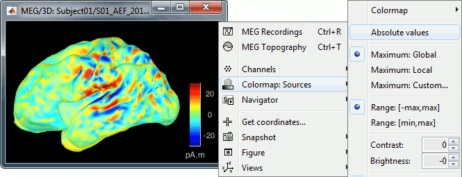
| Line 92: | Line 150: |
| This pattern is due to the '''orientation constraint''' imposed on the dipoles. On both sides of a sulcus, we have defined dipoles that are very close to each other, but with opposite orientations. If we observe a pattern of activity on one side of a suclus that can be assimilated to an electric dipole (green arrow), the minimum norm model will try to explain it with the dipoles that are available in the head model (red and blue arrows). Because of the dipoles orientations, it translates into positive values (red arrows) on one side of the sulcus and negative on the other side (blue arrows). | '''More on sign ambiguity: '''On opposite walls of a sulcus, brain source are very close to each other, with opposite orientations. If the true brain activity sits only on one side of a sulcus as shown below with a green arrow, the MN-imaging brain map lower spatial resolution will spread the estimated currents over multiple nearby locations, shown with the red and blue arrows below, which have opposite default directions that are imposed by anatomy (dipoles pointing outwards the cortical surface). The signs of the current flows will be opposite, with positive values (red arrows) on one side of the sulcus and negative values on the other side (blue arrows). |
| Line 96: | Line 154: |
| When displaying the cortical maps at one time point, we are usually not interested by the sign of the minimum norm values but rather by their amplitude. This is why we always display them by default with the colormap option "'''absolute values'''" selected. However, we cannot simply discard the sign of these values because we need them for other types of analysis, typically time-frequency decompositions and connectivity analysis. For estimating frequency measures on those source maps, we need to keep the oscillations around zero. == Source map normalization == The current density values returned by the minimum norm method have a few problems: * They depend a lot on the SNR of the signal, which may vary a lot between different subjects. * Their amplitude is therefore difficult to interpret directly. * The values tend to be always higher at the superficy of the brain (close to the sensors). * The maps are sometimes patchy and difficult to read. Normalizing the current density maps with respect with a baseline (noise recordings or resting state) can help with all these issues at the same time. Some normalizations can be computed independently from the recordings, and saved as part of the linear source model (dSPM, sLORETA, MNp). An other way of proceeding is to compute a Z-score baseline correction from the current density maps. All the normalizations options do not change your results, they are just different ways at looking at the same minimum norm maps. If you look at the time series associated with one source, it would be exactly the same for all the normalizations, except for a scaling factor. What changes is only the relative weights between the sources, and these weights do not change over time. ==== dSPM, sLORETA, MNp ==== * In Run#01, right-click on the average response for the '''deviant''' stim > '''Compute sources [2015]'''.<<BR>>Select sucessively the three normalization options: dSPM, sLORETA, MNp (constrained/normal). * SCREEN CAPTURES ==== Z-score ==== SCREEN CAPTURE ==== Typical recommendations ==== * Use non-normalized current density maps for: * Computing shared kernels applied to single trials. * Averaging across MEG runs. * Computing time-frequency decompositions or connectivity measures on the single trials. * Use normalized maps (dSPM, sLORETA, MNp, Z-score) for: * Calculating sources for average responses * Exploring visually the ERP/ERF at the source level, * Normalizing the subjects condition averages before a group analysis. * '''sLORETA, Kernel only, Unconstrained''' * Open solutions #3 (wMNE), #4 (dSPM) and #5 (sLORETA), all unconstrained. * Notice that the units are different: wMNE values are in pAm, dSPM and sLORETA are in arbitrary units (never try to compare these values to anything but the exact same type of inverse solution) * Observe around 46ms the respective behavior of these three solutions: * 3) wMNE tends to highlight the top of the gyri and the superficial sources, * 4) dSPM tends to correct that behavior and may give higher values in deeper areas, * 5) sLORETA produces a very smooth solution where all the potentially activated area of the brain (given to the low spatial resolution of the source localization with MEG/EEG) is shown as connected, regardless of the depth of the sources.<<BR>> Now delete all these files when you're done, and keep only the initial solution: wMNE, Constrained. == Computing sources for multiple data files == '''UNCONSTRAINED MN''' The sources file we are observing was computed as an ''inversion kernel''. It means that we can apply it to any similar recordings file (same subject, same run, same positions of sensors). But in our TutorialCTF database, the ''MN: MEG'' node only appears in the the ''ERF ''file, not in the ''Std ''one. What is it necessary to share an inversion kernel between different recordings ? 1. Compute another source estimation: but instead of clicking on the ''Compute sources'' from the ''ERF ''recordings popup menu (which would mean that you only want sources for this particular recordings file), get this menu from the ''Right''''' condition'''. This means that you want the inversion model to be applied to all the data in the condition. 1. Select "Minimum Norm Imaging", click on Run. 1. Three new nodes are available in the tree:<<BR>><<BR>> {{attachment:popupComputeMulti.gif}} {{attachment:treeMinNormMulti.gif}} 1. The actual inversion kernel you have just computed (1), contains the same information as the one from the previous section (Computing sources for a single data file). Note that you cannot do anything with this file: if you right-click on it, you can see that there are no ''Display ''menu for it. * Two links (2) that allow you apply this inversion kernel to the data files available in this condition (''ERF ''and ''Std''). In their popup menus, there are all the display options introduced in the previous section. * These links are not saved as files but as specific strings in the database: "link|kernel_file|data_file". This means that to represent them, one should load the shared kernel, load the recordings, and multiply them. * The sources for the ''Std ''file do not have any meaning, do not even try to open it. It was just to illustrate the way a kernel is shared 1. Double-click on both sources files available for ''Right / ERF'' (link and non-link), and verify at many different times that the cortical maps are exactly the same in both cases. 1. You can estimate the sources for many subjects or conditions at once, as it was explained for the head models in previous tutorial: the ''Compute sources'' menu is available on all the subjects and conditions popup menus. 1. Delete the shared kernel (1), we don't need redundant and confusing information for the next steps. Observe that both links disappear at the same time. == Average in source space == * Now we have the source maps available for all the trials, we average them in source space. * Select the folders for '''Run01 '''and '''Run02 '''and the ['''Process sources'''] button on the left. * Run process "'''Average > Average files'''": Select "'''By trial group (subject average)'''" . {{http://neuroimage.usc.edu/brainstorm/Tutorials/Auditory?action=AttachFile&do=get&target=process_average_results.gif|process_average_results.gif|height="376",width="425",class="attachment"}} * Double-click on the source averages to display them (standard=top, deviant=bottom). . {{http://neuroimage.usc.edu/brainstorm/Tutorials/Auditory?action=AttachFile&do=get&target=average_source.gif|average_source.gif|height="321",width="780",class="attachment"}} * Note that opening the source maps can be very long because of the online filters. Check in the Filter tab, you probably still have a '''100Hz low-pass filter''' applied for the visualization. In the case of averaged source maps, the 15000 source signals are filtered on the fly when you load a source file. This can take a significant amount of time. You may consider unchecking this option if the display is too slow on your computer. |
For visualization purposes, we are mostly interested at this stage in visualizing the magnitude of brain activity, hence the default colormap option "'''absolute values'''" being selected. == Unconstrained orientations == The "loose constraints" and "unconstrained" options for source orientations yield 3 time series per brain location (from three orthogonal elementary sources), which increases the dimensionality of the source maps, hence complexify their interpretation, but produces smoother renderings of current flows. We recommend these options when using an MRI template instead of the individual MRI volume of study participants, or when studying subcortical brain structures. Unconstrained maps can subsequently be [[https://neuroimage.usc.edu/brainstorm/Tutorials/PCA#Unconstrained_source_flattening_with_PCA|converted to "flat" maps]] with a single orientation per location. Here we will illustrate the fully unconstrained case. The procedure for the loose constraints options is similar. * In Run#01, right-click on the trial average of the '''deviant''' condition > '''Compute sources [2018]'''.<<BR>>Select the options: '''Minimum norm''' imaging, '''Current density''' map, '''Unconstrained'''. * Double-click on the source file produced (brain icon, labelled with "Unconstr") and on the corresponding sensor data file. The two brain maps below represent the same file at 91ms, with different colormap options (absolute values on the left, relative values on the right). Explanations below. <<BR>><<BR>> {{attachment:minnorm_unconstr_all.gif||height="413",width="652"}} * Again, using unconstrained/loose source orientations consists of '''triplets of dipoles with orthogonal orientations at each cortex location'''. To display their activity in a visually-meaningful manner, we first need to reduce the dimensions of the source data and color code the outcome. Brainstorm displays the '''norm of the vectorial sum of the three orientations at each vertex'''. <<BR>>S = sqrt(Sx^2^ + Sy^2^ + Sz^2^) <<BR>><<BR>> {{attachment:minnorm_unconstr_sketch.gif||height="158",width="476"}} * This explains that only '''positive values''' are displayed over the source map. Note that the actual full values along each orientation (x,y,z) are signed and can be retrieved from the source file for further derivations (e.g., spectral analyses). * The unconstrained/loose orientation maps are typically smoother than with the constrained orientation option (but see post-processing steps below) because they are less overly sensitive to changes in the curvature of the cortex. * You may delete the unconstrained source file: we will not use this option further in the introduction tutorials. Please refer to the tutorial [[http://neuroimage.usc.edu/brainstorm/Tutorials/Epilepsy|EEG and epilepsy]] for further exploration of this option. == Standardization of source maps == Standardization procedures can compensate some of the bias of MN imaging source maps towards superficial source locations (in both MEG and EEG) and radially oriented current flows (in MEG). It also enables a fairer comparison of brain activity between individuals, based on its relative change with a data segment of reference. Reference data segments can be extracted from empty-room recordings (MEG), pre-stimulus baseline or resting state data (MEG and EEG). dSPM and sLORETA proceed to such standardization within their respective source mapping procedures. Brainstorm also features a Z-score normalization process, which enables a versatile definition of the reference data segment. Source map standardization does not alter the dynamics of the source time series and only scales their respective amplitude changes. The scaling factors are different at each brain location, hence the resulting source maps will look different than the original MN images, but with the same temporal dynamics. ==== dSPM, sLORETA (embedded standardization) ==== * In Run#01, right-click on the average sensor data of the '''deviant''' condition > '''Compute sources [2018]'''.<<BR>>Select successively the two normalization options: dSPM, sLORETA, ('''constrained''').<<BR>><<BR>> {{attachment:minnorm_normfiles.gif}} * Double-click on all the resulting source files to compare them (screen capture below is at the '''143-ms''' time point): <<BR>><<BR>> {{attachment:minnorm_normalized.gif||height="156",width="628"}} * '''Current density maps (MN imaging)''': without further standardization, MN imaging tends be biased towards the most superficial gyral crowns (see Z-score procedure below). * '''dSPM''': compensates some of this bias. The amplitude of brain maps are converted to z-scores. You may adjust the z-scores with the number of trials used to obtain the sample average via specific process "Sources > '''Scale averaged dSPM'''" (see [[https://neuroimage.usc.edu/brainstorm/Tutorials/SourceEstimation#Averaging_normalized_values|Averaging normalized values]]). * '''sLORETA''': also produces unitless maps, but the statistics are proper to the method and therefore, are not related to z-scores. ==== Z-score transformation of brain maps ==== * The '''Z-transformation''' of MN imaging brain maps centre source amplitudes around their mean over a reference segment, and scale them with respect to their standard deviation over the same reference segment: '''Z = (Data - <<HTML(μ)>>) / <<HTML(σ)>>''' * The mean and standard deviation parameters are estimated from the data and are specific of each source location. Hence, sources with lower fluctuations over the reference segment (e.g., with less noise, or overall smaller amplitude) will be boosted by the transformation. * In Process1: Select the constrained current density map (file ''MN: MEG(Constr)''). * Run process "'''Standardize > Baseline normalization'''", '''[-100,-1.7]ms''', '''Z-score transformation''' <<BR>>Do not select "Use absolute values" as for now, we wish to preserve the sign of source amplitudes.<<BR>><<BR>> {{attachment:zscore_process.gif||height="530",width="558"}} * Double-click on the new brain map file (with the "| zscore" tag). <<BR>><<BR>> {{attachment:zscore_cortex.gif||height="153",width="657"}} * We can appreciate that the standardized map is now qualitatively similar to dSPM and sLORETA versions. * A map value of 3 means that the source amplitude at this time point is 3 times above the typical amplitude of that same source during the reference segment. * Please note Brainstorm's online filters __do not__ affect the z-transformed source maps. Using the Filter tab and applying a bandpass filter will update the display all sensor time series and source maps on display, except the z-transormed maps. * If you wish to use a reference segment from another data file (e.g., a resting state recording as reference for the current task recording), use the '''Process2 '''process tab''' '''by dragging and dropping the reference source map in the Files A list on the left, and the source maps to be standardized in the Files B list on the right. ==== Recommended options ==== * Use non-standardized '''current density maps (MN imaging)''' for: * Computing imaging kernels shared across single trials. * Averaging files across several MEG/EEG runs. * Deriving spectral, time-frequency decompositions, phase-amplitude, or connectivity measures on single trials. * Use '''standardized maps''' (dSPM, sLORETA, Z-score) for: * Producing source maps of trial averages (ERP/ERF). * Before running a group analysis of source maps. * Recommended standardization approach: * dSPM and sLORETA are convenient linear measures which are easy to manipulate with Brainstorm. * sLORETA maps are spatially smoother but with no direct statistical interpretation without further inference testing. * dSPM and Z-score maps are statistically interpretable as excursions with respect to a reference data segment (Z-score), or with respect to noise covariance statistics (dSPM). == Delete your experiments == Before we proceed with the rest of the tutorial, please delete the source maps computed so far. * Select all the source files you computed until now and '''delete''' them. <<BR>><<BR>> {{attachment:delete_norm.gif||height="172",width="474"}} == Computing sources for single trials == MN imaging models are linear: their respective imaging kernels can be pre-computed from anatomy and sensor locations only, then can be applied at once on long, ongoing or several epoched data segments on the fly. Here we show how to obtain source maps across multiple single trial epochs. * Right-click on the '''head model''' or the '''folder '''for Run#01 > '''Compute sources [2018]'''.<<BR>>Select: '''Minimum norm''' imaging, '''Current density''' map, '''Constrained''': Normal to cortex<<BR>><<BR>> {{attachment:minnorm_shared_popup.gif||height="273",width="500"}} * This procedure produces a '''shared imaging kernel''' (white brain icon) that is comon to all data files in Run #01. If you right-click on this new file, a warning message pops up that says "Inversion kernel". This file does not contain source maps, only the linear operator (kernel) to convert the sensor data into source maps. <<BR>><<BR>> {{attachment:minnorm_shared_kernel.gif}} * All data files in Run #01 (averages and single epochs) now show a '''link to a''' '''source file''' (grey brain icon), which is a virtual brain map that is computed on the fly when visualized: Brainstorm multiplies the imaging kernel by the sensor data time series, for greater computational and data storage efficacy. You may now visualize and manipulate these virtual source maps just like the maps we computed above.<<BR>><<BR>> {{attachment:minnorm_links.gif||height="176",width="513"}} == Averaging in source space == ==== Computing the average ==== * First compute the same source model for the the second acquisition run.<<BR>>In Run#02, right-click on the '''head model''' or the '''folder '''> '''Compute sources [2018]'''.<<BR>>Select: '''Minimum norm''' imaging, '''Current density''' map, '''Constrained''': Normal to cortex<<BR>><<BR>> {{attachment:minnorm_run02.gif||height="242",width="245"}} * Now we have the source maps available for all the recordings, we can '''average them in source space''' across runs. This allows us to average MEG recordings that were recorded with different head positions (in this case Run#01 and Run#02 have different channel files so they could potentially have different head positions preventing the direct averaging at the sensor level). * Thanks to the linearity of the minimum norm model: MN(Average(trials)) = Average(MN(trials))<<BR>>The two following approaches are equivalent: 1. Averaging the sources of all the individual trials across runs, 1. Averaging the sources for the sensor averages that we already computed for each run. * We will use the second option: using the sources for the sensor-level averages. It is a lot faster because it needs to read 4 files (one average file per run and per condition) instead of 456 files (total number of good trials in the two runs). * Drag and drop to the Process1 tab the average recordings for '''Run01 '''and '''Run02''', then press the ['''Process sources'''] button on the left to select the source files instead of the MEG recordings. * Run process "'''Average > Average files'''": <<BR>>Select "'''By trial group (subject average)'''" to average together files with similar names. <<BR>>Select "'''Arithmetic average'''" function. <<BR>>Check "'''Weighted average'''" to account for the different numbers of trials in both runs.<<BR>><<BR>> {{attachment:average_process.gif||height="565",width="526"}} * The two averages that are produced (one for each condition) are saved in the folder '''Intra-subject'''. This is where all the files computed using information from multiple folders within the same subject are saved. If you prefer to have them somewhere else, you can create new folders and move them there, just like you would do with a regular file explorer. <<BR>><<BR>> {{attachment:average_files.gif||height="159",width="268"}} * The file comments say "2 files" because they were computed from two averages each (one from each run), but the number of corresponding trials is correctly updated in the file structure. <<BR>>Right-click on each of them > File > View file contents, and check the '''Leff''' field: <<BR>>78 trials for the deviant condition, 378 trials for the standard condition. * Double-click on the source averages to display them (deviant=top, standard=bottom). <<BR>>Open the sensor-level averages as a time reference. <<BR>>Use the predefined view "Left, Right" for looking at the two sides at the same time (shortcut: "7").<<BR>><<BR>> {{attachment:average_display_mn.gif||height="296",width="530"}} ==== Visualization filters ==== * Note that opening the source maps can be very long because of the filters for visualization. Check in the '''Filter''' '''tab''', you may have a''' '''filter applied with the option "'''Filter all results'''" selected. In the case of averaged source maps, the 15,000 source signals are filtered on the fly when you load a source file. This filtering of the full source files can take a significant amount of time, consider unchecking this option if the display is too slow on your computer. <<BR>><<BR>> {{attachment:filter_sources.gif||height="163",width="207"}} * It was not a problem until now because the source files were saved in the compact form (Kernel*recordings) and the visualization filters were applied on the recordings, then projected to the source space. This fast option is not available anymore with these averages across runs. * The visualization filters will not be available anymore after we apply a Z-score normalization. If we want to display Z-score source maps that are smoothed in time, we will have to apply explicitly the filters on the file, with the Process1 tab. ==== Low-pass filter ==== * Clear the Process1 list, then drag and drop the new averages in it. * Run process "'''Pre-process > Band-pass filter'''": [0,40] Hz<<BR>><<BR>> {{attachment:average_filter.gif||height="338",width="476"}} * '''Epochs are too short''': Look at the filter response, the expected transient duration is at least 78ms. The first and last 78ms of the average should be discarded after filtering. However, doing this would get rid of almost all the 100ms baseline, which we need for normalization. As mentioned [[http://neuroimage.usc.edu/brainstorm/Tutorials/Epoching#Epoch_length|here]], we should have been importing longer epochs in order to filter and normalize the averages properly. <<BR>><<BR>> {{attachment:average_filter2.gif||height="323",width="378"}} ==== Z-score normalization ==== * In Process1, select the two filtered averages. * Run process "'''Standardize > Baseline normalization'''", baseline='''[-100,-1.7]ms, ''''''Z-score.'''<<BR>><<BR>> {{attachment:average_zscore.gif||height="292",width="539"}} * Four new files are accessible in the database: two filtered and two filtered+normalized. <<BR>><<BR>> {{attachment:average_zscore_files.gif||height="205",width="341"}} * Double-click on the source averages to display them (deviant=top, standard=bottom).<<BR>><<BR>> {{attachment:average_display_zscore.gif||height="295",width="530"}} * The Z-score source values at 90ms are higher for the standard condition (~25) than for the deviant condition (~15). We observe this because the two conditions have very different signal-to-noise ratios. The standard condition has about 5x more trials, therefore the standard deviation over the baseline is a lot lower, leading to higher Z-score. * '''Delete''' the non-normalized filtered files, we will not use them in the following tutorials. <<BR>><<BR>> {{attachment:average_zscore_files2.gif||height="147",width="294"}} == Note for beginners == Everything below is advanced documentation, you can skip it for now. <<EmbedContent("http://neuroimage.usc.edu/bst/get_prevnext.php?skip=Tutorials/Scouts")>> |
| Line 173: | Line 271: |
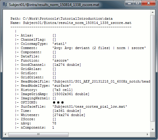
| == Averaging normalized values == Averaging normalized source maps within a single subject requires more attention than averaging current density maps. Since averaging reduces variance, the resulting source maps will have a different statistical distribution than the nominal distribution of the individual maps. For example, averaging z-score normalized maps will result in maps with variance less than 1. The same holds true for dSPM maps. Assuming independent samples, the variance of an average of N maps drops by 1/N. For this reason, it is generally recommended to select the "Weighted average" option in the ‘Average files’ process when averaging trials or source maps (which performs mean(x) = (N1*sum(x1(i)) + N2*sum(x2(i)) + …)/ (N1+N2+…) ) in order to keep track of the number of samples and the actual variance of averaged statistical maps. '''dSPM''' * An averaged dSPM map has variance equal to 1/N (and thus standard deviation equal to 1/sqrt(N)). Therefore one could multiply the averaged dSPM map by sqrt(N) in order to maintain variance 1 under the null hypothesis. In previous versions of Brainstorm, this was done automatically when visualizing the files, and when averaging source maps with the option "Adjust normalized source maps for SNR increase". To simplify the interface and make the interpretation of maps more intuitive and consistent with other cases (min-norm, z-scored), we now dropped this option. Thus averaging dSPM maps now results in maps with variance less than 1, and is consistent with handling min-norm, z-scored and sLORETA maps. * Ajusting an averaged dSPM file by this sqrt(N) factor is still possible manually, eg. in order to visualize cortical maps that can be interpreted as Z values. Select the average dSPM files in Process1 and run process "Sources > '''Scale averaged dSPM'''". This should be used only for visualization and interpretation, scaled dSPM should never be averaged or used for any other statistical analysis. <<BR>><<BR>> {{attachment:dspm_scale.gif||height="307",width="547"}} '''Z-score''' * The same SNR issues arise while averaging Z-scores: the average of the Z-scores is lower than the Z-score of the average. * When computing averages at the subject level: Always '''avoid averaging Z-score maps'''. <<BR>>Average the current density maps, then normalize. '''sLORETA''' * This normalization is not based on the SNR of signal, but rather on the spatial smoothness of the maps. Managing these maps is similar to min-norm maps: the variance of the individual maps is not explicitly modeled or known analytically. * As in other cases, sLORETA(Average(trials)) = Average(sLORETA(trials)), and this relationship is guaranteed to hold with averaging uneven number of samples when using the option "Weighted average". <<TAG(Advanced)>> |
|
| Line 174: | Line 295: |
| * '''Standard:''' (Right-click on the 3D figures > Snapshot > Time contact sheet) . Explain qhat to do to make nice contact sheets this way * '''Deviant:''' . {{http://neuroimage.usc.edu/brainstorm/Tutorials/Auditory?action=AttachFile&do=get&target=average_source_deviant_left.gif|average_source_deviant_left.gif|height="263",width="486",class="attachment"}} * Contact sheets: in time or in space, for each orientation. You can try all the menus. Example: Right-click on the figure > Snapshot > Volume contact sheet: axial: <<BR>><<BR>> {{attachment:popupSnapshot.gif}} {{attachment:contactAxial.gif||height="288px",width="322px"}} * '''Movies''': Right-click on any figure > Snapshot > '''Movie (time): All figures''' (click to download video) [[http://neuroimage.usc.edu/wikidocs/average_sources.avi|{{http://neuroimage.usc.edu/brainstorm/Tutorials/Auditory?action=AttachFile&do=get&target=average_source_video.gif|http://neuroimage.usc.edu/brainstorm/wikidocs/average_sources.avi|height="258",width="484",class="attachment"}}]] |
A good way to represent what is happening in time is to generate contact sheets or videos. Right-click on any figure and go to the menu Snapshot to check out all the possible options. For a nicer result, take some time to adjust the size of the figure, the amplitude threshold and the colormap options (hiding the colorbar can be a good option for contact sheets). A time stamp is added to the captured figure. The size of the text font is fixed, so if you want it to be readable in the contact sheet, you should make you figure very small before starting the capture. The screen captures below where produced with the colormap "hot". * '''Contact sheet:''' Right-click on any figure > Snapshot > '''Time contact sheet: Figure'''<<BR>><<BR>> {{attachment:contact_options.gif||height="209",width="128"}} {{attachment:contact_image.gif||height="249",width="405"}} * '''Movies''': Right-click on any figure > Snapshot > '''Movie (time): All figures'''<<BR>><<BR>> {{attachment:video_options.gif||height="263",width="126"}} [[http://neuroimage.usc.edu/wikidocs/average_sources_unconstr.avi|{{attachment:video_vlc.gif|http://neuroimage.usc.edu/wikidocs/average_sources_unconstr.avi|height="262",width="409"}}]] |
| Line 183: | Line 304: |
| == Advanced options == Let's introduce briefly the other options offered for the source estimation. Right-click again on Right / ERF > Compute sources. Click on "Expert mode", you see more options appearing in the window. If you click on Run, you have access to all the options of the wMNE algorithm. {{attachment:panelExpert.gif}} {{attachment:panelOptions.gif}} === Beamformer options === === Dipole fitting options === |
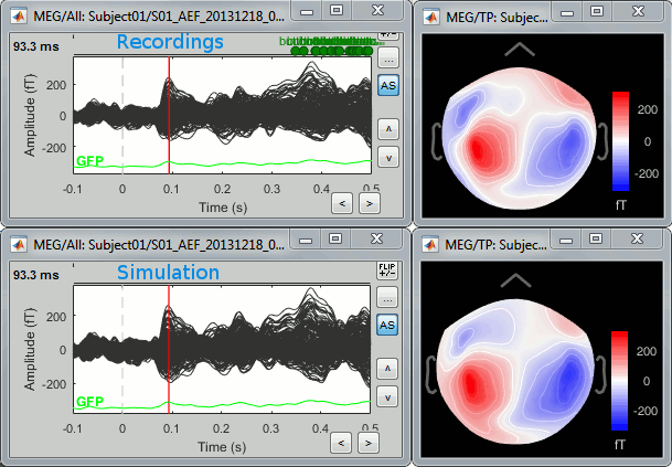
== Model evaluation == One way to evaluate the accuracy of the source reconstruction if to simulate recordings using the estimated source maps. This is done simply by multiplying the source time series with the forward model:<<BR>>MEG_simulated [Nmeg x Ntime] = Forward_model [Nmeg x Nsources] * MN_sources [Nsources x Ntime]<<BR>>Then you can compare visually the original MEG recordings with the simulated ones. More formally, you can compute an error measure from the residuals (recordings - simulated). To simulate MEG recordings from a minimum norm source model, right-click on the source file, then select the menu "'''Model evaluation > Simulate recordings'''". . {{attachment:model_popup.gif||height="151",width="597"}} Open side-by-side the original and simulated MEG recordings for the same condition: . {{attachment:model_results.gif||height="218",width="332"}} <<TAG(Advanced)>> == Advanced options: Minimum norm == Right-click on the '''deviant average''' for '''Run#01''' > '''Compute sources [2018]'''. <<BR>>Click on the button ['''Show details'''] to bring up all the advanced minimum norm options. <<HTML(<div style="padding: 0px 0px 0px 10px; float: right;">)>> {{attachment:minnorm_details.gif||height="392",width="390"}} <<HTML(</A></div>)>> === Depth weighting === Briefly, the use of various depth weightings was far more debated in the 1990s, before the introduction of MNE normalization via dSPM, sLORETA, and other "z-scoring" methods, which mostly cancel the effects of depth weighting (put another way, after normalization min norm results tend to look quite similar whether depth weighting is used or not). By modifying the source covariance model at each point in the source grid, deeper sources are "boosted" to increase their signal strength relative to the shallower dipoles; otherwise, the resulting MNE current density maps are too dominated by the shallower sources. If using dSPM or sLORETA, little difference in using depth weighting should be noted. To understand how to set these parameters, please refer to the [[https://mne.tools/mne-c-manual/MNE-manual-2.7.3.pdf|MNE manual]]. (options --depth, --weightexp and --weightlimit). === Noise covariance regularization [TODO] === MNE and dipole modeling are best done with an accurate model of the noise covariance, which is generally computed from experimental data. As such, these estimates are themselves prone to errors that arise from relatively too few data points, weak sensors, and strange data dependencies that can cause the eigenspectrum of the covariance matrix to be illconditioned (i.e. a large eigenvalue spread or matrix condition number). In Brainstorm, we provide several means to "stabilize" or "regularize" the noise covariance matrix, so that source estimation calculations are more robust to small errors. * '''Regularize noise covariance''': The L2 matrix norm is defined as the largest eigenvalue of its eigenspectrum. This option adds to the covariance matrix a diagonal matrix whos entries are a fraction of the matrix norm. The default is 0.1, such that covariance matrix is stabilized by adding to it an identity matrix that is scaled to 10% of the largest eigenvalue. * '''Median eigenvalue''': The eigenspectrum of MEG data can often span many decades, due to highly colored spatial noise, but this broad spectrum is generally confined to the first several modes only. Thus the L2 norm is many times greater than the majority of the eigenvalues, and it is difficult to prescribe a conventional regularization parameter. Instability in the inverse is dominated by defects found in the smallest eigenvalues. This approach stabilizes the eigenspectrum by replicating the median (middle) eigenvalue for the remainder of the small eigenvalues. * '''Diagonal noise covariance''': Deficiencies in the eigenspectrum often arise from numerical inter-dependencies found among the channels, particularly in covariance matrices computed from relatively short sequences of data. One common method of stabilization is to simply take the diagonal of the covariance matrix and zero-out the cross-covariances. Each channel is therefore modeled as independent of the other channels. The eigenspectrum is now simply the (sorted) diagonal values. * '''No covariance regularization''': We simply use the noise covariance matrix as computed or provided by the user. * '''Automatic shrinkage''': Stabilization method of Ledoit and Wolf (2004), still under testing in the Brainstorm environment. Basically tries to estimate a good tradeoff between no regularization and diagonal regularization, using a "shrinkage" factor. See Brainstorm code "bst_inverse_linear_2018.m" for notes and details. * '''Recommended option''': This author (Mosher) votes for the '''median eigenvalue '''as being generally effective. The other options are useful for comparing with other software packages that generally employ similar regularization methods. '''[TODO]''' === Regularization parameter [TODO] === In minimum norm estimates, as mentioned above in the comparisons among methods, the data covariance matrix is essentially synthesized by adding the noise covariance matrix to a modeled signal covariance matrix. The signal covariance matrix is generated by passing the source prior through the forward model. The source prior is in turn prescribed by the source model orientation and the depth weighting. A final regularization parameter, however, determines how much weight the signal model should be given relative to the noise model, i.e. the "signal to noise ratio" (SNR). In Brainstorm, we follow the definition of SNR as first defined in the original MNE software of Hamalainen. The signal covariance matrix is "whitened" by the noise covariance matrix, such that the whitened eigenspectrum has elements in terms of SNR (power). We find the mean of this spectrum, then take the square root to yield the average SNR (amplitude). The default in MNE and in Brainstorm is "3", i.e. the average SNR (power) is 9. * '''Signal-to-noise ratio''': Use SNR of 3 as the classic recommendation, as discussed above. * '''RMS source amplitude''': An alternative definition of SNR, but still under test and may be dropped. '''[TODO]''' |
| Line 191: | Line 346: |
| * '''Full results''': Saves in one big matrix the values of all the sources (15000) for all the time samples (375). The size in memory of such a matrix is about 45Mb for 300ms of recordings. This is still reasonable, so you may use this option in this case. But if you need to process longer recordings, you may have some "Out of memory" errors in Matlab, or fill your hard drive quickly. * '''Kernel only''': Saves only the ''Inversion kernel'', a matrix that describes how to compute the sources when you know the values at the sensor level. So its size is: number of sources (15000) x number of sensors (151). This is possible because these minimum norm methods are linear methods. * To get the sources time series, you just need to multiply this kernel by the MEG recordings. * '''Full results '''=''' Inversion kernel '''*''' Recordings''' * The size of this matrix is about 18Mb. In this case, the difference is not very important because we only process 375 time samples. But this inversion kernel is independent from the recordings length, so you can easily scale its computation to much longer recordings. * '''Default ?''' * Probably "''Kernel only''", as it is faster and produces smaller files. * All the following operations in Brainstorm will be exactly the same either way. Each time you access the sources values, the program has to do the multiplication Kernel * Recordings, but this is done in a totally transparent way. * The only reason that would make you choose the "''Full results''" options would be any interest in having the full matrix in one file, in case you want to process the sources values by yourself (filtering, statistics, display...). === Signal properties === * '''Signal to noise ratio (SNR)''': An estimate of the amplitude SNR of the recordings, as defined in MNE (--snr option in MNE), used to compute the regularization parameter (lambda^2 = 1/SNR^2). The default value is SNR = 3. Automatic selection of the regularization parameter is currently not supported. * '''PCA Whitening''': Parameter introduced by Rey Ramirez. For more information, see the code of bst_wmne function. === Noise covariance matrix === * '''Full noise covariance''': Use the full noise covariance matrix available in Brainstorm database. If the noise covariance file previously computed in is a diagonal matrix (as it is the case in this tutorial), this value is ignored, and the "diagonal noise covariance" option is used instead. * '''Diagonal noise covariance''': Discard the off-diagonal elements of the noise covariance matrix (assuming heteroscedastic uncorrelated noise). Corresponds in MNE to the --diagnoise option. * '''Regularize noise covariance''': Regularize the noise-covariance matrix by the given amount for each type of sensor individually (value is restricted to the range 0...1). For more information, please refer to the MNE manual, section 6.2.4 (options --magreg, --gradreg and --eegreg). === Depth weighting === The minimum-norm estimates have a bias towards superficial currents. This tendency can be alleviated by adjusting these parameters. To understand how to set these parameters, please refer to the MNE manual (options --depth, --weightexp and --weightlimit). |
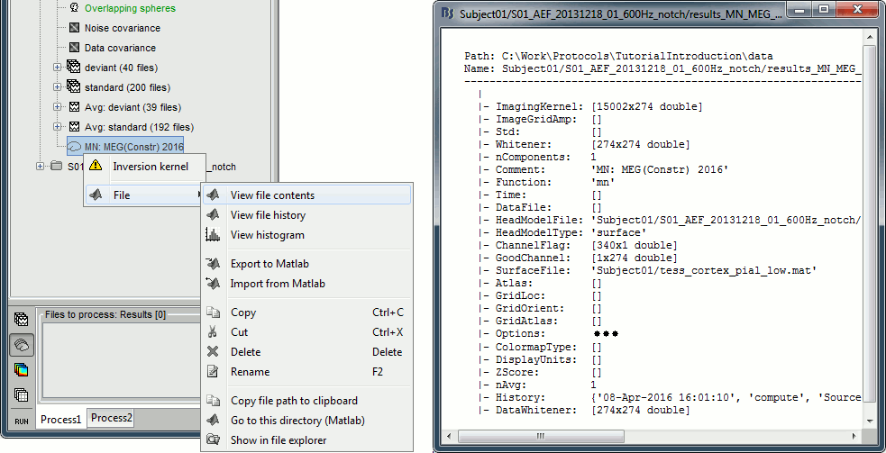
As mentioned above, these methods create a convenient linear imaging kernel that is "tall" in the number of elemental dipoles (one or three per grid point) and "wide" only in the number of sensors. At subsequent visualization time, we efficiently multiply the kernel with the data matrix to compute the min norm images. For some custom purposes, however, a user may find it convenient to pre-multiply the data matrix and generate the full source estimation matrix. This would only be recommended in small data sets, since the full results can become quite large. * '''Kernel only''': Saves only the linear inverse operator, a model that converts sensor values into source values. The size of this matrix is: number of sources (15000) x number of MEG sensors (274). The multiplication with the recordings is done on the fly by Brainstorm in a transparent way. For long recordings or numerous epochs, this form of compact storage helps saving a lot of disk space and computation time, and it speeds up significantly the display. Always select this option when possible. * '''Full results''': Saves in one big matrix the values of all the sources (15,000) for all the time samples (361). The size in memory of such a matrix is about 45Mb for 600ms of recordings. This is still reasonable, so you may use this option in this case. But if you need to process longer recordings, you may face "Out of memory" errors in Matlab, or fill your hard drive quickly. * Full results [15000x361] = Inverse kernel [15000x274] * Recordings [274x361] == Advanced options: LCMV beamformer == As mentioned in the introduction above, two other methods can be selected for source estimation, a beamformer and dipole modeling. In this section, we review the options for the beamformer. On top of the noise covariance matrix, you need to estimate a [[http://neuroimage.usc.edu/brainstorm/Tutorials/NoiseCovariance#Data_covariance|data covariance matrix]] in order to enable the option "LCMV beamformer" in the interface. Note that pre-whitening with the noise covariance matrix has not yet been implemented for the LCMV beamformer, and only the [[Tutorials/NoiseCovariance#Data_covariance|data covariance]] is used in the current version. The noise covariance has no impact on the LCMV beamformer results. However, if there is no noise covariance file available in the database, the "Compute sources" interface returns an error: to go around this limitation, you may select the "No noise modeling (identity matrix)" option in the contextual menu for the noise covariance. <<HTML(<div style="padding: 0px 0px 0px 10px; float: right;">)>> {{attachment:lcmv_options.gif||height="350",width="390"}} <<HTML(</A></div>)>> '''Measure''' The only option "Pseudo Neural Activity Index" (PNAI), is named after the definition of the Neural Activity Index (NAI). We have modified Van Veen’s definition to rely strictly on the data covariance, without need for a separate noise covariance matrix, but the basic premise is the same as in dSPM, sLORETA, and other normalizations. Viewing the resulting "map," in an identical manner to that with MNE, dSPM, and sLORETA described above, reveals possibly multiple sources as peaks in the map. Note that PNAI scores are unitless, because they correspond to standardized statistical fluctuations of neural currents. In this way, PNAI scores are analogous to z-scoring. '''Dipole orientations''' We recommend you choose "'''unconstrained'''" and let the later [[Tutorials/TutDipScan|Dipole scanning]] process, which finds the best fitting dipole at each time point, optimize the orientation with respect to the data. '''Data covariance regularization''' Same definitions as in MNE, only applied to the data covariance matrix, rather than the noise covariance matrix. Our recommendation is to use '''median eigenvalue'''. == Advanced options: Dipole modeling == Dipole modeling fits a single dipole at each potential source location to produce a dipole scanning map. This map can be viewed as a indication of how well, and where, the dipole fits at each time point. However, we recommend using the subsequent best-dipole fitting routine ([[Tutorials/TutDipScan|dipole scanning]]) to determine the final location and orientation of the dipole (one per time point). Please note that '''this function does not fit multiple simultaneous dipoles'''. Although not widely recognized, dipole modeling and beamforming are more alike than they are different – when comparing the inverse operators required to compute the dipole scanning map (dipole modeling) and the beamformer output map (LCMV), we see that they differ only in that the former uses an inverse noise covariance matrix while the latter replaces this with the inverse of the data covariance. <<HTML(<div style="padding: 0px 0px 0px 10px; float: right;">)>> {{attachment:dipoles_options.gif||height="314",width="390"}} <<HTML(</A></div>)>> '''Measure''' This field is now missing, but the resulting imaging kernel file is directly analogous to the PNAI result from LCMV beamforming. The user can display this scanning measure just as with the LCMV case, where again the normalization and units are a form of z-scoring. '''Dipole orientations''' Use "unconstrained source" modeling and let the process "[[Tutorials/TutDipScan|dipole scanning]]" optimize the orientation of the dipole for every time instance. '''Noise covariance regularization''' Similarly, use "median eigenvalue". <<HTML(<div style="clear: right;"></div>)>> The tutorial "[[http://neuroimage.usc.edu/brainstorm/Tutorials/PhantomElekta#Dipole_source_estimation|MEG current phantom (Elekta)]]" demonstrates dipole modeling of 32 individual dipoles under realistic experimental noise conditions. |
| Line 215: | Line 400: |
| == Equations == TODO: John |
== Combining MEG+EEG for source estimation == Magnetoencephalography and EEG sensor data can be processed jointly to produce combined source estimates. Joint processing presents unique challenges because EEG and MEG use head models that exhibit differing sensitivities to modeling errors, which can in turn lead to inconsistencies between EEG and MEG with respect to the (common) source model. In practice joint processing is relatively rare ([[https://www.frontiersin.org/articles/10.3389/fnins.2019.00076/full#B4|Baillet et al., 1999]]). However, these data are complementary, which means that joint processing can potentially yield insights that cannot be seen with either modality alone. For example, in the evoked responses in the data set used here, the first peak over the occipital areas is observed in MEG (90 ms) slightly before EEG (110 ms). This delay is too large to be caused by acquisition imprecisions. This indicates that we are not capturing the same brain processes with the two modalities, possibly because the orientation and type of activity in the underlying cortical sources is different. MEG and EEG have different sensitivities to source orientation and depth. Given the challenges of joint processing, our advice is to first look at the source reconstructions for the two modalities separately before trying to use any type of fusion technique. |
| Line 220: | Line 409: |
| == Rey on sLORETA == Yes in sLORETA the noise covariance is not used at all for the standardization process. It can be used modeling correlated noise and whitening, but that is optional. I have noticed that a lot of folks are confused about this and I have seen many statements in papers spreading this awful confusion. The sLORETA is standardized by the resolution matrix (diagonal for dipole orientations constraints, or block diagonals for free orientations). That is why sLORETA has zero localization bias for ALL point-spread functions, and why I always prefer sLORETA over dSPM, MNE, or any beamformer. This is all in the math .... but ..... just so that you know Fas Hsuan Lin's paper comparing sLORETA with dSPM, and MNE has a big mistake, the assumed source covariance matrix is not the identity matrix, and that violates the beauty of the math and results in non-zero localization bias. That's why in Brainstorm the prior source covariance matrix used for sLORETA automatically uses no depth bias compensation (identity matrix). sLORETA accomplishes depth bias compensation via the resolution matrix, NOT via the prior source covariance matrix. Trying to use a depth exponent of 0.7 or 0.8 like we do for MNE and dSPM will mess up sLORETA.You will not find this in a paper, but I checked it all out many years ago. This is critical. '''Explain sLORETA units (see email exchanges from Feb 2015) ''' <<TAG(Advanced)>> == Issues with dSPM average == Average(dSPM) is NOT equal to dSPM(Average). {{{ There is no problem for the MNE and sLORETA solutions, because the scaling of the noise covariance matrix doesn't impact the results. wMNE(Data, NoiseCov) = wMNE(Data, NoiseCov / N) So when we average we get: Average(wMNE(Trials, NoiseCov)) = wMNE(Average, NoiseCov) = wMNE(Average, NoiseCov / N) But for dSPM we have: dSPM(Data, NoiseCov) = dSPM(Data, NoiseCov / N) ./ sqrt(N) So when we average we get: Average(dSPM(Trials, NoiseCov)) = dSPM(Average, NoiseCov) = dSPM(Average, NoiseCov / N) ./ sqrt(N) }}} Rey: "Basically, the dSPM value at each location is equal to the wMNE value divided by the projection of the estimated noise covariance matrix onto each source point. After whitening, the operational noise covariance matrix is by definition the identity matrix, and hence the projection of the noise is equal to the L2 norm of the row vector of the wMNE inverse operator (in the case of fixed dipole orientations). So, dSPM is what you get when the rows of the wMNE inverse operator all have unit norm (i.e., they all point in different directions but lie in a unit hyper-sphere)." Rey: "dSPM is really a source mapping of SNR, not of activity. Hence, it's not all so surprising that the single trial SNR maps are smaller... "Rey: "Perhaps, dSPM should be used only for averaged data (i.e., ERF, ERP), at least until it's all figure out. In a way, dSPM is just MNE followed by the noise normalization. Thus, you could do all the single trial processing with the MNE algorithm, and only do the noise normalization when needed (e.g., after averaging or on single trials only if they are not going to be averaged)." |
|
| Line 252: | Line 410: |
| Document file tags Document file structure Differences for kernel vs. sources Differences for constrained vs. unconstrained in_bst_results to get the full sources or apply any process * You can have a look to the corresponding matrix file (right-click > File > View file contents). You would find all the options of forward and inverse modeling, and only one interesting field : '''ImagingKernel''', which contains the inversion kernel. It is a [nVertices x nChannels] matrix that has to be multiplied with the recordings matrix in order to get the activity for each source at all the time samples. * The minimum norm solution being a linear operation (the time series for each source is a linear combination of all the time series recorded by the sensors), we make this economy of saving only this linear operator instead of the full source matrix (nVertices x nTime) == References == * Dale AM, Liu AK, Fischl BR, Buckner RL, Belliveau JW, Lewine JD, Halgren E<<BR>>[[http://www.ncbi.nlm.nih.gov/pubmed/10798392|Dynamic statistical parametric mapping: combining fMRI and MEG for high-resolution imaging of cortical activity]]. Neuron 2000 Apr, 26(1):55-67 * Pascual-Marqui RD, [[http://www.ncbi.nlm.nih.gov/pubmed/12575463|Standardized low-resolution brain electromagnetic tomography (sLORETA): technical details]], Methods Find Exp Clin Pharmacol 2002, 24 Suppl D:5-12 == Additional discussions on the forum == |
==== Constrained shared kernel ==== Right-click on a shared inverse file in the database explorer > File > '''View file contents'''. . {{attachment:kernel_contents.gif||height="342",width="669"}} ==== Structure of the source files: results_*.mat ==== Mandatory fields: * '''ImagingKernel''': Linear inverse operator that must be multiplied by the recordings in order to get the full source time series. If defined, ImageGridAmp must be empty. . Size for constrained sources [Nsources x Nchannels] . Size for unconstrained sources [3xNsources x Nchannels]. Order of sources: source1.x, source1.y, source1.z, ... sourceN.z) * '''ImageGridAmp''': Full source time series, in Amper.meter. If this field is defined, ImagingKernel must be empty. If you want this field to be set instead of ImagingKernel, make sure you select the advanced option ''Full results'' when estimating the sources. . Size for constrained sources [Nsources x Ntime] . Size for unconstrained sources [3xNsources x Ntime]. Order of sources: source1.x, source1.y, source1.z, ... sourceN.z) * '''Time''': [1 x Ntime] Time values for each sample recorded in F, in seconds. * '''nComponents''': Number of dipoles per grid point: 1=Constrained, 3=Unconstrained, 0=Mixed. In the case of mixed head models, the atlas GridAtlas documents region by region how the list of grid points matches the list of dipoles. * '''Function''': Type of values currently saved in the file: 'mn', 'mnp', 'dspm', 'dspm2018', 'dspm2018sc', 'sloreta', 'lcmv', 'lcmvp', 'lcmvnai', 'lcmvpow', 'gls', 'glsp', 'glsfit', 'glschi', 'zscore', 'ersd'... * '''HeadModelType''': Type of source space used for this head model ('surface', 'volume', 'mixed'). * '''HeadModelFile''': Relative path to the head model used to compute the sources. * '''SurfaceFile''': Relative path to the cortex surface file related with this head model. * '''Atlas''': Used only by the process "Sources > Downsample to atlas". * '''GridLoc''': [Nvertices x 3], (x,y,z) positions of the grid of source points. In the case of a surface head model, it is empty and you read directly the positions from the surface file. * '''GridOrient''': [Nvertices x 3], direction of the normal to the surface for each vertex point (copy of the 'VertNormals' matrix of the cortex surface). Empty in the case of a volume head model or unconstrained sources. * '''GridAtlas''': Atlas "Source model" used with mixed source models. * '''GoodChannel''': [1 x Nchannels] Array of channel indices used to estimate the sources. * '''DataFile''': Relative path to the recordings file for which the sources where computed. If this field is set, the source file appears as a dependent of the DataFile. * '''Comment''': String displayed in the database explorer to represent this file. * '''History''': Operations performed on the file since it was create (menu "View file history"). Optional fields: * '''Options''': Structure that contains all the options of the inverse calculation. This is saved in the file only for bookkeeping. * '''Whitener''': Noise covariance whitener computed in bst_inverse_linear_2018.m * '''DataWhitener''': Data covariance whitener computed in bst_inverse_linear_2018.m * '''SourceDecompVa''': [3 x Nsources] Concatenated right singular vectors from the SVD decomposition of the whitened leadfield for each source (only for unconstrained sources). * '''SourceDecompSa''': [3 x Nvertices] Vector diagonal of the singular values from the SVD decomposition of the whitened leadfield for each source (only for unconstrained sources). * '''Std''': For averaged files, number of trials that were used to compute this file. * '''DisplayUnits''': String, force the display of this file using a specific type of units. * '''ChannelFlag''': [Nchannels x 1] Copy of the ChannelFlag field from the original data file. * '''Leff''': Effective number of averages. For averaged files, number of trials that were used to compute this file. For source files that are attached to a data file, we use the Leff field from the data file. ==== Full source maps ==== In ''Intra-subject'', right-click on one of the normalized averages > File > '''View file contents'''. . {{attachment:zscore_contents.gif||height="377",width="426"}} This file has the same structure as a shared inverse kernel, with the following differences: * It contains the full time series (ImageGridAmp) instead of an inverse operator (ImagingKernel). * The Z-score process updated the field Function ('mn' => 'zscore') ==== Source links ==== * The links are not real files on the hard drive, if you select the menu "View file contents" for any of them it would display the structure of the corresponding shared kernel. * They are saved in the database as strings with a specific structure: "'''link|kernel_file|data_file'''". This string associates a shared inverse operator with some recordings. The two files have to be available to load the this file. All the functions in Brainstorm are equipped to reconstruct the full source matrix dynamically. ==== Filename tags ==== * '''_KERNEL_''': Indicates that the file contains only an inverse kernel, it needs to be associated with recordings to be opened. ==== Useful functions ==== * '''in_bst_results'''(ResultsFile, LoadFull, FieldsList): Load a source file and optionally reconstruct the full source time series on the fly (ImagingKernel * recordings). * '''in_bst'''(FileName, TimeBounds, LoadFull): Load any Brainstorm data file with the possibility to load only a specific part of the file. * '''bst_process'''(''''LoadInputFile'''', FileName, Target, TimeWindow, OPTIONS): The most high-level function for reading data files, can compute scout values on the fly. == Additional documentation == ==== Articles ==== * '''Minimum norm''': Baillet S, Mosher JC, Leahy RM<<BR>>[[http://neuroimage.usc.edu/paperspdf/BailletMosherLeahy_IEEESPMAG_Nov2001.pdf|Electromagnetic brain mapping]], IEEE SP MAG 2001. * '''dSPM''': Dale AM, Liu AK, Fischl BR, Buckner RL, Belliveau JW, Lewine JD, Halgren E<<BR>>[[http://www.ncbi.nlm.nih.gov/pubmed/10798392|Dynamic statistical parametric mapping: combining fMRI and MEG for high-resolution imaging of cortical activity]]. Neuron 2000 Apr, 26(1):55-67 * '''sLORETA''': Pascual-Marqui RD<<BR>>[[http://www.ncbi.nlm.nih.gov/pubmed/12575463|Standardized low-resolution brain electromagnetic tomography (sLORETA): technical details]], Methods Find Exp Clin Pharmacol 2002, 24 Suppl D:5-12 * '''LCMV Beamformer''': <<BR>>Jaiswal A, Nenonen J, Stenroos M, Gramfort A, Dalal SS, Westner BU, Litvak V, Mosher JC, Schoffelen JM, Witton C, Oostenveld R,<<BR>>[[https://www.sciencedirect.com/science/article/pii/S1053811920302846|Comparison of beamformer implementations for MEG source localization]], <<BR>>'''Neuroimage'''. 2020 Aug 1, 216: 116797 <<BR>><<BR>>Westner BU, Dalal SS, Gramfort A, Litvak V, Mosher JC, Oostenveld R, Schoffelen JM <<BR>>[[https://www.sciencedirect.com/science/article/pii/S1053811921010612|A unified view on beamformers for M/EEG source reconstruction]]''','''<<BR>>'''NeuroImage.''' 2022 Feb 1;246:118789 ==== Tutorials ==== * Tutorial: [[Tutorials/TutVolSource|Volume source estimation]] * Tutorial: [[Tutorials/DeepAtlas|Deep cerebral structures]] * Tutorial: [[Tutorials/TutDipScan|Computing and displaying dipoles]] * Tutorial: [[Tutorials/DipoleFitting|Dipole fitting with FieldTrip]] * Tutorial: [[Tutorials/TutBEst|Maximum Entropy on the Mean (MEM)]] ==== Forum discussions ==== |
| Line 272: | Line 491: |
| * Forum: Spatial smoothing of sources: http://neuroimage.usc.edu/forums/showthread.php?1409 * Forum: Units for dSPM and sLORETA: [[http://neuroimage.usc.edu/forums/showthread.php?1535-Dipole-strength-units-for-dSPM-and-sLORETA|http://neuroimage.usc.edu/forums/showthread.php?1535]] |
* Forum: Spatial smoothing: http://neuroimage.usc.edu/forums/showthread.php?1409 * Forum: Units for dSPM/sLORETA: [[http://neuroimage.usc.edu/forums/showthread.php?1535-Dipole-strength-units-for-dSPM-and-sLORETA|http://neuroimage.usc.edu/forums/showthread.php?1535]] |
| Line 275: | Line 494: |
| * Forum: Sign of the MNE values: http://neuroimage.usc.edu/forums/showthread.php?1649#post7014 * Forum: Combining magneto+gradiometers: http://neuroimage.usc.edu/forums/showthread.php?1900 |
* Forum: Sign of the MNE values: [[http://neuroimage.usc.edu/forums/showthread.php?1649#post7014|http://neuroimage.usc.edu/forums/showthread.php?1649]] * Forum: Combine MEG+EEG: [[https://neuroimage.usc.edu/forums/t/combining-eeg-and-meg-for-source-analysis/1684/4|https://neuroimage.usc.edu/forums/t/1684]] * Forum: Combine mag+gradiometers: http://neuroimage.usc.edu/forums/showthread.php?1900 * Forum: Combine EEG+fMRI: http://neuroimage.usc.edu/forums/showthread.php?2679 |
| Line 278: | Line 499: |
| * Forum: Dipole fitting: http://neuroimage.usc.edu/forums/showthread.php?2400 * Forum: Dipole scanning and goodness of fit: https://neuroimage.usc.edu/forums/t/33645 * Forum: Simulate recordings from sources: http://neuroimage.usc.edu/forums/showthread.php?2563 * Forum: Simulate recordings from simulated signals: [[https://neuroimage.usc.edu/forums/t/simulate-scalp-recording/2421/3|https://neuroimage.usc.edu/forums/t/2421]] * Forum: Pre-whitening: https://neuroimage.usc.edu/forums/t/10459 * Forum: Adjustment of SNR option: https://neuroimage.usc.edu/forums/t/36817 * Forum: LCMV beamformer and noise covariance: https://neuroimage.usc.edu/forums/t/30943 * Forum: Debugging weird sLORETA results: [[https://neuroimage.usc.edu/forums/t/dont-trust-the-source-power-spectrum-results/21265|https://neuroimage.usc.edu/forums/t/21265]] * Forum: Subset of sensors: https://neuroimage.usc.edu/forums/t/26496 |
Tutorial 22: Source estimation
Authors: Francois Tadel, Elizabeth Bock, Rey R Ramirez, John C Mosher, Richard M Leahy, Sylvain Baillet
This section describes how to estimate brain activity accounting for scalp recordings.
Contents
- Background
- Source estimation options
- Computing sources for an average
- Display: Cortex surface
- Recommended post-processing steps
- Display: MRI Viewer
- Display: MRI 3D
- Sign of constrained maps
- Unconstrained orientations
- Standardization of source maps
- Delete your experiments
- Computing sources for single trials
- Averaging in source space
- Note for beginners
- Averaging normalized values
- Display: Contact sheets and movies
- Model evaluation
- Advanced options: Minimum norm
- Advanced options: LCMV beamformer
- Advanced options: Dipole modeling
- Combining MEG+EEG for source estimation
- On the hard drive
- Additional documentation
Background
Estimating brain activity at potentially thousands of brain locations (determined by the forward head model) from much fewer sensor locations is a so-called ill-posed inverse problem. One implication is that an infinite number of source activity patterns may explain equivalently well the sensor data. These aspects are explained in detail here and here.
Such ill-posedness is not specific to EEG/MEG. It is quite typical in many other fields of science and engineering.
There is a vast EEG/MEG literature on the question. Brainstorm features three well-documented types of approaches: minimum-norm imaging, beamforming, and dipole modeling.
One common advantage between these approaches is that they are computationally efficient, even on large datasets. The estimates of brain source activity are derived via a linear recombination of sensor recordings. Brainstorm therefore computes a kernel ("a large matrix") conveniently stored in the database and that can be multiplied with sensor data arrays to obtain source time series, at specific brain locations, or across the entire brain.
Below we first describe the options of the minimum-norm imaging approach, then beamformers and dipole modeling. These latter are technically similar.
Source estimation options
Method
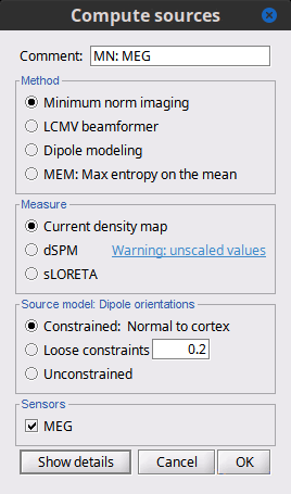
Minimum-norm (MN) imaging
- MN imaging estimates the amplitude of brain sources distributed across the brain or constrained to the cortex. The MN solution to the ill-posed EEG/MEG inverse problem is the one that best fits the sensor data with minimum overall amplitude of brain activity.
MN imaging requires the specification of noise statistics via a so-called noise covariance matrix. MEG users can best estimate noise statistics from an empty-room recording. If not available, as in EEG, noise covariance can be derived directly from recordings (e.g., from pre-stim segments, if relevant to the scientific question) or be assumed as uniform across sensors as described below.
Beamforming
- Brainstorm features the well-studied linearly constrained minimum variance (LCMV) beamformer to estimate source activity through a spatial filtering procedure. In lay terms, beamformer scans through all potential brain locations specified in the head model and estimates their respective contributions to sensor data, while attenuating the contributions from other brain regions.
Beamforming is technically similar to MN imaging, although it is more sensitive to approximations of the head model than MN imaging, and requires specific additional inputs. It is also blind to sources at different brain locations, but which time series are highly correlated.
LCMV beamformers require the specification of the data (noise+signal) covariance matrix, estimated directly from the recordings. LCMV source images can either be used as such, or post-processed, with a dipole model fitted at every time point of their largest peak(s). Please refer to the section further below for more detail about beamformers.
Dipole modeling
Brainstorm features a simple localization approach that adjusts the parameters of a single current dipole fitted to the sensor data at each point in time. As mentioned above, a LCMV-type map is first produced, and an equivalent current dipole is fitted at the strongest peak location of that map (more detail here).
Recommended option
- After exploring many, more sophisticated alternatives, our preference is to use simple and robust imaging approaches such as MN imaging or beamforming over single dipole scanning. However, this decision is often a matter of tradition in different resarch groups or subfields.
- Brainstorm enables the convenient comparison of these three approaches on your own data, with all possible sub-options, as detailed below.
MN imaging variants
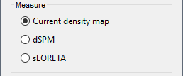
By default, MN imaging estimates the amplitude of brain electrical currents at each grid location determined by the forward head model (i.e., either in volume or on the cortical surface). As discussed here, the currents are expressed in A-m. Brainstorm does not normalize by surface area (A/m, i.e., current surface density) or volume (A/m^2, i.e., current volume density). Nonetheless, we refer to this default setting as yielding a current density map.
Current density map option: implements a L2-minimum norm estimate of brain current. FOr consistency, Brainstorm's method is identical to MNE's. Please refer to the MNE manual (Section 6, "The current estimates") for a technical description. Units are scaled to pA-m.
To further compensate for the inhomogenous sensitivity of EEG/MEG with depth and orientation of the current flow, we recommend that the current density maps obtained with this option be further standardized using a z-score transformation with respect to a specific time segment of no interest (e.g., pre-stimulus baseline) or experimental condition (e.g., resting-state).
Alternatively, such standardization can be achieved directly with respect to global noise and data covariance statistics via the dSPM and sLORETA options.
dSPM [recommended]: the derivations are those of the dynamical Statistical Parametric Mapping approach by Dale et al. (2000), based on the default MN option above adn scaled with respect to the noise covariance. The resulting dSPM maps are a set of z-scores. Units: unitless "z".
sLORETA: is the Standardized LOw Resolution brain Electromagnetic TomogrAphy approach by Pasqual-Marqui (2002). The default current density maps are normalized with respect to anestimate of the data covariance, derived as the sum of the noise covariance and a model of brain signal covariance (see original paper for detail). Note that the sLORETA data covariance is not the empirical data covariance estimated directly from the data, as used in beamformers). Units: unitless.
Source model: Dipole orientations [TODO]
The current flow of neural activity at each source localtion is modeled by the orientation of an equivalent current dipole. Brainstorm features the following options to determine this orientation:
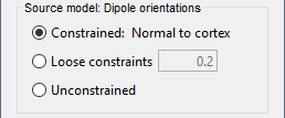
Constrained: Normal to cortex: this option is available only when working with "surface" grid locations (such as the cortical surface). Current dipoles are oriented normally to the cortical surface, to model the orientation of macrocolumns of pyramidal neurons perpendicular to the cortex.
Size of the imaging kernel: [Nvertices x Nchannels].Loose: This option is available only when working with "surface" grid locations (such as the cortical surface). In addition to a dipole normal to cortex as above, two additional dipoles are adeed in the tangential plane at each cortical location. Their amplitude is constrained below a fraction of the main normal dipole's. The recommended values are between 0.1 and 0.6. This option relaxes the constraint of strict orientation to the cortex to account for anatomical and physiological uncertainties.
Size of the imaging kernel: [3*Nvertices x Nchannels].Unconstrained: This option is available for both "surface" and "volume" source grids. There are 3 orthogonal dipoles at each grid location along the x, y, and z ("Cartesian") directions of the coordinate system.
Size of the imaging kernel: [3*Nvertices x Nchannels].Recommended option: The fully constrained option require only one dipole per source grid location, instead of three. Therefore, the source and kernel files are smaller, faster to compute and display. However, when using MRI templates instead of individual anatomy, loose/unconstrained orientation models may account for some of the model uncertainties (see this section).
Sensors

Brainstorm automatically detects the type of sensors (mEg, EEG, etc.) available from the head model selected for source imaging. In the example above, only MEG sensors are available. Select one or all the sensor types available you are interested in.
However, cross-modality calculations -- the fusion between MEG and EEG data to yield a joint source map -- are very sensitive to covariance calculations and head model approximations. As of Spring of 2018, we have also elected to NOT account for cross-covariances between different sensor types. If you wish to obtain a joint, multimodal source model, we recommend that you compute each source map separately and then combine them visually or quantitatively.
Computing sources for an average
We describe here a basic example of how to use Brainstorm to obtain a MN imaging maps of event-related average sensor data.
In Run#01, right-click on the average response for the deviant stim > Compute sources [2018].
Select the options: Minimum norm imaging, Current density map, Constrained: Normal to cortex.
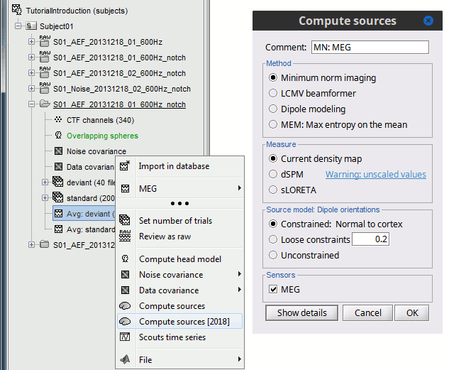 (The other "Compute sources" menu is for legacy options and implementations of the same imaging options.)
 The outcome of this process is a new dependent file of the sensor data, indicated with a brain icon. The file label (aka "comment") indicates "MN", which stands for "minimum-norm", and "Constr", which stands for "Constrained: normal orientation".
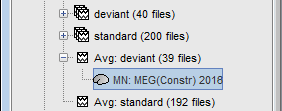
Display: Cortex surface
Right-click on this new source file with the brain icon and select > Cortical activations > Display on cortex.
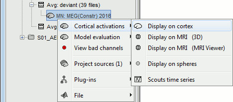
Double-click on the recordings for the deviant average to display the sensor time series alongside their brain source maps.
In the filter tab, add a low-pass filter at 40Hz to smooth the time series a bit.
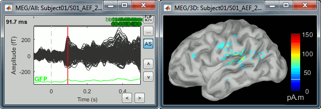
- Note how the display of the sensor and brain map windows are sync'd in time (click anywhere in the white portion of the time series window or use the left/right keyboard arrows to change the time stamp). You can also use all the menus and shortcuts introduced in the anatomy tutorial to use pre-set displays (0-6 keys).
Edit the display properties of the brain map in the Surface tab:
Amplitude: applies a minimum threshold to the source amplitude values displayed. The threshold is defined as a percentage ratio of the maximum amplitude value of the currrent color scale.
Min size: removes the smaller clusters in the source map, which number of source is smaller than the "min size" value entered.
Transparency: changes the opacity of the source map on the cortex surface.
Note that these parameters only adjust the visualization of source maps. They do not have effect on the actual source time series.
A few more words about the amplitude threshold parameter:
The maximum of the current colorbar depends on the Sources colormap parameters. If "Maximum: Global" is selected, the maximum indicated should be around 150 pA.m in the present dataset. This value represents the maximum of the source map across the entire dataset (across space and time). You can change the colorbar maximum value with the colormap option "Maximum: Custom".
On the screen capture below, the threshold value is set to 20%: only sources with amplitudes greater than 0.20*150 = 30 pA.m are shown.
The threshold value is shown in the colorbar with a horizontal white line.In the current data example, the source map should indicate strong activations around the primary auditory cortex around 91ms, bilaterally.
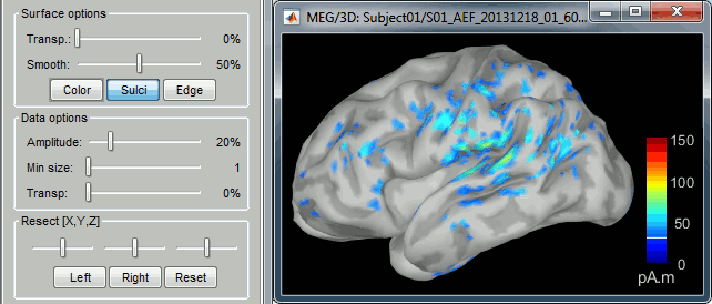
Recommended post-processing steps
The original source maps may look noisy or patchy. This is due to the strict orientation constraint used in the brain mapping procedure, which emphasizes the sensitivity of brain current strengths to the curvature of the cortex (this effect is more pronounced with MEG than EEG).
Please be cautious not to interpret disconnected colored patches as distinct brain activations without further post processing. The absolute spatial resolution of MEG source mapping is limited (~5-10mm, worse in EEG), although its relative resolution between experimental conditions, hence with post processing, can be much finer (1mm or less, see for instance this retinotopy study).
For now, you may generate smoother versions of the source maps by applying a spatial smoothing process (process "Sources > Spatial smoothing"), or using unconstrained source models, or standardizing source amplitude by applying a z-score transformation with respect to a time period of reference.
Brain maps obtained with dSPM or sLORETA are also standardize, more immune to orientation confounds (see below for more detail).
Display: MRI Viewer
Right-click on the source file for the deviant average > Cortical activations > Display on MRI (MRI Viewer).
See Brainstorm's MRI Viewer detailed tutorial in Sections #2 and #3.
This display shows cortical source activity interpolated in the the MRI volume. Set the amplitude threshold to 0% to visualize the cortex ribbon used onto which source activity is mapped.
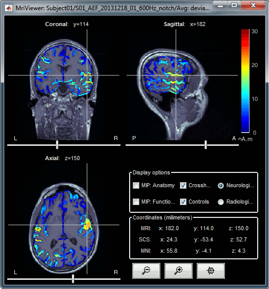
- Visualization parameters:
MIP Anatomy: check this box to obtain a "glass brain" view of the structural MRI, across all three spatial dimensions. MIP stands for "Maximum Intensity Projection"
MIP Functional: to obtain a glass brain view of the source map.
Amplitude threshold: in the Surface tab of the main Brainstorm window, to apply a threshold on the source map, as explained for the 3-D cortex view above.
Current time: shows the current time stamp in the data recordings, at the top-right of the main Brainstorm window. You also use the right/left arrows to move in time, or click anywhere in the white area of the sensor time series window.
Overlay options: Right-on the figure to get access additional options.
Smooth: Increase this value to smooth the source map further, for visualization purposes. This parameter defines the size of the smoothing kernel, in number of voxels.
Interpolation sources>MRI: Parameters to compute the interpolation on the MRI volume of the source maps, available on a source space of 15000 points located on the cortex surface. This procedure associates to each of the millions of MRI voxels a value computed from these 15000 source values. This menu lets you control some parameters of this interpolation.
Interpolate values: If enabled, performs a distance-weighted interpolation with 3 nearest neighbors (default for source results). If disable, performs a single nearest-neighbor lookup instead (useful to represent integer values that should not be interpolated, such as parcel labels).
Distance threshold: Maximum distance between a colored voxel and a grid point.
Resolution: Spatial resolution of the interpolated source maps. By default, the interpolation computes a source volume downsampled by a factor 3 with respect to the anatomical MRI, in order to make the computation faster. In that case, each colored element has a dimension of 3x3x3 voxels. If a higher resolution is needed (e.g. for displaying SEEG data) this parameter can be lowered to 1 or 2 voxels. Using a 1-voxel resolution requires the computation of 3*3*3=27 times more voxel values than with the default option, leading to much longer computation times.
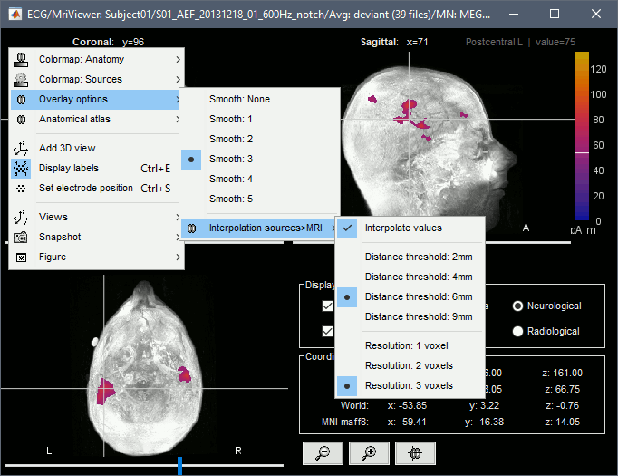
Display: MRI 3D
Right-click on the source file for the deviant average > Cortical activations > Display on MRI (3D).
We detailed this feature in the previous tutorial sections about MRI and surface visualization.
Keep right mouse button pressed and move the mouse to change the MR slices displayed. You can also use the Resect panel of the Surface tab.
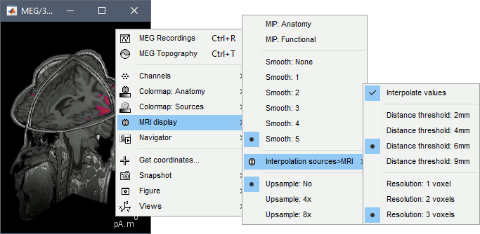
Sign of constrained maps
Source brain maps consist of time series that are complex curves of positive and negative values.
You can visualize how the sign of source amplitudes is distributed across the cortex using the cortical display of sources: set the amplitude threshold to 0%, then make sure the colormap shows relative (i.e., both positive and negative) values. For this, right click over the colorbar Colormap: Sources > uncheck the "Absolute values" option. At any time, you can double-click on the colorbar to reset the colormap options to default values.
As shown below, a typical brain map will show stripes of positive and negative values, with sign changes around sulcal locations. This is another manifestation of the limited absolute spatial resolution of MEG/EEG source mapping. Sources of opposite sides of sulcus are oriented in opposite directions by default. Source mapping shows they have oppositive signs meaning that the respective neural currents are estimated as flowing in the same direction. We will see later how this sign ambiguity can be managed via either the processing of rectified source time series (if you wish to map source amplitude effects only). It is crucial to preserve the sign though if you are in interested in frequency specific brain activity, such as spectral, time-frequency and connectivity analyses.
More on sign ambiguity: On opposite walls of a sulcus, brain source are very close to each other, with opposite orientations. If the true brain activity sits only on one side of a sulcus as shown below with a green arrow, the MN-imaging brain map lower spatial resolution will spread the estimated currents over multiple nearby locations, shown with the red and blue arrows below, which have opposite default directions that are imposed by anatomy (dipoles pointing outwards the cortical surface). The signs of the current flows will be opposite, with positive values (red arrows) on one side of the sulcus and negative values on the other side (blue arrows).
For visualization purposes, we are mostly interested at this stage in visualizing the magnitude of brain activity, hence the default colormap option "absolute values" being selected.
Unconstrained orientations
The "loose constraints" and "unconstrained" options for source orientations yield 3 time series per brain location (from three orthogonal elementary sources), which increases the dimensionality of the source maps, hence complexify their interpretation, but produces smoother renderings of current flows. We recommend these options when using an MRI template instead of the individual MRI volume of study participants, or when studying subcortical brain structures. Unconstrained maps can subsequently be converted to "flat" maps with a single orientation per location.
Here we will illustrate the fully unconstrained case. The procedure for the loose constraints options is similar.
In Run#01, right-click on the trial average of the deviant condition > Compute sources [2018].
Select the options: Minimum norm imaging, Current density map, Unconstrained.Double-click on the source file produced (brain icon, labelled with "Unconstr") and on the corresponding sensor data file. The two brain maps below represent the same file at 91ms, with different colormap options (absolute values on the left, relative values on the right). Explanations below.
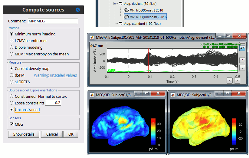
Again, using unconstrained/loose source orientations consists of triplets of dipoles with orthogonal orientations at each cortex location. To display their activity in a visually-meaningful manner, we first need to reduce the dimensions of the source data and color code the outcome. Brainstorm displays the norm of the vectorial sum of the three orientations at each vertex.
S = sqrt(Sx2 + Sy2 + Sz2)

This explains that only positive values are displayed over the source map. Note that the actual full values along each orientation (x,y,z) are signed and can be retrieved from the source file for further derivations (e.g., spectral analyses).
- The unconstrained/loose orientation maps are typically smoother than with the constrained orientation option (but see post-processing steps below) because they are less overly sensitive to changes in the curvature of the cortex.
You may delete the unconstrained source file: we will not use this option further in the introduction tutorials. Please refer to the tutorial EEG and epilepsy for further exploration of this option.
Standardization of source maps
Standardization procedures can compensate some of the bias of MN imaging source maps towards superficial source locations (in both MEG and EEG) and radially oriented current flows (in MEG). It also enables a fairer comparison of brain activity between individuals, based on its relative change with a data segment of reference.
Reference data segments can be extracted from empty-room recordings (MEG), pre-stimulus baseline or resting state data (MEG and EEG).
dSPM and sLORETA proceed to such standardization within their respective source mapping procedures. Brainstorm also features a Z-score normalization process, which enables a versatile definition of the reference data segment.
Source map standardization does not alter the dynamics of the source time series and only scales their respective amplitude changes. The scaling factors are different at each brain location, hence the resulting source maps will look different than the original MN images, but with the same temporal dynamics.
dSPM, sLORETA (embedded standardization)
In Run#01, right-click on the average sensor data of the deviant condition > Compute sources [2018].
Select successively the two normalization options: dSPM, sLORETA, (constrained).

Double-click on all the resulting source files to compare them (screen capture below is at the 143-ms time point):

Current density maps (MN imaging): without further standardization, MN imaging tends be biased towards the most superficial gyral crowns (see Z-score procedure below).
dSPM: compensates some of this bias. The amplitude of brain maps are converted to z-scores. You may adjust the z-scores with the number of trials used to obtain the sample average via specific process "Sources > Scale averaged dSPM" (see Averaging normalized values).
sLORETA: also produces unitless maps, but the statistics are proper to the method and therefore, are not related to z-scores.
Z-score transformation of brain maps
The Z-transformation of MN imaging brain maps centre source amplitudes around their mean over a reference segment, and scale them with respect to their standard deviation over the same reference segment: Z = (Data - μ) / σ
- The mean and standard deviation parameters are estimated from the data and are specific of each source location. Hence, sources with lower fluctuations over the reference segment (e.g., with less noise, or overall smaller amplitude) will be boosted by the transformation.
In Process1: Select the constrained current density map (file MN: MEG(Constr)).
Run process "Standardize > Baseline normalization", [-100,-1.7]ms, Z-score transformation
Do not select "Use absolute values" as for now, we wish to preserve the sign of source amplitudes.
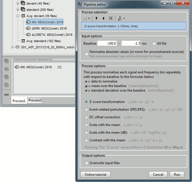
Double-click on the new brain map file (with the "| zscore" tag).

- We can appreciate that the standardized map is now qualitatively similar to dSPM and sLORETA versions.
- A map value of 3 means that the source amplitude at this time point is 3 times above the typical amplitude of that same source during the reference segment.
Please note Brainstorm's online filters do not affect the z-transformed source maps. Using the Filter tab and applying a bandpass filter will update the display all sensor time series and source maps on display, except the z-transormed maps.
If you wish to use a reference segment from another data file (e.g., a resting state recording as reference for the current task recording), use the Process2 process tab by dragging and dropping the reference source map in the Files A list on the left, and the source maps to be standardized in the Files B list on the right.
Recommended options
Use non-standardized current density maps (MN imaging) for:
- Computing imaging kernels shared across single trials.
- Averaging files across several MEG/EEG runs.
- Deriving spectral, time-frequency decompositions, phase-amplitude, or connectivity measures on single trials.
Use standardized maps (dSPM, sLORETA, Z-score) for:
- Producing source maps of trial averages (ERP/ERF).
- Before running a group analysis of source maps.
- Recommended standardization approach:
- dSPM and sLORETA are convenient linear measures which are easy to manipulate with Brainstorm.
- sLORETA maps are spatially smoother but with no direct statistical interpretation without further inference testing.
- dSPM and Z-score maps are statistically interpretable as excursions with respect to a reference data segment (Z-score), or with respect to noise covariance statistics (dSPM).
Delete your experiments
Before we proceed with the rest of the tutorial, please delete the source maps computed so far.
Select all the source files you computed until now and delete them.
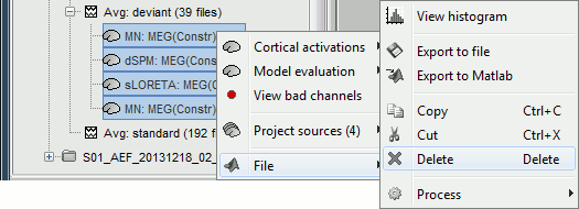
Computing sources for single trials
MN imaging models are linear: their respective imaging kernels can be pre-computed from anatomy and sensor locations only, then can be applied at once on long, ongoing or several epoched data segments on the fly. Here we show how to obtain source maps across multiple single trial epochs.
Right-click on the head model or the folder for Run#01 > Compute sources [2018].
Select: Minimum norm imaging, Current density map, Constrained: Normal to cortex
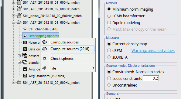
This procedure produces a shared imaging kernel (white brain icon) that is comon to all data files in Run #01. If you right-click on this new file, a warning message pops up that says "Inversion kernel". This file does not contain source maps, only the linear operator (kernel) to convert the sensor data into source maps.
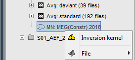
All data files in Run #01 (averages and single epochs) now show a link to a source file (grey brain icon), which is a virtual brain map that is computed on the fly when visualized: Brainstorm multiplies the imaging kernel by the sensor data time series, for greater computational and data storage efficacy. You may now visualize and manipulate these virtual source maps just like the maps we computed above.
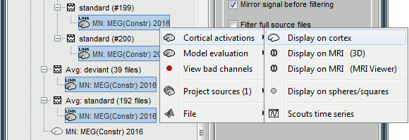
Averaging in source space
Computing the average
First compute the same source model for the the second acquisition run.
In Run#02, right-click on the head model or the folder > Compute sources [2018].
Select: Minimum norm imaging, Current density map, Constrained: Normal to cortex
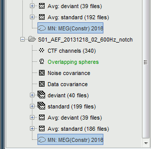
Now we have the source maps available for all the recordings, we can average them in source space across runs. This allows us to average MEG recordings that were recorded with different head positions (in this case Run#01 and Run#02 have different channel files so they could potentially have different head positions preventing the direct averaging at the sensor level).
Thanks to the linearity of the minimum norm model: MN(Average(trials)) = Average(MN(trials))
The two following approaches are equivalent:- Averaging the sources of all the individual trials across runs,
- Averaging the sources for the sensor averages that we already computed for each run.
- We will use the second option: using the sources for the sensor-level averages. It is a lot faster because it needs to read 4 files (one average file per run and per condition) instead of 456 files (total number of good trials in the two runs).
Drag and drop to the Process1 tab the average recordings for Run01 and Run02, then press the [Process sources] button on the left to select the source files instead of the MEG recordings.
Run process "Average > Average files":
Select "By trial group (subject average)" to average together files with similar names.
Select "Arithmetic average" function.
Check "Weighted average" to account for the different numbers of trials in both runs.
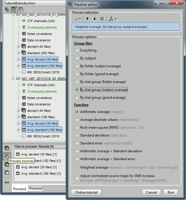
The two averages that are produced (one for each condition) are saved in the folder Intra-subject. This is where all the files computed using information from multiple folders within the same subject are saved. If you prefer to have them somewhere else, you can create new folders and move them there, just like you would do with a regular file explorer.
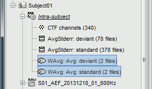
The file comments say "2 files" because they were computed from two averages each (one from each run), but the number of corresponding trials is correctly updated in the file structure.
Right-click on each of them > File > View file contents, and check the Leff field:
78 trials for the deviant condition, 378 trials for the standard condition.Double-click on the source averages to display them (deviant=top, standard=bottom).
Open the sensor-level averages as a time reference.
Use the predefined view "Left, Right" for looking at the two sides at the same time (shortcut: "7").
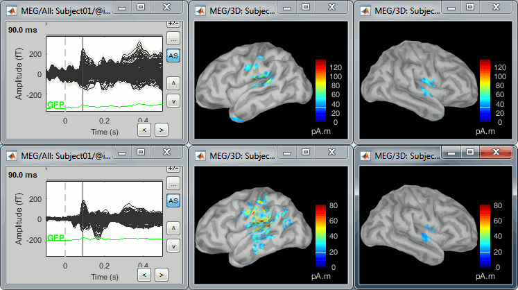
Visualization filters
Note that opening the source maps can be very long because of the filters for visualization. Check in the Filter tab, you may have a filter applied with the option "Filter all results" selected. In the case of averaged source maps, the 15,000 source signals are filtered on the fly when you load a source file. This filtering of the full source files can take a significant amount of time, consider unchecking this option if the display is too slow on your computer.
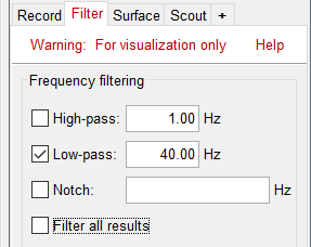
- It was not a problem until now because the source files were saved in the compact form (Kernel*recordings) and the visualization filters were applied on the recordings, then projected to the source space. This fast option is not available anymore with these averages across runs.
- The visualization filters will not be available anymore after we apply a Z-score normalization. If we want to display Z-score source maps that are smoothed in time, we will have to apply explicitly the filters on the file, with the Process1 tab.
Low-pass filter
- Clear the Process1 list, then drag and drop the new averages in it.
Run process "Pre-process > Band-pass filter": [0,40] Hz
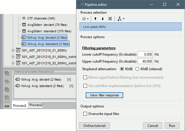
Epochs are too short: Look at the filter response, the expected transient duration is at least 78ms. The first and last 78ms of the average should be discarded after filtering. However, doing this would get rid of almost all the 100ms baseline, which we need for normalization. As mentioned here, we should have been importing longer epochs in order to filter and normalize the averages properly.
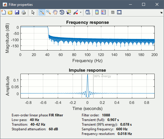
Z-score normalization
- In Process1, select the two filtered averages.
Run process "Standardize > Baseline normalization", baseline=[-100,-1.7]ms, Z-score.
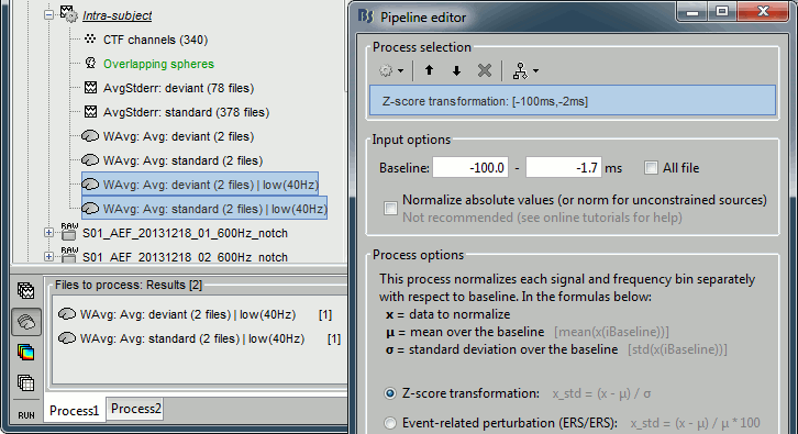
Four new files are accessible in the database: two filtered and two filtered+normalized.
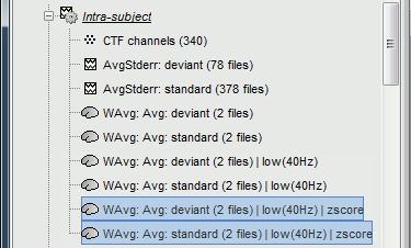
Double-click on the source averages to display them (deviant=top, standard=bottom).
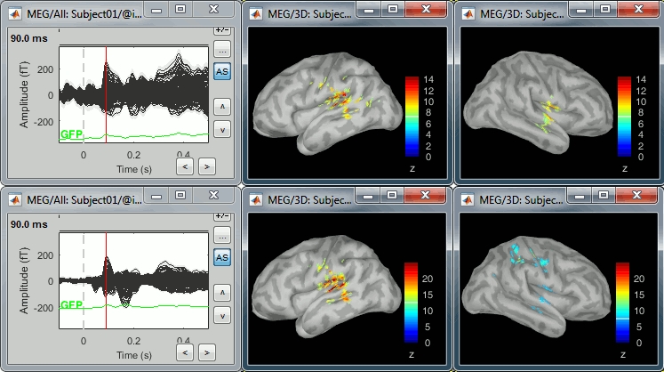
- The Z-score source values at 90ms are higher for the standard condition (~25) than for the deviant condition (~15). We observe this because the two conditions have very different signal-to-noise ratios. The standard condition has about 5x more trials, therefore the standard deviation over the baseline is a lot lower, leading to higher Z-score.
Delete the non-normalized filtered files, we will not use them in the following tutorials.
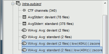
Note for beginners
Everything below is advanced documentation, you can skip it for now.
Averaging normalized values
Averaging normalized source maps within a single subject requires more attention than averaging current density maps. Since averaging reduces variance, the resulting source maps will have a different statistical distribution than the nominal distribution of the individual maps.
For example, averaging z-score normalized maps will result in maps with variance less than 1. The same holds true for dSPM maps. Assuming independent samples, the variance of an average of N maps drops by 1/N. For this reason, it is generally recommended to select the "Weighted average" option in the ‘Average files’ process when averaging trials or source maps (which performs mean(x) = (N1*sum(x1(i)) + N2*sum(x2(i)) + …)/ (N1+N2+…) ) in order to keep track of the number of samples and the actual variance of averaged statistical maps.
dSPM
- An averaged dSPM map has variance equal to 1/N (and thus standard deviation equal to 1/sqrt(N)). Therefore one could multiply the averaged dSPM map by sqrt(N) in order to maintain variance 1 under the null hypothesis. In previous versions of Brainstorm, this was done automatically when visualizing the files, and when averaging source maps with the option "Adjust normalized source maps for SNR increase". To simplify the interface and make the interpretation of maps more intuitive and consistent with other cases (min-norm, z-scored), we now dropped this option. Thus averaging dSPM maps now results in maps with variance less than 1, and is consistent with handling min-norm, z-scored and sLORETA maps.
Ajusting an averaged dSPM file by this sqrt(N) factor is still possible manually, eg. in order to visualize cortical maps that can be interpreted as Z values. Select the average dSPM files in Process1 and run process "Sources > Scale averaged dSPM". This should be used only for visualization and interpretation, scaled dSPM should never be averaged or used for any other statistical analysis.
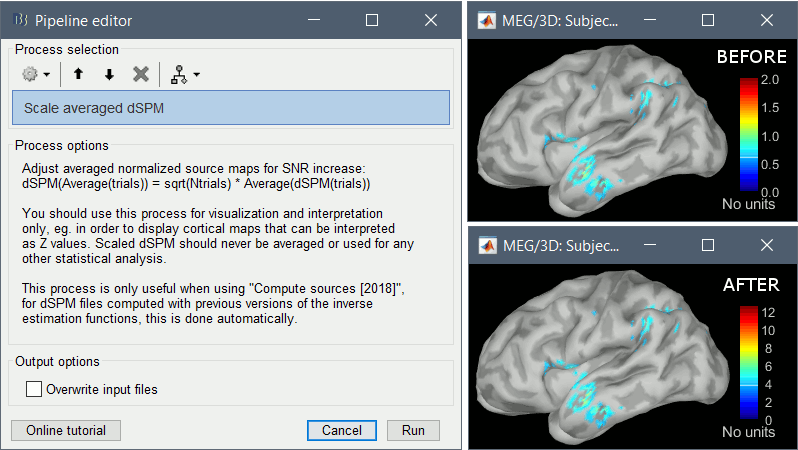
Z-score
- The same SNR issues arise while averaging Z-scores: the average of the Z-scores is lower than the Z-score of the average.
When computing averages at the subject level: Always avoid averaging Z-score maps.
Average the current density maps, then normalize.
sLORETA
- This normalization is not based on the SNR of signal, but rather on the spatial smoothness of the maps. Managing these maps is similar to min-norm maps: the variance of the individual maps is not explicitly modeled or known analytically.
- As in other cases, sLORETA(Average(trials)) = Average(sLORETA(trials)), and this relationship is guaranteed to hold with averaging uneven number of samples when using the option "Weighted average".
Display: Contact sheets and movies
A good way to represent what is happening in time is to generate contact sheets or videos. Right-click on any figure and go to the menu Snapshot to check out all the possible options. For a nicer result, take some time to adjust the size of the figure, the amplitude threshold and the colormap options (hiding the colorbar can be a good option for contact sheets).
A time stamp is added to the captured figure. The size of the text font is fixed, so if you want it to be readable in the contact sheet, you should make you figure very small before starting the capture. The screen captures below where produced with the colormap "hot".
Contact sheet: Right-click on any figure > Snapshot > Time contact sheet: Figure
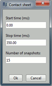
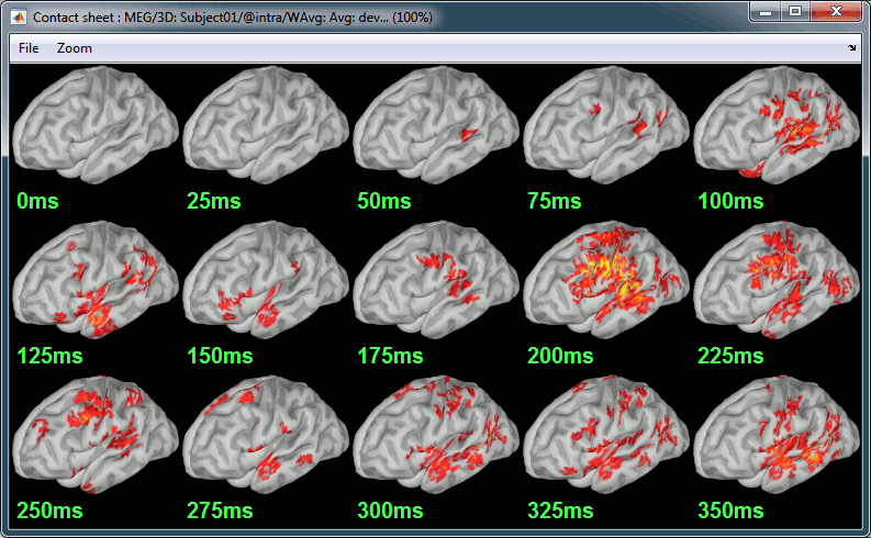
Movies: Right-click on any figure > Snapshot > Movie (time): All figures
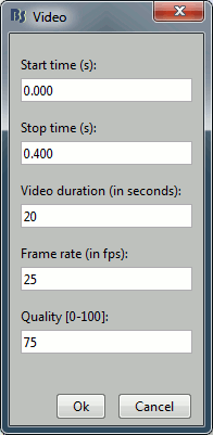
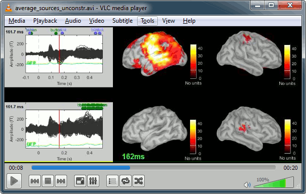
Model evaluation
One way to evaluate the accuracy of the source reconstruction if to simulate recordings using the estimated source maps. This is done simply by multiplying the source time series with the forward model:
MEG_simulated [Nmeg x Ntime] = Forward_model [Nmeg x Nsources] * MN_sources [Nsources x Ntime]
Then you can compare visually the original MEG recordings with the simulated ones. More formally, you can compute an error measure from the residuals (recordings - simulated).
To simulate MEG recordings from a minimum norm source model, right-click on the source file, then select the menu "Model evaluation > Simulate recordings".
Open side-by-side the original and simulated MEG recordings for the same condition:
Advanced options: Minimum norm
Right-click on the deviant average for Run#01 > Compute sources [2018].
Click on the button [Show details] to bring up all the advanced minimum norm options.
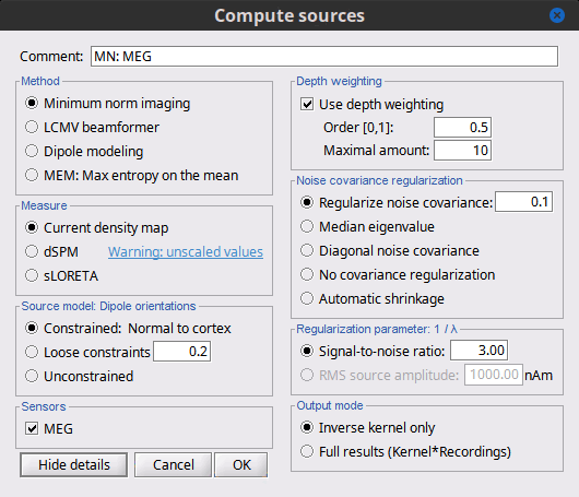
Depth weighting
Briefly, the use of various depth weightings was far more debated in the 1990s, before the introduction of MNE normalization via dSPM, sLORETA, and other "z-scoring" methods, which mostly cancel the effects of depth weighting (put another way, after normalization min norm results tend to look quite similar whether depth weighting is used or not).
By modifying the source covariance model at each point in the source grid, deeper sources are "boosted" to increase their signal strength relative to the shallower dipoles; otherwise, the resulting MNE current density maps are too dominated by the shallower sources. If using dSPM or sLORETA, little difference in using depth weighting should be noted. To understand how to set these parameters, please refer to the MNE manual. (options --depth, --weightexp and --weightlimit).
Noise covariance regularization [TODO]
MNE and dipole modeling are best done with an accurate model of the noise covariance, which is generally computed from experimental data. As such, these estimates are themselves prone to errors that arise from relatively too few data points, weak sensors, and strange data dependencies that can cause the eigenspectrum of the covariance matrix to be illconditioned (i.e. a large eigenvalue spread or matrix condition number). In Brainstorm, we provide several means to "stabilize" or "regularize" the noise covariance matrix, so that source estimation calculations are more robust to small errors.
Regularize noise covariance: The L2 matrix norm is defined as the largest eigenvalue of its eigenspectrum. This option adds to the covariance matrix a diagonal matrix whos entries are a fraction of the matrix norm. The default is 0.1, such that covariance matrix is stabilized by adding to it an identity matrix that is scaled to 10% of the largest eigenvalue.
Median eigenvalue: The eigenspectrum of MEG data can often span many decades, due to highly colored spatial noise, but this broad spectrum is generally confined to the first several modes only. Thus the L2 norm is many times greater than the majority of the eigenvalues, and it is difficult to prescribe a conventional regularization parameter. Instability in the inverse is dominated by defects found in the smallest eigenvalues. This approach stabilizes the eigenspectrum by replicating the median (middle) eigenvalue for the remainder of the small eigenvalues.
Diagonal noise covariance: Deficiencies in the eigenspectrum often arise from numerical inter-dependencies found among the channels, particularly in covariance matrices computed from relatively short sequences of data. One common method of stabilization is to simply take the diagonal of the covariance matrix and zero-out the cross-covariances. Each channel is therefore modeled as independent of the other channels. The eigenspectrum is now simply the (sorted) diagonal values.
No covariance regularization: We simply use the noise covariance matrix as computed or provided by the user.
Automatic shrinkage: Stabilization method of Ledoit and Wolf (2004), still under testing in the Brainstorm environment. Basically tries to estimate a good tradeoff between no regularization and diagonal regularization, using a "shrinkage" factor. See Brainstorm code "bst_inverse_linear_2018.m" for notes and details.
Recommended option: This author (Mosher) votes for the median eigenvalue as being generally effective. The other options are useful for comparing with other software packages that generally employ similar regularization methods. [TODO]
Regularization parameter [TODO]
In minimum norm estimates, as mentioned above in the comparisons among methods, the data covariance matrix is essentially synthesized by adding the noise covariance matrix to a modeled signal covariance matrix. The signal covariance matrix is generated by passing the source prior through the forward model. The source prior is in turn prescribed by the source model orientation and the depth weighting.
A final regularization parameter, however, determines how much weight the signal model should be given relative to the noise model, i.e. the "signal to noise ratio" (SNR). In Brainstorm, we follow the definition of SNR as first defined in the original MNE software of Hamalainen. The signal covariance matrix is "whitened" by the noise covariance matrix, such that the whitened eigenspectrum has elements in terms of SNR (power). We find the mean of this spectrum, then take the square root to yield the average SNR (amplitude). The default in MNE and in Brainstorm is "3", i.e. the average SNR (power) is 9.
Signal-to-noise ratio: Use SNR of 3 as the classic recommendation, as discussed above.
RMS source amplitude: An alternative definition of SNR, but still under test and may be dropped. [TODO]
Output mode
As mentioned above, these methods create a convenient linear imaging kernel that is "tall" in the number of elemental dipoles (one or three per grid point) and "wide" only in the number of sensors. At subsequent visualization time, we efficiently multiply the kernel with the data matrix to compute the min norm images.
For some custom purposes, however, a user may find it convenient to pre-multiply the data matrix and generate the full source estimation matrix. This would only be recommended in small data sets, since the full results can become quite large.
Kernel only: Saves only the linear inverse operator, a model that converts sensor values into source values. The size of this matrix is: number of sources (15000) x number of MEG sensors (274). The multiplication with the recordings is done on the fly by Brainstorm in a transparent way. For long recordings or numerous epochs, this form of compact storage helps saving a lot of disk space and computation time, and it speeds up significantly the display. Always select this option when possible.
Full results: Saves in one big matrix the values of all the sources (15,000) for all the time samples (361). The size in memory of such a matrix is about 45Mb for 600ms of recordings. This is still reasonable, so you may use this option in this case. But if you need to process longer recordings, you may face "Out of memory" errors in Matlab, or fill your hard drive quickly.
- Full results [15000x361] = Inverse kernel [15000x274] * Recordings [274x361]
Advanced options: LCMV beamformer
As mentioned in the introduction above, two other methods can be selected for source estimation, a beamformer and dipole modeling. In this section, we review the options for the beamformer. On top of the noise covariance matrix, you need to estimate a data covariance matrix in order to enable the option "LCMV beamformer" in the interface.
Note that pre-whitening with the noise covariance matrix has not yet been implemented for the LCMV beamformer, and only the data covariance is used in the current version. The noise covariance has no impact on the LCMV beamformer results. However, if there is no noise covariance file available in the database, the "Compute sources" interface returns an error: to go around this limitation, you may select the "No noise modeling (identity matrix)" option in the contextual menu for the noise covariance.
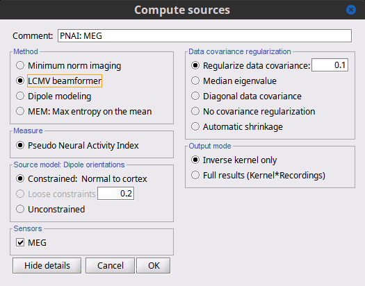
Measure
The only option "Pseudo Neural Activity Index" (PNAI), is named after the definition of the Neural Activity Index (NAI). We have modified Van Veen’s definition to rely strictly on the data covariance, without need for a separate noise covariance matrix, but the basic premise is the same as in dSPM, sLORETA, and other normalizations. Viewing the resulting "map," in an identical manner to that with MNE, dSPM, and sLORETA described above, reveals possibly multiple sources as peaks in the map. Note that PNAI scores are unitless, because they correspond to standardized statistical fluctuations of neural currents. In this way, PNAI scores are analogous to z-scoring.
Dipole orientations
We recommend you choose "unconstrained" and let the later Dipole scanning process, which finds the best fitting dipole at each time point, optimize the orientation with respect to the data.
Data covariance regularization
Same definitions as in MNE, only applied to the data covariance matrix, rather than the noise covariance matrix. Our recommendation is to use median eigenvalue.
Advanced options: Dipole modeling
Dipole modeling fits a single dipole at each potential source location to produce a dipole scanning map. This map can be viewed as a indication of how well, and where, the dipole fits at each time point. However, we recommend using the subsequent best-dipole fitting routine (dipole scanning) to determine the final location and orientation of the dipole (one per time point). Please note that this function does not fit multiple simultaneous dipoles.
Although not widely recognized, dipole modeling and beamforming are more alike than they are different – when comparing the inverse operators required to compute the dipole scanning map (dipole modeling) and the beamformer output map (LCMV), we see that they differ only in that the former uses an inverse noise covariance matrix while the latter replaces this with the inverse of the data covariance.
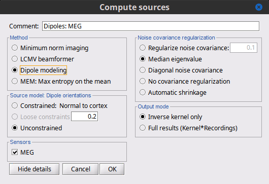
Measure
This field is now missing, but the resulting imaging kernel file is directly analogous to the PNAI result from LCMV beamforming. The user can display this scanning measure just as with the LCMV case, where again the normalization and units are a form of z-scoring.
Dipole orientations
Use "unconstrained source" modeling and let the process "dipole scanning" optimize the orientation of the dipole for every time instance.
Noise covariance regularization
Similarly, use "median eigenvalue".
The tutorial "MEG current phantom (Elekta)" demonstrates dipole modeling of 32 individual dipoles under realistic experimental noise conditions.
Combining MEG+EEG for source estimation
Magnetoencephalography and EEG sensor data can be processed jointly to produce combined source estimates. Joint processing presents unique challenges because EEG and MEG use head models that exhibit differing sensitivities to modeling errors, which can in turn lead to inconsistencies between EEG and MEG with respect to the (common) source model. In practice joint processing is relatively rare (Baillet et al., 1999). However, these data are complementary, which means that joint processing can potentially yield insights that cannot be seen with either modality alone.
For example, in the evoked responses in the data set used here, the first peak over the occipital areas is observed in MEG (90 ms) slightly before EEG (110 ms). This delay is too large to be caused by acquisition imprecisions. This indicates that we are not capturing the same brain processes with the two modalities, possibly because the orientation and type of activity in the underlying cortical sources is different.
MEG and EEG have different sensitivities to source orientation and depth. Given the challenges of joint processing, our advice is to first look at the source reconstructions for the two modalities separately before trying to use any type of fusion technique.
On the hard drive
Constrained shared kernel
Right-click on a shared inverse file in the database explorer > File > View file contents.
Structure of the source files: results_*.mat
Mandatory fields:
ImagingKernel: Linear inverse operator that must be multiplied by the recordings in order to get the full source time series. If defined, ImageGridAmp must be empty.
- Size for constrained sources [Nsources x Nchannels]
- Size for unconstrained sources [3xNsources x Nchannels]. Order of sources: source1.x, source1.y, source1.z, ... sourceN.z)
ImageGridAmp: Full source time series, in Amper.meter. If this field is defined, ImagingKernel must be empty. If you want this field to be set instead of ImagingKernel, make sure you select the advanced option Full results when estimating the sources.
- Size for constrained sources [Nsources x Ntime]
- Size for unconstrained sources [3xNsources x Ntime]. Order of sources: source1.x, source1.y, source1.z, ... sourceN.z)
Time: [1 x Ntime] Time values for each sample recorded in F, in seconds.
nComponents: Number of dipoles per grid point: 1=Constrained, 3=Unconstrained, 0=Mixed. In the case of mixed head models, the atlas GridAtlas documents region by region how the list of grid points matches the list of dipoles.
Function: Type of values currently saved in the file: 'mn', 'mnp', 'dspm', 'dspm2018', 'dspm2018sc', 'sloreta', 'lcmv', 'lcmvp', 'lcmvnai', 'lcmvpow', 'gls', 'glsp', 'glsfit', 'glschi', 'zscore', 'ersd'...
HeadModelType: Type of source space used for this head model ('surface', 'volume', 'mixed').
HeadModelFile: Relative path to the head model used to compute the sources.
SurfaceFile: Relative path to the cortex surface file related with this head model.
Atlas: Used only by the process "Sources > Downsample to atlas".
GridLoc: [Nvertices x 3], (x,y,z) positions of the grid of source points. In the case of a surface head model, it is empty and you read directly the positions from the surface file.
GridOrient: [Nvertices x 3], direction of the normal to the surface for each vertex point (copy of the 'VertNormals' matrix of the cortex surface). Empty in the case of a volume head model or unconstrained sources.
GridAtlas: Atlas "Source model" used with mixed source models.
GoodChannel: [1 x Nchannels] Array of channel indices used to estimate the sources.
DataFile: Relative path to the recordings file for which the sources where computed. If this field is set, the source file appears as a dependent of the DataFile.
Comment: String displayed in the database explorer to represent this file.
History: Operations performed on the file since it was create (menu "View file history").
Optional fields:
Options: Structure that contains all the options of the inverse calculation. This is saved in the file only for bookkeeping.
Whitener: Noise covariance whitener computed in bst_inverse_linear_2018.m
DataWhitener: Data covariance whitener computed in bst_inverse_linear_2018.m
SourceDecompVa: [3 x Nsources] Concatenated right singular vectors from the SVD decomposition of the whitened leadfield for each source (only for unconstrained sources).
SourceDecompSa: [3 x Nvertices] Vector diagonal of the singular values from the SVD decomposition of the whitened leadfield for each source (only for unconstrained sources).
Std: For averaged files, number of trials that were used to compute this file.
DisplayUnits: String, force the display of this file using a specific type of units.
ChannelFlag: [Nchannels x 1] Copy of the ChannelFlag field from the original data file.
Leff: Effective number of averages. For averaged files, number of trials that were used to compute this file. For source files that are attached to a data file, we use the Leff field from the data file.
Full source maps
In Intra-subject, right-click on one of the normalized averages > File > View file contents.
This file has the same structure as a shared inverse kernel, with the following differences:
It contains the full time series (ImageGridAmp) instead of an inverse operator (ImagingKernel).
The Z-score process updated the field Function ('mn' => 'zscore')
Source links
- The links are not real files on the hard drive, if you select the menu "View file contents" for any of them it would display the structure of the corresponding shared kernel.
They are saved in the database as strings with a specific structure: "link|kernel_file|data_file". This string associates a shared inverse operator with some recordings. The two files have to be available to load the this file. All the functions in Brainstorm are equipped to reconstruct the full source matrix dynamically.
Filename tags
_KERNEL_: Indicates that the file contains only an inverse kernel, it needs to be associated with recordings to be opened.
Useful functions
in_bst_results(ResultsFile, LoadFull, FieldsList): Load a source file and optionally reconstruct the full source time series on the fly (ImagingKernel * recordings).
in_bst(FileName, TimeBounds, LoadFull): Load any Brainstorm data file with the possibility to load only a specific part of the file.
bst_process('LoadInputFile', FileName, Target, TimeWindow, OPTIONS): The most high-level function for reading data files, can compute scout values on the fly.
Additional documentation
Articles
Minimum norm: Baillet S, Mosher JC, Leahy RM
Electromagnetic brain mapping, IEEE SP MAG 2001.dSPM: Dale AM, Liu AK, Fischl BR, Buckner RL, Belliveau JW, Lewine JD, Halgren E
Dynamic statistical parametric mapping: combining fMRI and MEG for high-resolution imaging of cortical activity. Neuron 2000 Apr, 26(1):55-67sLORETA: Pascual-Marqui RD
Standardized low-resolution brain electromagnetic tomography (sLORETA): technical details, Methods Find Exp Clin Pharmacol 2002, 24 Suppl D:5-12LCMV Beamformer:
Jaiswal A, Nenonen J, Stenroos M, Gramfort A, Dalal SS, Westner BU, Litvak V, Mosher JC, Schoffelen JM, Witton C, Oostenveld R,
Comparison of beamformer implementations for MEG source localization,
Neuroimage. 2020 Aug 1, 216: 116797
Westner BU, Dalal SS, Gramfort A, Litvak V, Mosher JC, Oostenveld R, Schoffelen JM
A unified view on beamformers for M/EEG source reconstruction,
NeuroImage. 2022 Feb 1;246:118789
Tutorials
Tutorial: Volume source estimation
Tutorial: Deep cerebral structures
Tutorial: Computing and displaying dipoles
Tutorial: Dipole fitting with FieldTrip
Tutorial: Maximum Entropy on the Mean (MEM)
Forum discussions
Forum: Minimum norm units (pA.m): http://neuroimage.usc.edu/forums/showthread.php?1246
Forum: Imaging resolution kernels: http://neuroimage.usc.edu/forums/showthread.php?1298
Forum: Spatial smoothing: http://neuroimage.usc.edu/forums/showthread.php?1409
Forum: Units for dSPM/sLORETA: http://neuroimage.usc.edu/forums/showthread.php?1535
Forum: EEG reference: http://neuroimage.usc.edu/forums/showthread.php?1525#post6718
Forum: Sign of the MNE values: http://neuroimage.usc.edu/forums/showthread.php?1649
Forum: Combine MEG+EEG: https://neuroimage.usc.edu/forums/t/1684
Forum: Combine mag+gradiometers: http://neuroimage.usc.edu/forums/showthread.php?1900
Forum: Combine EEG+fMRI: http://neuroimage.usc.edu/forums/showthread.php?2679
Forum: Residual ocular artifacts: http://neuroimage.usc.edu/forums/showthread.php?1272
Forum: Dipole fitting: http://neuroimage.usc.edu/forums/showthread.php?2400
Forum: Dipole scanning and goodness of fit: https://neuroimage.usc.edu/forums/t/33645
Forum: Simulate recordings from sources: http://neuroimage.usc.edu/forums/showthread.php?2563
Forum: Simulate recordings from simulated signals: https://neuroimage.usc.edu/forums/t/2421
Forum: Pre-whitening: https://neuroimage.usc.edu/forums/t/10459
Forum: Adjustment of SNR option: https://neuroimage.usc.edu/forums/t/36817
Forum: LCMV beamformer and noise covariance: https://neuroimage.usc.edu/forums/t/30943
Forum: Debugging weird sLORETA results: https://neuroimage.usc.edu/forums/t/21265
Forum: Subset of sensors: https://neuroimage.usc.edu/forums/t/26496


