Contents
- Tutorial 1: Create a new protocol
- Tutorial 2: Import the subject anatomy
- Tutorial 3: Display the anatomy
- Tutorial 4: Channel file / MEG-MRI coregistration
- Tutorial 5: Review continuous recordings
- Tutorial 6: Multiple windows
- Tutorial 7: Event markers
- Tutorial 8: Stimulation delays
- Tutorial 9: Select files and run processes
- Tutorial 10: Power spectrum and frequency filters
- Tutorial 11: Bad channels
- Tutorial 12: Artifact detection
- Tutorial 13: Artifact cleaning with SSP
- Tutorial 14: Additional bad segments
- Tutorial 15: Import epochs
- Tutorial 16: Average response
- Tutorial 17: Visual exploration
- Tutorial 18: Colormaps
- Tutorial 19: Clusters of sensors
- Tutorial 20: Head modeling
- Tutorial 21: Noise and data covariance matrices
- Tutorial 22: Source estimation
- Tutorial 23: Scouts
- Tutorial 24: Time-frequency
- Tutorial 26: Statistics
- Tutorial 27: Workflows
- Tutorial 28: Scripting
Tutorial 1: Create a new protocol
Authors: Francois Tadel, Elizabeth Bock, Sylvain Baillet
Contents
- How to read these tutorials
- Presentation of the experiment
- Brainstorm folders
- Starting Brainstorm for the first time
- Main interface window
- The text is too small
- Database structure
- Database files
- Create your first protocol
- Protocol exploration
- Set up a backup
- Changing the temporary folder
- Summary
- Roadmap
- Moving a database
How to read these tutorials
The goal of these introduction tutorials is to guide you through most of the features of the software. All the pages use the same example dataset. The results of one section are most of the time used in the following section, so read these pages in the correct order.
Some pages may contain too many details for your level of interest or competence. The sections marked as [Advanced] are not required for you to follow the tutorials until the end. You can skip them the first time you go through the documentation. You will be able to get back to the theory later if you need.
Please follow first these tutorials with the data we provide. This way you will be able to focus on learning how to use the software. It is better to start with some data that is easy to analyze. After going through all the tutorials, you should be comfortable enough with the software to start analyzing your own recordings.
You will observe minor differences between the screen captures presented in these pages and what you obtain on your computer: different colormaps, different values, etc. The software being constantly improved, some results changed since we produced the illustrations. When the changes are minor and the interpretation of the figures remain the same, we don't necessarily update the images in the tutorial.
If you are interested only in EEG or intra-cranial recordings, don't think that a MEG-based tutorial is not adapted for you. Most of the practical aspects of the data manipulation is very similar in EEG and MEG. First start by reading these introduction tutorials using the MEG example dataset provided, then when you are familiar with the software, go through the tutorial "EEG and Epilepsy" to get some more details about the processing steps that are specific for EEG, or read one of the SEEG/ECOG tutorials available in the section "Other analysis scenarios".
Presentation of the experiment
All the introduction tutorials are based on a simple auditory oddball experiment:
- One subject, two acquisition runs of 6 minutes each.
- Subject stimulated binaurally with intra-aural earphones.
- Each run contains 200 regular beeps and 40 easy deviant beeps.
- Recordings with a CTF MEG system with 275 axial gradiometers.
Anatomy of the subject: 1.5T MRI, processed with FreeSurfer 5.3.
- More details will be given about this dataset along the process.
Full dataset description available on this page: Introduction dataset.
Brainstorm folders
Brainstorm needs different directories to work properly. If you put everything in the same folder, you would run into many problems. Try to understand this organization before creating a new database.
1. Program directory: "brainstorm3"
- Contains all the program files: Matlab scripts, compiled binaries, templates, etc.
- There is no user data in this folder.
- You can delete it and replace it with a newer version at anytime, your data will be safe.
- Recommended location:
Windows: Documents\brainstorm3
Linux: /home/username/brainstorm3
MacOS: Documents/brainstorm3
2. Database directory: "brainstorm_db"
- Created by user.
- Contains all the Brainstorm database files.
- Managed by the application: do not move, delete or add files by yourself.
- Recommended location:
Windows: Documents\brainstorm_db
Linux: /home/username/brainstorm_db
MacOS: Documents/brainstorm_db
3. User directory: ".brainstorm"
Created at Brainstorm startup. Typical location:
Windows: C:\Users\username\.brainstorm
Linux: /home/username/.brainstorm
MacOS: /Users/username/.brainstorm
- Contains:
brainstorm.mat: Brainstorm user preferences.
defaults/: Anatomy templates downloaded by Brainstorm.
mex/: Some mex files that have to be recompiled.
plugins/: Plugins downloaded by Brainstorm (see tutorial Plugins).
process/: Personal process folder (see tutorial How to write your own process).
reports/: Execution reports (see tutorial Run processes).
tmp/: Temporary folder, emptied every time Brainstorm is started with user confirmation.
You may have to change the location of the temporary folder if you have a limited amount of storage or a limited quota in your home folder (see below).
Be sure that the paths to the Program, Database, and User directories do not contain special characters. See related forum post.
4. Original data files:
- Recordings you acquired and you want to process with Brainstorm.
Put them wherever you want but not in any of the previous folders.
Starting Brainstorm for the first time
If you haven't read the installation instructions, do it now: Installation.
Start Brainstorm from Matlab or with the compiled executable.
BST> Starting Brainstorm:
BST> =================================
BST> Version: 28-Jan-2015
BST> Checking internet connectivity... ok
BST> Compiling main interface files...
BST> Emptying temporary directory...
BST> Deleting old process reports...
BST> Loading configuration file...
BST> Initializing user interface...
BST> Starting OpenGL engine... hardware
BST> Reading plugins folder...
BST> Loading current protocol...
BST> =================================
- Read and accept the license file.
- Select your Brainstorm database directory (brainstorm_db).
If you do something wrong and don't know how to go back, you can always re-initialize Brainstorm by typing "brainstorm reset" in the Matlab command window, or by clicking on [Reset] in the software preferences (menu File > Edit preferences).
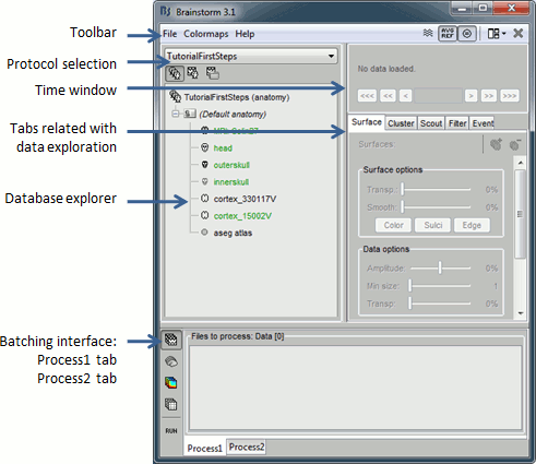
Main interface window
The Brainstorm window described below is designed to remain on one side of the screen. All the space of the desktop that is not covered by this window will be used for opening other figures.
Do not try to maximize this window, or the automatic management of the data figures might not work correctly. Keep it on one side of your screen, just large enough so you can read the file names in the database explorer.
The text is too small
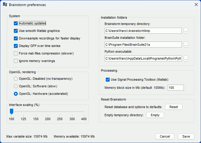
If you have a high-resolution screen, the text and icons in the Brainstorm window may not scale properly, leading the interface to be impossible to use. Select the menu File > Edit preferences, the slider at the bottom of the option window lets you increase the ratio of the Brainstorm interface. If it doesn't help, try changing the scaling options in your operating system preferences.
Database structure
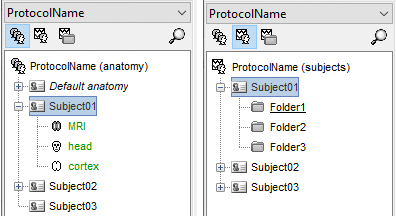
Brainstorm allows you to organize your recordings and analysis with three levels of definition:
Protocol
- Group of datasets that have to be processed or displayed together.
- A protocol can include one or several subjects.
Some people would prefer to call this experiment or study.
- You can only open one protocol at a time.
- Your Brainstorm database is a collection of protocols.
Subject
- A person who participated in a given protocol.
- A subject contains two categories of information: anatomy and functional data.
Anatomy: Includes at least an MRI volume and some surfaces extracted from the MRI.
Functional data: Everything that is related with the MEG/EEG acquisition.
- For each subject, it is possible to use either the actual MRI of the person or one of the anatomy templates available in Brainstorm.
Sub-folders
- For each subject, the functional files can be organized in different sub-folders.
- These folders can represent different recordings sessions (aka acquisition runs) or different experimental conditions.
The current structure of the database does not allow more than one level of sub-folders for each subject. It is not possible to organize the files by session AND by condition.
Database files
- The database folder "brainstorm_db" is managed completely from the graphic user interface (GUI).
- All the files in the database have to be imported through the GUI. Do not try to copy files by yourself in the brainstorm_db folder, it won't work.
- Everything in this folder is stored in Matlab .mat format, with the following architecture:
Anatomy data: brainstorm_db/protocol_name/anat/subject_name
Functional data: brainstorm_db/protocol_name/data/subject_name/subfolder/
- Most of the files you see in the database explorer in Brainstorm correspond to files on the hard drive, but there is no one-to-one correspondence. There is extra information stored in each directory, to save properties, comments, default data, links between different items, etc. This is one of the reasons for which you should not try to manipulate directly the files in the Brainstorm database directory.
- The structure of the database is saved in the user preferences, so when you start the program or change protocol, there is no need to read again all the files on the hard drive.
If Brainstorm or Matlab crashes before the database structure is correctly saved, the files that are displayed in the Brainstorm database explorer may differ from what is actually on the disk. When this happens, you can force Brainstorm to rebuild the structure from the files on the hard drive: right-click on a folder > Reload.
Create your first protocol
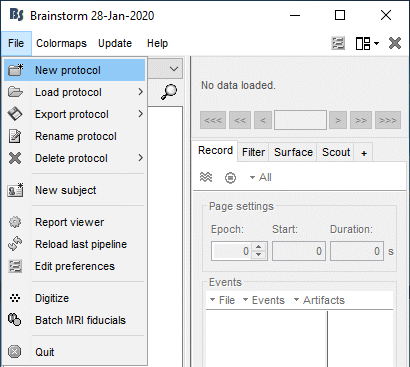
Menu File > New protocol.
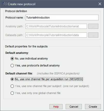
Edit the protocol name and enter: "TutorialIntroduction".
It will automatically update the anatomy and datasets paths. Do not edit manually these paths, unless you work with a non-standard database organization and know exactly what you are doing.- Default properties for the subjects: These are the default settings that are used when creating new subjects. It is then possible to override these settings for each subject individually.
Default anatomy: (MRI and surfaces)
No, use individual anatomy:
Select when you have individual MRI scans for all the participants of your study.Yes, use default anatomy:
Select when you do not have individual scans for the participants, and you would like to use one of the anatomy templates available in Brainstorm.
Default channel file: (Sensors names and positions)
No, use one channel file per acquisition run: Default for all studies
Different head positions: Select this if you may have different head positions for one subject. This is usually not the case in EEG, where the electrodes stay in place for all the experiment. In MEG, this is a common setting: one recording session is split in multiple acquisition runs, and the position of the subject's head in the MEG might be different between two runs.
Different number of channels: Another use case is when you have multiple recordings for the same subject that do not have the same number of channels. You cannot share the channel file if the list of channels is not strictly the same for all the files.
Different cleaning procedures: If you are cleaning artifacts from each acquisition run separately using SSP or ICA projectors, you cannot share the channel file between them (the projectors are saved in the channel file).Yes, use one channel file per subject: Use with caution
This can be a setting adapted to EEG: the electrodes are in the same position for all the files recorded on one subject, and the number of channels is the same for all the files. However, to use this option, you should not be using SSP/ICA projectors on the recordings, or they should be computed for all the files at once. This may lead to some confusion and sometimes to manipulation errors. For this reason, we decided not to recommend this setting.Yes, use only one global channel file: Not recommended
This is never a recommended setting. It could be used in the case of an EEG study where you use only standard EEG positions on a standard anatomy, but only if you are not doing any advanced source reconstruction. If you share the position of the electrodes between all the subjects, it will also share the source models, which are dependent on the quality of the recordings for each subject. This is complicated to understand at this level, it will make more sense later in the tutorials.
In the context of this study, we are going to use the following settings:
No, use individual anatomy: Because we have access to a T1 MRI scan of the subject.
No, use one channel file per condition/run: The typical MEG setup.
Click on [Create].
Protocol exploration
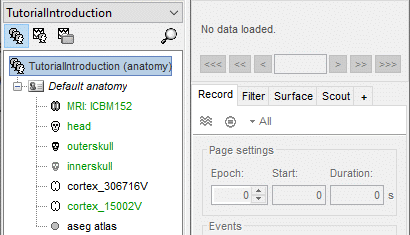
The protocol is created and you can now see it in the database explorer. It is represented by the top-most node in the tree.
- You can switch between anatomy and functional data with the three buttons just above the database explorer. Read the tooltips of the buttons to see which one does what.
In the Anatomy view, there is a Default anatomy node. It contains the ICBM152 anatomy, distributed by the Montreal Neurological Institute (MNI), which is one of the template anatomy folders that are distributed with Brainstorm.
The Default anatomy node contains the MRI and the surfaces that are used for the subjects without an individual anatomy, or for registering multiple subjects to the same anatomy for group analysis.
There are no subjects in the database yet, so the Functional data views are empty.
Everything you can do with an object in the database explorer (anatomy files, subjects, protocol) is accessible by right-clicking on it.
Set up a backup
Just like any computer work, your Brainstorm database is always at risk. Software bugs, computer or network crashes and manipulation errors can cause the loss of months of data curation and computation. If the database structure gets corrupted or if you delete or modify accidentally some files, you might not be able to get your data back. There is no undo button!
You created your database, now take some time to find a way to make it safe. If you are not familiar with backuping systems, watch some online tutorials explaining how to set up an automatic daily or weekly backup of your sensitive data. It might seem annoying and useless now, but could save you weeks in the future.
Changing the temporary folder
Some processes need to create temporary files on the hard drive. For example, when epoching MEG/EEG recordings, Brainstorm would first create a temporary folder "import_yymmdd_hhmmss", store all the epochs in it, then move them to the database when the epoching process is completed. The name of the temporary folder indicates its creation time (year/month/day_hour_minutes_seconds). At the end of the process, all the temporary files should be deleted automatically.
The default folder where Brainstorm stores its temporary files is located in the user folder ($HOME/.brainstorm/tmp/), so before importing recordings or calculating large models, you have to make sure you have enough storage space available.
If you work on a centralized network where all the computers are sharing the same resources, the system admins may impose limited disk quotas to all users and encourage them to use local hard drives instead of the limited and shared user folder. In such context, Brainstorm may quickly fill up your limited quota and at some point block your user account.
If the amount of storage space you have for your user folder is limited (less than 10Gb), you may have to change the temporary folder used by Brainstorm. Select the menu File > Edit preferences and set the temporary directory to a folder that is local to your computer, in which you won't suffer from any storage limitation.
If a process crashes or is killed before it deletes its temporary files, they would remain in the temporary folder until explicitly deleted. When starting Brainstorm, you would always get offered to delete the previous temporary files: always agree to it, unless they correspond to files generated by another session running simultaneously. Alternatively, you can delete these temporary files by clicking on the Empty button in the same preferences window. More information in the Scripting tutorial.

Summary
- Different folders for:
the program (brainstorm3).
the database (brainstorm_db).
your original recordings.
- Never modify the contents of the database folder by yourself.
- Do not put the original recordings in any of the Brainstorm folders, import them with the interface.
- Do not try to maximize the Brainstorm window: keep it small on one side of your screen.
Roadmap
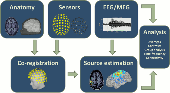
The workflow described in these introduction tutorials include the following steps:
- Importing the anatomy of the subjects, the definition of the sensors and the recordings.
- Pre-processing, cleaning, epoching and averaging the EEG/MEG recordings.
- Estimating sources from the imported recordings.
- Computing measures from the brain signals of interest in sensor space or source space.
Moving a database
If you are running out of disk space or need to share your database with someone else, you may need to copy or move your protocols to a different folder or drive. Each protocol is handled independently by Brainstorm, therefore in order to move the entire database folder (brainstorm_db), you need to repeat the operations below for each protocol in your database.
Copy the raw files
The original continuous files are not saved in the Brainstorm database. The "Link to raw files" depend on a static path on your local computer and cannot be moved easily to a new computer. You can copy them inside the database before moving the database to a different computer/hard drive using the menu: File > Export protocol > Copy raw files to database. This will make local copies in .bst format of all your original files. The resulting protocol would be larger but portable. This can also be done file by file: right-click > File > Copy to database.
Export a protocol
The easiest option to share a protocol with a collaborator is to export it as a zip file.
Export: Use the menu File > Export protocol > Export as zip file.
Avoid using spaces and special characters in the zip file name.Import: Use the menu File > Load protocol > Load from zip file.
The name of the protocol created in the brainstorm_db folder is the name of the zip file. If there is already a protocol with this label, Brainstorm would return an error. To import the protocol as a different name, you only need to rename the zip file before importing it.Size limitation: This solution is limited to smaller databases: creating zip files larger than a few Gb can take a lot of time or even crash. For larger databases, prefer the other options below.
Export a subject
Similar as the protocol export, but extracts only the files needed by a single subject.
Export: Right-click on the subject > File > Export subject.
Import as new protocol: Use the menu File > Load protocol > Load from zip file.
Import in an existing protocol: Use the menu File > Load protocol > Import subject from zip.
Move a protocol
To move a protocol to a different location:
- [Optional] Set up a backup of your entire brainstorm_db folder if your haven't done it yet. There will be no undo button to press if something bad happens.
- [Optional] Copy the raw files to the database (see above)
Unload: Menu File > Delete protocol > Only detach from database.
Move: Move the entire protocol folder to a different location. Remember a protocol folder should be located in the "brainstorm_db" folder and should contain only two subfolders "data" and "anat". Never move or copy a single subject manually.
Load: Menu File > Load protocol > Load from folder > Select the new location of the protocol
- If you want to move the entire "brainstorm_db" folder at once, make sure you detach all the protocols in your Brainstorm installation first.
Duplicate a protocol
To duplicate a protocol in the same computer:
Copy: Make a full copy of the protocol to duplicate in the brainstorm_db folder, e.g. TutorialIntroduction => TutorialIntroduction_copy. Avoid using any space or special character in the new folder name.
Load: Menu File > Load protocol > Load from folder > Select the new protocol folder
Tutorial 2: Import the subject anatomy
Authors: Francois Tadel, Elizabeth Bock, Sylvain Baillet, Chinmay Chinara
Brainstorm orients most of its database organization and processing stream for handling anatomical information together with the MEG/EEG recordings, because its primary focus was to estimate brain sources from MEG/EEG, which ideally requires an accurate spatial modelling of the head and sensors.
If you don't have anatomical scans of your subjects or are not interested in any spatial display, various solution will be presented along the tutorials, starting from the last section of this page. Be patient and follow everything as instructed, you will get to the information you need.
Contents
Download
The dataset we will use for the introduction tutorials is available online.
Go to the Download page of this website, and download the file: sample_introduction.zip
- Unzip it in a folder that is not in any of the Brainstorm folders (program folder or database folder).
- This is really important that you always keep your original data files in a separate folder: the program folder can be deleted when updating the software, and the contents of the database folder is supposed to be manipulated only by the program itself.
Create a new subject
The protocol is currently empty. You need to add a new subject before you can start importing data.
- Switch to the anatomy view (first button just above the database explorer).
Right-click on the top folder TutorialIntroduction > New subject.
Alternatively: Use the menu File > New subject.
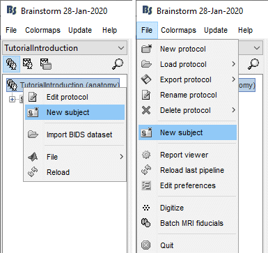
The window that opens lets you edit the subject name and settings. It offers again the same options for the default anatomy and channel file: you can redefine for one subject the default values set at the protocol level if you need to. See previous tutorial for help.
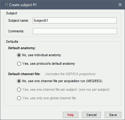
- Keep all the default settings and click on [Save].
Right-click doesn't work
If the right-click doesn't work anywhere in the Brainstorm interface and you cannot get to see the popup menus in the database explorer, try to connect a standard external mouse with two buttons. Some Apple pointing devices do not interact very well with Java/Matlab.
Alternatively, try to change the configuration of your trackpad in the system preferences.
Import the anatomy
For estimating the brain sources of the MEG/EEG signals, the anatomy of the subject must include at least three files: a T1-weighted MRI volume, the envelope of the cortex and the surface of the head.
Brainstorm cannot extract the cortex envelope from the MRI, you have to run this operation with an external program of your choice. The results of the MRI segmentation obtained with the following programs can be automatically imported: FreeSurfer, BrainSuite, BainVISA, CAT12, and CIVET. CAT is the only application fully interfaced with Brainstorm, and available for download as a Brainstorm plugin. However, FreeSurfer is more considered as a reference in this domain, therefore this is the solution we decided to demonstrate in these tutorials.
The anatomical information of this study was acquired with a 1.5T MRI scanner, the subject had a marker placed on the left cheek. The MRI volume was processed with FreeSurfer 7.1, the result of this automatic segmentation process is available in the downloaded folder sample_introduction/anatomy.
- Make sure that you are still in the anatomy view for your protocol.
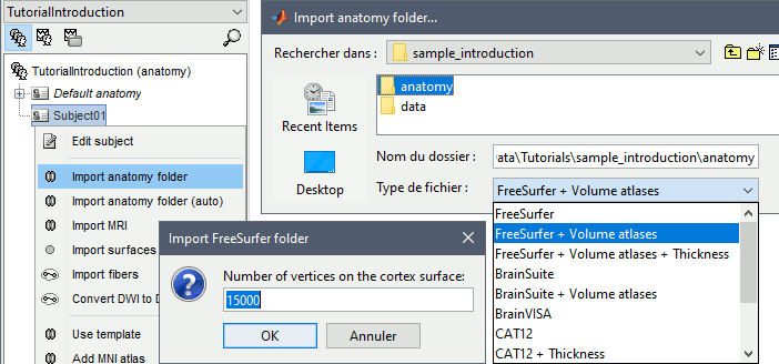
Right-click on the subject folder > Import anatomy folder:
Set the file format: FreeSurfer + Volume atlases
Select the folder: sample_introduction/anatomy
- Click on [Open]
Number of vertices of the cortex surface: 15000 (default value).
This option defines the number of points that will be used to represent the cortex envelope. It will also be the number of electric dipoles we will use to model the activity of the brain. This default value of 15000 was chosen empirically as a good balance between the spatial accuracy of the models and the computation speed. More details later in the tutorials.
The MRI views should be correct (axial/coronal/sagittal), you just need to make sure that the marker on the cheek is really on the left of the MRI. Then you can proceed with the fiducial selection.
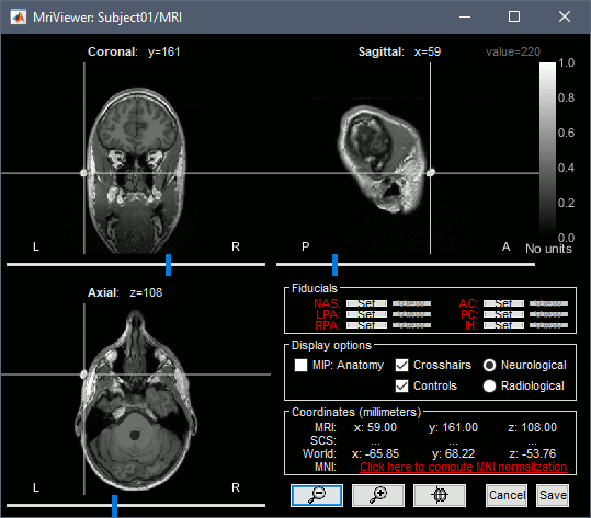
Using the MRI Viewer
To help define these fiducial points, let's start with a brief description of the MRI Viewer:
Navigate in the volume:
- Click anywhere on the MRI slices to move the cursor.
- Use the sliders below the views.
- Use the mouse wheel to scroll through slices (after clicking on the view to select it).
On a MacBook pad, use the two finger-move up/down to scroll.
Zoom: Use the magnifying glass buttons at the bottom of the figure, or the corresponding shortcuts (keyboard [+]/[-], or [CTRL]+mouse wheel).
Image contrast: Click and hold the right mouse button on one image, then move up and down.
Select a point: Place the cursor at the spot you want and click on the corresponding [Set] button.
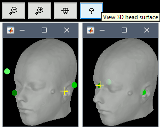
Display the head surface: Click on the button "View 3D head surface" to compute and display the head surface. Click on the surface to move the coordinates of the cursor in the MRI Viewer figure. When the fiducials are not defined, they appear as floating a few centimeters away from the head.
More information about all the coordinates displayed in this figure: CoordinateSystems
- Popup operations (right-click on the figure):
Colormap: Edit the colormap, detailed in another tutorial.
Anatomical atlas: Select, show and hide anatomical parcellations (aka anatomical atlases).
Views: Set one of the predefined orientation.
Apply MNI coordinates to all figures: Set the same MNI coordinates to other MRI viewer figures.
Apply SCS coordinates to all figures: Set the same SCS coordinates to other MRI viewer figures.
View in 3D orthogonal slices: Open MRI volume as 3D orthogonal slices, and set the same slices as in the MRI viewe.
Snapshots: Save images or movies from this figure.
Figure: Change some of the figure options or edit it using the Matlab tools.
- Note the indications in the right part of the popup menu, they represent the keyboard shortcut for each menu.
Fiducial points
Brainstorm uses a few reference points defined in the MRI to align the different files:
Required: Three points to define the Subject Coordinate System (SCS):
- Nasion (NAS), Left ear (LPA), Right ear (RPA)
- This is used to register the MEG/EEG sensors on the MRI.
Optional: Three additional anatomical landmarks (NCS):
- Anterior commissure (AC), Posterior commissure (PC) and any interhemispheric point (IH).
- Computing the MNI normalization sets these points automatically (see below), therefore setting them manually is not required.
For instructions on finding these points, read the following page: CoordinateSystems.
Nasion (NAS)
In this study, we used the real nasion position instead of the CTF coil position.

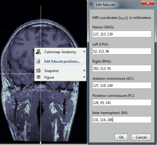
MRI coordinates: 127, 213, 139
Left ear (LPA)
In this study, we used the connection points between the tragus and the helix (red dot on the CoordinateSystems page) instead of the CTF coil position or the left and right preauricular points.

MRI coordinates: 52, 113, 96
Right ear (RPA)

MRI coordinates: 202, 113, 91
Anterior commissure (AC)

MRI coordinates: 127, 119, 149
Posterior commissure (PC)

MRI coordinates: 128, 93, 141
Inter-hemispheric point (IH)
This point can be anywhere in the mid-sagittal plane, these coordinates are just an example.

MRI coordinates: 131, 114, 206
Type the coordinates
If you have the coordinates of the fiducials already written somewhere, you can type or copy-paste them instead of the pointing at them in with the cursor. Right-click on the figure > Edit fiducials positions > MRI coordinates.
Validation
- Once you are done with the fiducial selection, click on the [Save] button, at the bottom-right corner of the MRI Viewer figure.
The automatic import of the FreeSurfer folder resumes. At the end you get many new files in the database and a 3D view of the cortex and scalp surface. Here again you can note that the marker is visible on the left cheek, as expected.

- The next tutorial will describe these files and explore the various visualization options.
Close all figures and clear memory: Use this button in the toolbar of the Brainstorm window to close all the open figures at once and to empty the memory from all the temporary data that the program keeps in memory for faster display.

Graphic bugs
If you do not see the cortex surface through the head surface, or if you observe any other issue with the 3D display, there might be an issue with the OpenGL drivers. You may try the following options:
- Update the drivers for your graphics card.
- Upgrade your version of Matlab.
Run the compiled version of Brainstorm (see Installation).
Turn off the OpenGL hardware acceleration: Menu File > Edit preferences > Software or Disabled.
Send a bug report to MathWorks.
For Linux users with an integrated GPU and NVIDIA GPU, if you experience the troubles above, or the slow navigation in the 3D display (usually with 2 or more surfaces). Verify that you are using the NVIDIA GPU as primary GPU. More information depending on your distribution: Ubuntu, Debian and Arch Linux.
MNI normalization
For comparing results with the literature or with other imaging modalities, the normalized MNI coordinate system is often used. To be able to get "MNI coordinates" for individual brains, an extra step of normalization is required.
To compute a transformation between the individual MRI and the ICBM152 space, you have two available options, use the one of your choice:
In the MRI Viewer: Click on the link "Click here to compute MNI normalization".
In the database explorer: Right-click on the MRI > MNI normalization.
Select the first option maff8: This method is embedded in Brainstorm and does not require the installation of SPM12. However, it requires the automatic download of the file SPM12 Tissue Probability Maps. If you do not have access to internet, see the instructions on the Installation page.
It is based on an affine co-registration with the MNI ICBM152 template from the SPM software, described in the following article: Ashburner J, Friston KJ, Unified segmentation, NeuroImage 2005.
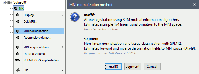
Note that this normalization does not modify the anatomy, it just saves a transformation that enables the conversion between Brainstorm coordinates and MNI coordinates. After computing this transformation, you have access to one new line of information in the MRI Viewer.
This operation also sets automatically some anatomical points (AC, PC, IH) if not defined yet. After the computation, make sure they are correctly positioned. You can run this computation while importing the anatomy, when the MRI viewer is displayed for the first time, this will save you the trouble of marking the AC/PC/IH points manually.
MacOS troubleshooting
Error "mexmaci64 cannot be opened because the developer cannot be verified":
Alternatives
The head surface looks bad: You can try computing another one with different properties.
No individual anatomy: If you do not have access to an individual MR scan of the subject, or if its quality is too low to be processed with FreeSurfer, you have other options:
If you do not have any individual anatomical data: Use the default anatomy
If you have a digitized head shape of the subject: Warp the default anatomy
Other options for importing the FreeSurfer anatomical segmentation:
Automated import: We selected the menu Import anatomy folder for a semi-manual import, in order to select manually the position of the anatomical fiducials and the number of points of the cortex surface. If you are not interested in setting accurately the positions of the fiducials, you can use the menu Import anatomy folder (auto): it computes the linear MNI normalization first and use default fiducials defined in MNI space, and uses automatically 15000 vertices for the cortex.
FreeSurfer options: We selected the file format FreeSurfer + Volume atlases for importing the ASEG parcellation in the database. This slows down the import and increases the size on the hard drive. If you know you won't use it, select FreeSurfer instead. A third menu is avalaible to also import the cortical thickness as source files in the database.
Tutorial 3: Display the anatomy
Authors: Francois Tadel, Elizabeth Bock, Sylvain Baillet
Contents
Anatomy folder
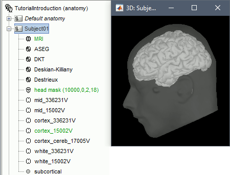
The anatomy of the subject "Subject01" should now contain all the files Brainstorm could import from the FreeSurfer segmentation results:
MRI: T1-weighted MRI, resampled and re-aligned by FreeSurfer.
ASEG / DKT / Desikan-Killiany / Destrieux: Volume parcellations (including subcortical regions)
Head mask: Head surface, generated by Brainstorm.
If this doesn't look good for your subject, you can recalculate another head surface using different parameters: right-click on the subject folder > Generate head surface.Cortex_336231V: High-resolution pial envelope generated by FreeSurfer.
Cortex_15002V: Low-resolution pial envelope, downsampled from the original one by Brainstorm.
Cortex_cereb_17005V: Low-res pial envelope + cerebellum surface extracted from ASEG
White_*: White matter envelope, high and low resolution.
Mid_*: Surface that represents the mid-point between the white and cortex envelopes.
Subcortical: Save FreeSurfer subcortical regions as in the ASEG volume, but tesselated as surfaces.
For more information about the files generated by FreeSurfer, read the FreeSurfer page.
Default surfaces
- There are four possible surface types: cortex, inner skull, outer skull, head.
- For each type of surface, one file is selected as the one to use by default for all the operations.
This selected surface is displayed in green.
- Here, there is only one "head" surface, which is selected.
The mid, cortex and white surfaces can all be used as "cortex" surfaces, only one can be selected at a time. By default, the low-resolution cortex should be selected and displayed in green.
To select a different cortex surface, you can double-click on it or right-click > Set as default.
MRI Viewer
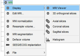
Right-click on the MRI to get the list of the available display menus:
Open the MRI Viewer. This interface was already introduced in the previous tutorial. It corresponds to the default display menu if you double-click on the MRI from the database explorer. Description of the window:
MIP Anatomy: Maximum Intensity Projection. When this option is selected, the MRI viewer shows the maximum intensity value across all the slices in each direction. This maximum does not depend on the selected slice, therefore if you move the cursor, the image stays the same.
Neurological/Radiological: There are two standard orientations for displaying medical scans. In the neurological orientation, the left hemisphere is on the left of the image, in the radiological orientation the left hemisphere is on the right of the image.
Coordinates: Position of the cursor in different coordinate systems. See: CoordinateSystems
Colormap: Click on the colorbar and move up/down (brightness) or left/right (contrast)
Popup menu: All the figures have additional options available in a popup menu, accessible with a right-click on the figure. The colormap options will be described later in the tutorials, you can test the other options by yourself.
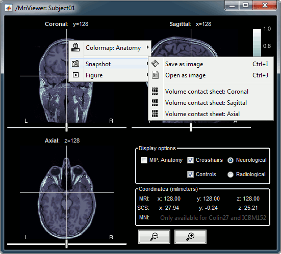
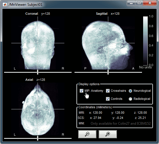
MRI contact sheets
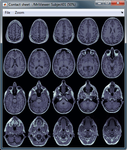
You can get collections of slices in any direction (axial, coronal or sagittal) with the popup menus in the database explorer or the MRI Viewer figure.
Zoom: mouse wheel (or two finger-move on a MacBook pad)
Move in zoomed image: click + move
Adjust contrast: right click + move up/down
MRI in 3D
Right-click on the MRI file in the database explorer > Display > 3D orthogonal slices.
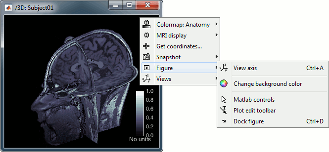
Simple mouse operations:
Rotate: Click + move. Note that two different types of rotations are available: at the center of the figure the object will follow you mouse, on the sides it will do a 2D rotation of the image.
Zoom: Mouse wheel, or two finger-move on a MacBook pad.
Move: Left+right click + move (or middle-click + move).
Colormap: Click on the colorbar and move up/down (brightness) or left/right (contrast).
Reset view: Double click anywhere on the figure.
Reset colormap: Double-click on the colorbar.
Move slices: Right click on the slice to move + move.
(or use the Resect panel in the Surface tab)
- Popup operations (right-click on the figure):
Colormap: Edit the colormap, detailed in another tutorial.
MRI display: For now, contains mostly the MIP option (Maximum Intensity Projection).
Get coordinates: Pick a point in any 3D view and get its coordinates.
Snapshots: Save images or movies from this figure.
Figure: Change some of the figure options or edit it using the Matlab tools.
Views: Set one of the predefined orientation.
- Note the indications in the right part of the popup menu, they represent the keyboard shortcut for each menu.
- Keyboard shortcuts:
Views shortcuts (0,1,2...9 and [=]): Remember them, they will be very useful when exploring the cortical sources. To switch from left to right, it is much faster to press a key than having to rotate the brain with the mouse.
Zoom: Keys [+] and [-] for zooming in and out.
Move slices: [x]=Sagittal, [y]=Coronal, [z]=Axial, hold [shift] for reverse direction.
- Surface tab (in the main Brainstorm window, right of the database explorer):
- This panel is primarily dedicated to the display of the surfaces, but some controls can also be useful for the 3D MRI view.
Transparency: Changes the transparency of the slices.
Smooth: Changes the background threshold applied to the MRI slices. If you set it zero, you will see the full slices, as extracted from the volume.
Resect: Changes the position of the slices in the three directions.
Surfaces
To display a surface you can either double-click on it or right-click > Display. The tab "Surface" contains buttons and sliders to control the display of the surfaces.
- The mouse and keyboard operations described for the 3D MRI view also apply here.
Smooth: Inflates the surface to make all the parts of the cortex envelope visible.
This is just a display option, it does not actually modify the surface.Color: Changes the color of the surface.
Sulci: Shows the bottom of the cortical folds with a darker color. We recommend to keep this option selected for the cortex, it helps for the interpretation of source locations on smoothed brains.
Edge: Display the faces of the surface tesselation.
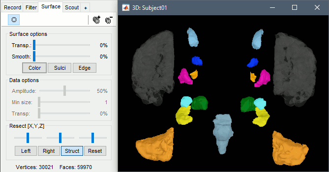
Resect: The sliders and the buttons Left/Right/Struct at the bottom of the panel allow you to cut the surface or reorganize the anatomical structures in various ways.
Multiple surfaces: If you open two surfaces from the same subject, they will be displayed on the same figure. Then you need to select the surface you want to edit before changing its properties. The list of available surfaces is displayed at the top of the Surface tab.
At the bottom of the Surface tab, you can read the number of vertices and faces in the tesselation.
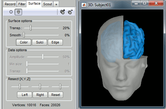
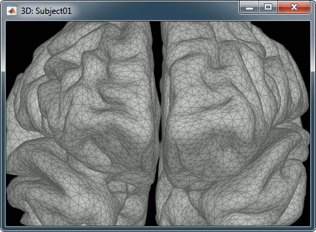
Get coordinates
- Close all the figures. Open the cortex surface again.
- Right-click on the 3D figure, select "Get coordinates".
- Click anywhere on the cortex surface: a yellow cross appears and the coordinates of the point are displayed in all the available coordinates systems.
You can click on [View/MRI] to see where this point is located in the MRI, using the MRI Viewer.
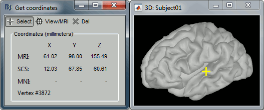
Subcortical regions: Volume
The standard FreeSurfer segmentation pipeline generates multiple volume parcellations of anatomical regions, all including the ASEG subcortical parcellation. Double-click on a volume parcellation to open it for display. This opens the MRI Viewer with two volumes: the T1 MRI as the background, and the parcellation as a semi-transparent overlay.
- Adjust the transparency of the overlay from the Surface tab, slider Transp.
The name of the region under the cursor appears at the top-right corner. The integer before this name is the label of the ROI, ie. the integer value of the voxel under the cursor in the parcellation volume.
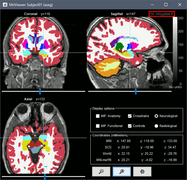
- Close the MRI viewer.
- Double-click again on the subject's MRI to open it in the MRI viewer.
- Observe that the anatomical label is also present at the top-right corner of this figure; in this case, the integer reprents the voxel value of the displayed MRI. This label information comes from the ASEG file: whenever there are volume parcellations available for the subject, one of them is loaded in the MRI Viewer by default. The name of the selected parcellation is displayed in the figure title bar.
You can change the selected parcellation with the right-click popup menu Anatomical atlas. You can change the parcellation scheme, disable its use to make the MRI work faster, or show the parcellation volume as an overlay (menu Show atlas). More information in the tutorial Using anatomy templates.

Subcortical regions: Surface
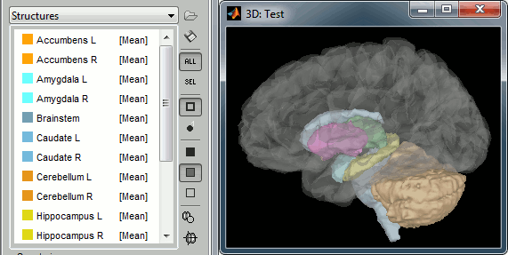
Brainstorm reads the ASEG volume labels and tesselates some of these regions, then groups all the meshes in a large surface file where the regions are identified in an atlas called "Structures". It identifies: 8 bilateral structures (accumbens, amygdala, caudate, hippocampus, pallidum, putamen, thalamus, cerebellum) and 1 central structure (brainstem).
These structures can be useful for advanced source modeling, but will not be used in the introduction tutorials. Please refer to the advanced tutorials for more information: Volume source estimation and Deep cerebral structures.
With the button [Struct] at the bottom of the Surface tab, you can see the structures separately.
Registration MRI/surfaces
The MRI and the surfaces are represented using the different coordinate systems and could be misregistered for various reasons. If you are using the automated segmentation pipeline from FreeSurfer or BrainSuite you should never have any problem, but if something goes wrong or in the case of more manual import procedures it is always good to check that the MRI and the surfaces are correctly aligned.
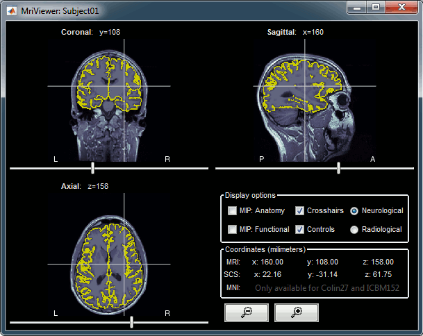
Right-click on the low-res cortex > MRI Registration > Check MRI/surface registration
- The calculation of the interpolation between the MRI and the cortex surface takes a few seconds, but the result is then saved in the database and will be reused later.
The yellow lines represent the re-interpolation of the surface in the MRI volume.
Interaction with the file system
For most manipulations, it is not necessary to know exactly what is going on at the level of the file system, in the Brainstorm database directory. However, many things are not accessible from the Brainstorm interface, you may sometimes find it useful to manipulate some piece of data directly from the Matlab command window.
Where are the files ?
- Leave your mouse for a few seconds over any node in the database explorer, a tooltip will appear with the name and path of the corresponding file on the hard drive.
Paths are relative to current protocol path (brainstorm_db/TutorialIntroduction). What is displayed in the Brainstorm window is a comment and may have nothing to do with the real file name. For instance, the file name corresponding to "head mask" is Subjec01/tess_head_mask.mat.
Almost all the files in the database are in Matlab .mat format. You can load and edit them easily in the Matlab environment, where they appear as structures with several fields.

Popup menu: File
Right-click on a surface file: many menus can lead you to the files and their contents.
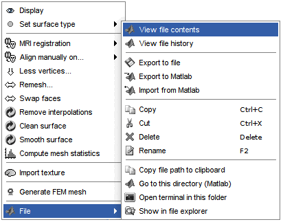
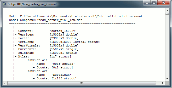
View file contents: Display all the fields in the Matlab .mat file.
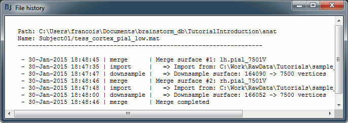
View file history: Review the History field in the file, that records all the operations that were performed on the file since if was imported in Brainstorm.
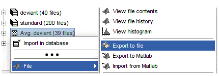
Export to file: Export in one of the supported mesh file format.
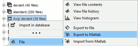
Export to Matlab: Load the contents of the .mat file in the Matlab base workspace. It is then accessible from the Matlab command window.
Import from Matlab: Replace the selected file with the content of a variable from the Matlab base workspace. Useful to save back in the database a structure that was exported and modified manually with the Matlab command window.
Copy / Cut / Paste: Allow you to copy/move files in the database explorer. Keyboard shortcuts for these menus are the standard Windows shortcuts (Ctrl+C, Ctrl+X, Ctrl+V). The database explorer also supports drag-and-drop operations for moving files between different folders.
Delete: Delete a file. Keyboard shortcuts: Delete key.
Rename: Change the Comment field in the file. It "renames" the file in the database explorer, but does not change the actual file name on the hard drive. Keyboard shortcut: F2
Copy file path to clipboard: Copies the full file name into the system clipboard, so that you can paste it in any other window (Ctrl+V or Paste menu)
Go to this directory (Matlab): Change the current Matlab path, so that you can access the file from the Matlab Command window or the Matlab Current directory window
Show in file explorer: Open a file explorer window in this directory.
Open terminal in this folder: Start a system console in the file directory (Linux and MacOS only).
What are all these other files ?
If you look in brainstorm_db/TutorialIntroduction with the file explorer of your operating system, you'll find many other directories and files that are not visible in the database explorer.
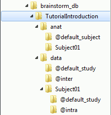
The protocol TutorialIntroduction is divided in Anatomy and Datasets directories:
Each subject in anat is described by an extra file: brainstormsubject.mat
Each folder in data is described by an extra file: brainstormstudy.mat
anat/@default_subject: Contains the files of the default anatomy (Default anatomy)
data/@default_study: Files shared between different subjects (Global common files)
data/@inter: Results of inter-subject analysis
data/Subject01/@default_study: Files shared between different folders in Subject01
data/Subject01/@intra: Results of intra-subject analysis (across different folders)
On the hard drive: MRI
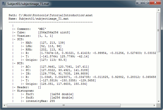
Right-click on the MRI > File > View file contents:
Structure of the MRI files: subjectimage_*.mat
Comment: String displayed in the database explorer to represent the file.
Cube: [Nsagittal x Ncoronal x Naxial] full MRI volume. Cube(1,1,1) is in the left, posterior, inferior corner.
Voxsize: Size of one voxel in millimeters (sagittal, coronal, axial).
SCS: Defines the Subject Coordinate System. Points below are in MRI RAS coordinate (in millimeters, i.e., voxel_number * voxel_size) coordinates. In Brainstorm voxel numbers are 1-indexed.
NAS: (x,y,z) coordinates of the nasion fiducial.
LPA: (x,y,z) coordinates of the left ear fiducial.
RPA: (x,y,z) coordinates of the right ear fiducial.
R: [3x3] rotation matrix from MRI coordinates to SCS coordinates.
T: [3x1] translation matrix from MRI coordinates to SCS coordinates.
Origin: MRI coordinates of the point with SCS coordinates (0,0,0).
NCS: Defines the MNI coordinate system, either with a linear or a non-linear transformation.
AC: (x,y,z) coordinates of the Anterior Commissure.
PC: (x,y,z) coordinates of the Posterior Commissure.
IH: (x,y,z) coordinates of an Inter-Hemisperic point.
- (Linear transformation)
R: [3x3] rotation matrix from MRI coordinates to MNI coordinates.
T: [3x1] translation matrix from MRI coordinates to MNI coordinates.
- (Non-linear transformation)
iy: 3D floating point matrix: Inverse MNI deformation field, as in SPM naming conventions. Same size as the Cube matrix, it gives for each voxel its coordinates in the MNI space, and is therefore used to convert from MRI coordinates to MNI coordinates.
y: 3D floating point matrix: Forward MNI deformation field, as in SPM naming conventions. For some MNI coordinates, it gives their coorrespondance in the original MRI space. To be interpreted, it has to be used with the matrix y_vox2ras.
y_vox2ras: [4x4 double], transformation matrix that converts from voxel coordinates of the y volume to MNI coordinates.
y_method: Algorithm used for computing the normalization ('segment'=SPM12 Segment)
Origin: MRI coordinates of the point with NCS coordinates (0,0,0).
Header: Header from the original file format (.nii, .mgz, ...)
Histogram: Result of the internal analysis of the MRI histogram, mainly to detect background level.
InitTransf: [Ntransform x 2] cell-matrix: Transformations that are applied to the MRI before importing the surfaces. Example: {'vox2ras', [4x4 double]}
Labels: [Nlabels x 3] cell-matrix: For anatomical parcellations, this field contains the names and RGB colors associated with each integer label in the volume. Example:
{0, 'Background', [0 0 0]}
{1, 'Precentral L', [203 142 203]}History: List of operations performed on this file (menu File > View file history).
Useful functions
/toolbox/io/in_mri_bst(MriFile): Read a Brainstorm MRI file and compute the missing fields.
/toolbox/io/in_mri(MriFile, FileFormat=[]): Read a MRI file (format is auto-detected).
/toolbox/io/in_mri_*.m: Low-level functions for reading all the file formats.
/toolbox/anatomy/mri_*.m: Routines for manipulating MRI volumes.
/toolbox/gui/view_mri(MriFile, ...): Display an imported MRI in the MRI viewer.
/toolbox/gui/view_mri_3d(MriFile, ...): Display an imported MRI in a 3D figure.
On the hard drive: Surface
Right-click on any cortex surface > File > View file contents:
Structure of the surface files: tess_*.mat
Atlas: Array of structures, each entry is one menu in the drop-down list in the Scout tab.
Name: Label of the atlas (reserved names: "User scouts", "Structures", "Source model")
Scouts: List of regions of interest in this atlas, see the Scout tutorial.
Comment: String displayed in the database explorer to represent the file.
Curvature: [Nvertices x 1], curvature value at each point.
Faces: [Nfaces x 3], triangles constituting the surface mesh.
History: List of operations performed on this file (menu File > View file history).
iAtlas: Index of the atlas that is currently selected for this surface.
Reg: Structure with registration information, used to interpolate the subject's maps on a template.
Sphere.Vertices: Location of the surface vertices on the FreeSurfer registered spheres.
Square.Vertices: Location of the surface vertices in the BrainSuite atlas.
AtlasSquare.Vertices: Corresponding vertices in the high-resolution BrainSuite atlas.
SulciMap: [Nvertices x 1], binary mask marking the botton of the sulci (1=displayed as darker).
tess2mri_interp: [Nvoxels x Nvertices] sparse interpolation matrix MRI<=>surface.
VertConn: [Nvertices x Nvertices] Sparse adjacency matrix, VertConn(i,j)=1 if i and j are neighbors.
Vertices: [Nvertices x 3], coordinates (x,y,z) of all the points of the surface, in SCS coordinates.
VertNormals: [Nvertices x 3], direction (x,y,z) of the normal to the surface at each vertex.
Useful functions
/toolbox/io/in_tess_bst(SurfaceFile): Read a Brainstorm surface file and compute the missing fields.
/toolbox/io/in_tess(TessFile, FileFormat=[], sMri=[]): Read a surface file (format is auto-detected).
/toolbox/io/in_tess_*.m: Low-level functions for reading all the file formats.
/toolbox/anatomy/tess_*.m: Routines for manipulating surfaces.
/toolbox/gui/view_surface(SurfaceFile, ...): Display an imported surface in a 3D figure.
/toolbox/gui/view_surface_data(SurfaceFile, OverlayFile, ...): Display a surface with a source map.
/toolbox/gui/view_surface_matrix(Vertices, Faces, ...): Display a mesh in a 3D figure.
Tutorial 4: Channel file / MEG-MRI coregistration
Authors: Francois Tadel, Elizabeth Bock, Sylvain Baillet
The anatomy of your subject is ready. Before we can start looking at the MEG/EEG recordings, we need to make sure that the sensors (electrodes, magnetometers or gradiometers) are properly aligned with the MRI and the surfaces of the subject.
In this tutorial, we will start with a detailed description of the experiment and the files that were recorded, then we will link the original CTF files to the database in order to get access to the sensors positions, and finally we will explore the various options for aligning these sensors on the head of the subject.
Contents
License
This dataset (MEG and MRI data) was collected by the MEG Unit Lab, McConnell Brain Imaging Center, Montreal Neurological Institute, McGill University, Canada. The original purpose was to serve as a tutorial data example for the Brainstorm software project. It is presently released in the Public Domain, and is not subject to copyright in any jurisdiction.
We would appreciate though that you reference this dataset in your publications: please acknowledge its authors (Elizabeth Bock, Peter Donhauser, Francois Tadel and Sylvain Baillet) and cite the Brainstorm project seminal publication.
Presentation of the experiment
Experiment
- One subject, two acquisition runs of 6 minutes each.
- Subject stimulated binaurally with intra-aural earphones (air tubes+transducers), eyes opened and looking at a fixation cross on a screen.
- Each run contains:
- 200 regular beeps (440Hz).
- 40 easy deviant beeps (554.4Hz, 4 semitones higher).
- Random inter-stimulus interval: between 0.7s and 1.7s seconds, uniformly distributed.
- The subject presses a button when detecting a deviant with the right index finger.
- Auditory stimuli generated with the Matlab Psychophysics toolbox.
The specifications of this dataset were discussed initially on the FieldTrip bug tracker:
http://bugzilla.fieldtriptoolbox.org/show_bug.cgi?id=2300.
MEG acquisition
Acquisition at 2400Hz, with a CTF 275 system, subject in sitting position
- Recorded at the Montreal Neurological Institute in December 2013
- Anti-aliasing low-pass filter at 600Hz, files saved with the 3rd order gradient
Downsampled at a lower sampling rate: from 2400Hz to 600Hz: The only purpose for this resampling is to make the introduction tutorials easier to follow the on a regular computer.
- Recorded channels (340):
- 1 Stim channel indicating the presentation times of the audio stimuli: UPPT001 (#1)
- 1 Audio signal sent to the subject: UADC001 (#316)
- 1 Response channel recordings the finger taps in response to the deviants: UDIO001 (#2)
- 26 MEG reference sensors (#5-#30)
- 274 MEG axial gradiometers (#31-#304)
- 2 EEG electrodes: Cz, Pz (#305 and #306)
- 1 ECG bipolar (#307)
- 2 EOG bipolar (vertical #308, horizontal #309)
- 12 Head tracking channels: Nasion XYZ, Left XYZ, Right XYZ, Error N/L/R (#317-#328)
- 20 Unused channels (#3, #4, #310-#315, #329-340)
- 3 datasets:
S01_AEF_20131218_01_600Hz.ds: Run #1, 360s, 200 standard + 40 deviants
S01_AEF_20131218_02_600Hz.ds: Run #2, 360s, 200 standard + 40 deviants
S01_Noise_20131218_02_600Hz.ds: Empty room recordings, 30s long
- Average reaction times for the button press after a deviant tone:
Run #1: 515ms +/- 108ms
Run #2: 596ms +/- 134ms
Head shape and fiducial points
3D digitization using a Polhemus Fastrak device driven by Brainstorm (S01_20131218_01.pos)
More information: Digitize EEG electrodes and head shape
- The output file is copied to each .ds folder and contains the following entries:
- The position of the center of CTF coils.
The position of the anatomical references we use in Brainstorm:
Nasion and connections tragus/helix, as illustrated here.- Around 150 head points distributed on the hard parts of the head (no soft tissues).
Link the raw files to the database
Switch to the "functional data" view.
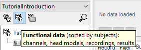
Right-click on the subject folder > Review raw file
Select the file format: "MEG/EEG: CTF (*.ds...)"
Select all the .ds folders in: sample_introduction/data
- In the CTF file format, each session of recordings is saved in a folder with the extension "ds". The different types of information collected during each session are saved as different files in this folder (event markers, sensor definitions, bad segments, MEG recordings).

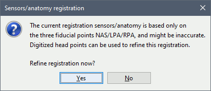
Refine registration now? YES
This operation is detailed in the next section.
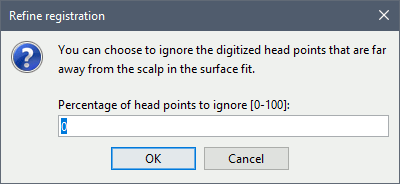
Percentage of head points to ignore: 0
If you have some points that were not digitized correctly and that appear far from the head surface, you should increase this value in order to exclude them from the fit.
Automatic registration
The registration between the MRI and the MEG (or EEG) is done in two steps. We start with a first approximation based on three reference points, then we refine it with the full head shape of the subject.
Step 1: Fiducials
The initial registration is based on the three fiducial points that define the Subject Coordinate System (SCS): nasion, left ear, right ear. You have marked these three points in the MRI viewer in the previous tutorial.
These same three points have also been marked before the acquisition of the MEG recordings. The person who recorded this subject digitized their positions with a tracking device (such as a Polhemus FastTrak or Patriot). The position of these points are saved in the dataset.
- When we bring the MEG recordings into the Brainstorm database, we align them on the MRI using these fiducial points: we match the NAS/LPA/RPA points digitized with the ones we located in the MRI Viewer.
This registration method gives approximate results. It can be good enough in some cases, but not always because of the imprecision of the measures. The tracking system is not always very precise, the points are not always easy to identify on the MRI slides, and the very definition of these points does not offer a millimeter precision. All this combined, it is easy to end with an registration error of 1cm or more.
The quality of the source analysis we will perform later is highly dependent on the quality of the registration between the sensors and the anatomy. If we start with a 1cm error, this error will be propagated everywhere in the analysis.
Step 2: Head shape
To improve this registration, we recommend our users to always digitize additional points on the head of the subjects: around 100 points uniformly distributed on the hard parts of the head (skull from nasion to inion, eyebrows, ear contour, nose crest). Avoid marking points on the softer parts (cheeks or neck) because they may have a different shape when the subject is seated on the Polhemus chair or lying down in the MRI. More information on digitizing head points.
- We have two versions of the full head shape of the subject: one coming from the MRI (the head surface, represented in grey in the figures below) and one coming from the Polhemus digitizer at the time of the MEG/EEG acquisition (represented as green dots).
The algorithm that is executed when you chose the option "Refine registration with head points" is an iterative algorithm that tries to find a better fit between the two head shapes (grey surface and green dots), to improve the intial NAS/LPA/RPA registration. This technique usually improves significantly the registration between the MRI and the MEG/EEG sensors.
- Tolerance: If you enter a percentage of head points to ignore superior to zero, the fit is performed once with all the points, then the head points the most distant to the cortex are removed, and the fit is executed a second time with the head points that are left.
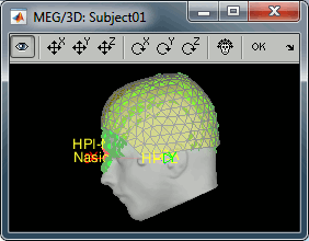
- The two pictures below represent the registration before and after this automatic head shape registration (left=step 1, right=step 2). The yellow surface represents the MEG helmet: the solid plastic surface in which the subject places his/her head. If you ever see the grey head surface intersecting this yellow helmet surface, there is obviously something wrong with the registration.
At the end of the import process, you can close the figure that shows the final registration.
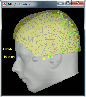
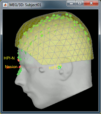
A window reporting the distance between the scalp and the head points is displayed. You can use these values as references for estimating whether you can trust the automatic registration or not. Defining whether the distances are correct or abnormal depend on your digitization setup.

Defaced volumes
When processing your own datasets, if your MRI images are defaced, you might need to proceed in a slightly different way. The de-identification procedures remove the nose and other facial features from the MRI. If your digitized head shape includes points on the missing parts of the head, this may cause an important bias in automatic registration. In this case it is advised to remove the head points below the nasion before proceeding to the automatic registration, as illustrated in this tutorial.
New files and folders
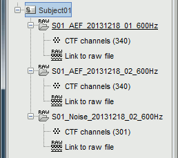
Many new files are now visible in the database explorer:
- Three folders representing the three MEG datasets that we linked to the database. Note the tag "raw" in the icon of the folders, this means that the files are considered as new continuous files.
S01_AEF_20131218_01_600Hz: Subject01, Auditory Evoked Field, 18-Dec-2013, run #01
S01_AEF_20131218_02_600Hz: Subject01, Auditory Evoked Field, 18-Dec-2013, run #02
S01_Noise_20131218_02_600Hz: Subject01, Noise recordings (no subject in the MEG)
- All three have been downsampled from 2400Hz to 600Hz.
Each of these new folders show two elements:
Channel file: Defines the types and names of channels that were recorded, the position of the sensors, the head shape and other various details. This information has been read from the MEG datasets and saved as a new file in the database. The total number of data channels recorded in the file is indicated between parenthesis (340).
Link to raw file: Link to the original file that you imported. All the relevant meta-data was read from the MEG dataset and copied inside the link itself (sampling rate, number of samples, event markers and other details about the acquisition session). But no MEG/EEG recordings were read or copied to the database. If we open this file, the values are read directly from the original files in the .ds folder.
Review vs Import
When trying to bring external data into the Brainstorm environment, a common source of confusion is the difference between the two popup menus Review and Import:
Review raw file: Allows you to create a link to your original continuous data file. It reads the header and sensor information from the file but does not copy the recordings in the database. Most of the artifact cleaning should be done directly using these links.
Import MEG/EEG: Extract segments of recordings (epochs) from an external file and saves copies of them in the Brainstorm database. You should not be using this menu until you have fully pre-processed your recordings, or if you are importing files that are already epoched or averaged.
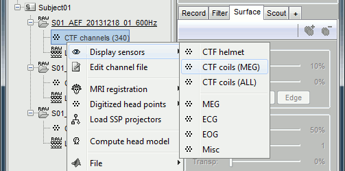
Display the sensors
Right-click on the CTF channels file and try all the display menus:
CTF Helmet: Shows a surface that represents the inner surface of the MEG helmet.
CTF coils (MEG): Display the MEG head coils of this CTF system: they are all axial gradiometers, only the coils close to the head are represented. The small squares do not represent the real shape of the sensors (the CTF coils are circular loops) but an approximation made in the forward model computation.
CTF coils (ALL): Display all the MEG sensors, including the reference magnetometers and gradiometers. The orientation of the coils is represented with a red segment.
MEG: MEG sensors are represented as small white dots and can be selected by clicking on them.
ECG / EOG: Ignore these menus, we do not have proper positions for these electrodes.
Misc: Shows the approximate positions of the EEG electrodes (Cz and Pz).
Use the [Close all] button to close all the figures when you are done.

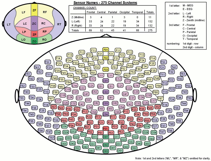
Sensor map
Here is a map with the full list of sensor names for this CTF system, it could be useful for navigating in the recordings. Click on the image for a larger version.
Manual registration
If the registration you get with the automatic alignment is incorrect, or if there was an issue when you digitized the position of the fiducials or the head shape, you may have to realign manually the sensors on the head. Right-click on the channel file > MRI Registration:
Check: Show all the possible information that may help to verify the registration.
Edit: Opens a window where you can move manually the MEG helmet relative to the head.
Read the tooltips of the buttons in the toolbar to see what is available, select an operation and then right-click+move up/down to apply it. From a scientific point of view this is not exactly a rigorous operation, but sometimes it is much better than using wrong default positions.
IMPORTANT: this refinement can only be used to better align the headshape with the digitized points - it cannot be used to correct for a subject who is poorly positioned in the helmet (i.e. you cannot move the helmet closer to the subjects head if they were not seated that way to begin with!)
Refine using head points: Runs the automatic registration described earlier.
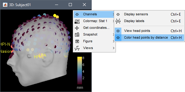
In the 3D views, the head points can be color-coded to represent the distance to the scalp. Right-click on the figure > Channels > Color head points by distance (shortcut CTRL+H). The colorbar indicates in millimeters the distance of each point to the scalp, as compute by bst_surfdist.m.
There is nothing to change here, but remember to always check the registration scalp/sensors.
Multiple runs and head positions
Between two acquisition runs the subject may move in the MEG helmet, the relative position of the MEG sensors with the head surface changes. At the beginning of each MEG run, the positions of the head localization coils are detected and used to update the position of the MEG sensors.
- The two AEF runs 01 and 02 were acquired successively. The position of the subject's head in the MEG helmet was estimated twice, once at the beginning of each run.
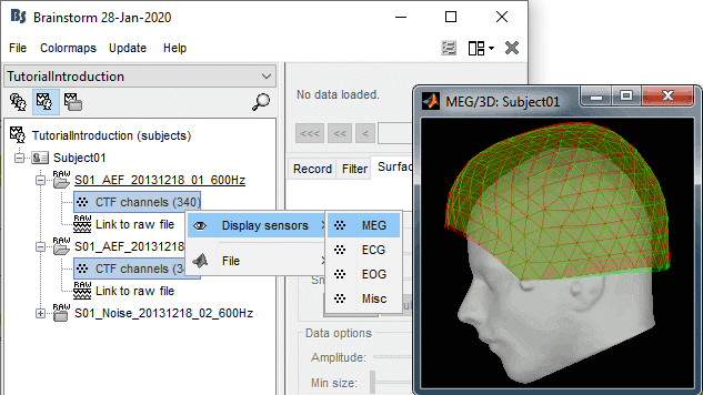
To evaluate visually the displacement between the two runs, select at the same time all the channel files you want to compare (the ones for run 01 and 02), right-click > Display sensors > MEG.

- Typically, we would like to group the trials coming from multiple acquisition runs. However, because of the subject's movements between runs, it is usually not possible to directly compare the MEG values between runs. The sensors may not capture the activity coming from the same regions of the brain.
- You have three options if you consider grouping information from multiple runs:
Method 1: Process all the runs separately and average between runs at the source level: The more accurate option, but requires more work, computation time and storage.
Method 2: Ignore movements between runs: This can be acceptable if the displacements are really minimal, less accurate but much faster to process and easier to manipulate.
Method 3: Co-register properly the runs using the process Standardize > Co-register MEG runs: Can be a good option for displacements under 2cm.
Warning: This method has not be been fully evaluated on our side, use at your own risk. Also, it does not work correctly if you have different SSP projectors calculated for multiple runs.
- In this tutorial, we will illustrate only method 1: runs are not co-registered.
Edit the channel file
Display a table with all the information about the individual channels. You can edit all the values.
Right-click on the channel of the first folder (AEF#01) > Edit channel file:

Index: Index of the channel in the data matrix. Can be edited to reorder the channels.
Name: Name that was given to the channel by the acquisition device.
Type: Type of information recordeded (MEG, EEG, EOG, ECG, EMG, Stim, Other, "Delete", etc)
- You may have to change the Type for some channels. For instance if an EOG channel was saved as a regular EEG channel, you have to change its type to prevent it from being used in the source estimation.
- To delete a channel from this file: select "(Delete)" in the type column.
Group: Used to define sub-group of channels of the same type.
- SEEG/ECOG: Each group of contacts can represent a depth electrode or a grid, and it can be plotted separately. A separate average reference montage is calculated for each group.
- MEG/EEG: Not used.
Comment: Additional description of the channel.
- MEG sensors: Do not edit this information if it is not empty.
Loc: Position of the sensor (x,y,z) in SCS coordinates. Do not modify this from the interface.
One column per coil and per integration point (information useful for the forward modeling).Orient: Orientation of the MEG coils (x,y,z) in SCS coordinates). One column per Loc column.
Weight: When there is more than one coil or integration point, the Weight field indicates the multiplication factor to apply to each of these points.
- To edit the type or the comment for multiple sensors at once, select them all then right-click.
- Close this figure, do not save the modifications if you made any.
On the hard drive
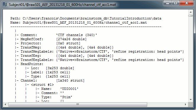
Some other fields are present in the channel file that cannot be accessed with the Channel editor window. You can explore these other fields with the File menu, selecting View file contents or Export to Matlab, as presented in the previous tutorial.
Structure of the channel files: channel_*.mat
Comment : String that is displayed in the Brainstorm database explorer.
MegRefCoef: Noise compensation matrix for CTF and 4D MEG recordings, based on some other sensors that are located far away from the head.
Projector: SSP/ICA projectors used for artifact cleaning purposes. See the SSP tutorial.
TransfMeg / TransfMegLabel: Transformations that were applied to the positions of the MEG sensors to bring them in the Brainstorm coordinate system.
TransfEeg / TransfEegLabel: Same for the position of the EEG electrodes.
HeadPoints: Extra head points that were digitized with a tracking system.
Channel: An array that defines each channel individually (see previous section).
Clusters: An array of structures that defines channels of clusters, with the following fields:
Sensors: Cell-array of channel names
Label: String, name of the cluster
Color: RGB values between 0 and 1 [R,G,B]
Function: String, cluster function name (deault: 'Mean')
History: Describes all the operations that were performed with Brainstorm on this file. To get a better view of this piece of information, use the menu File > View file history.
IntraElectrodes: Definition of iEEG devices, documented in the SEEG tutorial.
Useful functions
/toolbox/io/import_channel.m: Read a channel file and save it in the database.
/toolbox/io/in_channel_*.m: Low-level functions for reading all the file formats.
/toolbox/io/in_bst_channel.m: Read a channel file saved in the database.
/toolbox/sensors/channel_*.m: Routines for manipulating channel files.
/toolbox/gui/view_channels(ChannelFile, Modality, ...): Display the sensors in a 3D figure.
Additional documentation
Forum: Import the position of SEEG/ECOG contacts: Post #2206, Post #1958, Post #2357
Tutorial 5: Review continuous recordings
Authors: Francois Tadel, Elizabeth Bock, Raymundo Cassani, John C Mosher, Sylvain Baillet
Contents
Open the recordings
Let's look at the first file in the list: AEF#01.
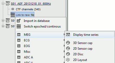
Right-click on the Link to raw file. Below the first to menus, you have the list of channel types:
MEG: 274 axial gradiometers
ECG: 1 electrocadiogram, bipolar electrode across the chest
EOG: 2 electrooculograms (vertical and horizontal)
Misc: EEG electrodes Cz and Pz
ADC A: Unused
ADC V: Auditory signal sent to the subject
DAC: Unused
FitErr: Fitting error when trying to localize the three head localization coils (NAS, LPA, RPA)
HLU: Head Localizing Unit, displacements in the three directions (x,y,z) for the three coils
MEG REF: 26 reference sensors used for removing the environmental noise
Other: Unused
Stim: Stimulation channel, records the stim triggers generated by the Psychophysics toolbox and other input channels, such as button presses generated by the subject
SysClock: System clock, unused
Select > MEG > Display time series (or double-click on the file).
It will open a new figure and enable many controls in the Brainstorm window.
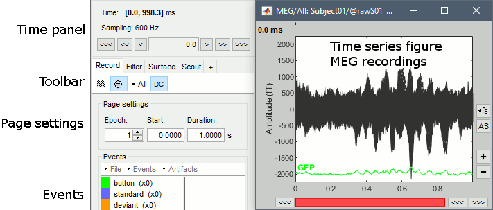
Navigate in time
The files we have imported here are shown the way they have been saved by the CTF MEG system: as contiguous epochs of 1 second each. These epochs are not related with the stimulus triggers or the subject's responses, they are just a way of saving the files. We will first explore the recordings in this epoched mode before switching to the continuous mode.
From the time series figure
Click: Click on the white or grey parts of figure to move the time cursor (red vertical line).
If you click on the signals, it selects the corresponding channels. Click again to unselect.Shortcuts: See the tooltips in the time panel for important keyboard shortcuts:
Left arrow, right arrow, page up, page down, F3, Shift+F3, etc...Bottom bar: The red square in the bottom bar represents the portion of the file that is currently displayed from the current file or epoch. Right now we show all the epoch #1. This will be more useful in the continuous mode.
Zoom: Scroll to zoom horizontally around the time cursor (mouse wheel or two-finger up/down).
[<<<] and [>>>]: Previous/next epoch or page
From the time panel
Time: [0, 998]ms is the time segment over which the first epoch is defined.
Sampling: We downsampled these files to 600Hz for easier processing in the tutorials.
Text box: Current time, can be edited manually.
[<] and [>]: Previous/next time sample - Read the tooltip for details and shortcuts
[<<] and [>>]: Previous/next time sample (x10) - Read the tooltip for details and shortcuts
[<<<] and [>>>]: Previous/next epoch or page - Read the tooltip for details and shortcuts
From the page settings
Epoch: Selects the current time block that is displayed in the time series figure.
Start: Starting point of the time segment displayed in the figure. Useful in continuous mode only.
Duration: Length of this time segment. Useful in continuous mode only.
Time selection
- In the time series figure, click and drag your mouse for selecting a time segment.
- At the bottom of the figure, you will see the duration of the selected block, and min/max values.
- Useful for quickly estimating the latencies between two events, or the period of an oscillation.
To zoom into the selection: Shift+left click, middle click, or right-click > Time selection > Zoom into.
Click anywhere on the figure to cancel this time selection.

Epoched vs. continuous
- The CTF MEG system can save two types of files: epoched (.ds) or continuous (_AUX.ds).
- Here we have an intermediate storage type: continuous recordings saved in "epoched" files. The files are saved as small blocks of recordings of a constant time length (1 second in this case). All these time blocks are contiguous, there is no gap between them.
- Brainstorm can consider this file either as a continuous or an epoched file. By default it imports the regular .ds folders as epoched, but we need to change this manually.
Right-click on the "Link to raw file" for AEF#01 > Switch epoched/continuous
You should get a message: "File converted to: continuous".Double-click on the "Link to raw file" again. Now you can navigate in the file without interruptions. The box "Epoch" is disabled and all the events in the file are displayed at once.
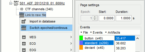
With the red square at the bottom of the figure, you can navigate in time (click in the middle and drag with the mouse) or change the size of the current page (click on the left or right edge of the red square and move your mouse).

Increase the duration of the displayed window to 3 seconds (Page settings > Duration).
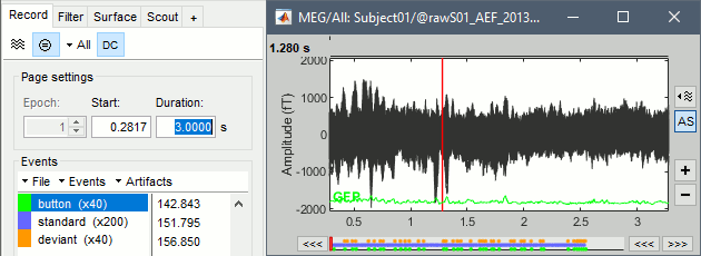
- Close the figure.
- Repeat this operation with the other files to convert them all to a continuous mode.
AEF#02 > Switch epoched/continuous
Noise > Switch epoched/continuous
Display mode: Butterfly/Column
- Close all the figures.
- Double-click on the AEF#01 Link to raw file to open the MEG recordings.
- What we see are all the traces of the 274 sensors overlaid on top of each other.
Click on the "Display mode" button in the toolbar of the Record tab.

All the signals are now displayed, one below the other, but because we have 274 MEG channels the figure is still unreadable. We need to select only a subset of these sensors.
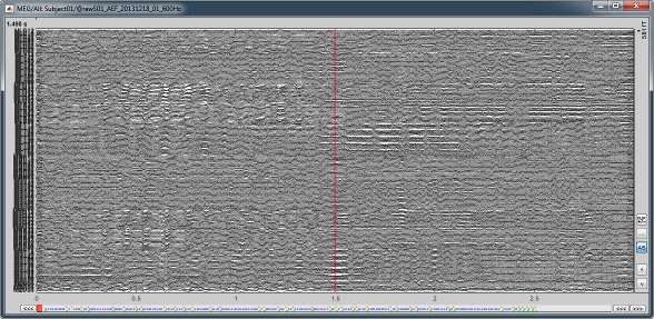
Montage selection
- You can use the montage menu to select a group of sensors. This menu is accessible in two ways:
Record toolbar > Drop-down menu.
Figure popup menu > Right-click on the figure > Montage
Pre-defined groups of channels are available for some common MEG and EEG systems.
Notice the keyboard shortcut on the right for All channels (Shift+A). You can define your own (Shift+B, C...) if you go to Edit montages.You can also use this menu to create your own sensor selections or more complex montages.
A separate tutorial is dedicated to the montage editor.Select the group: CTF LT (Left Temporal).
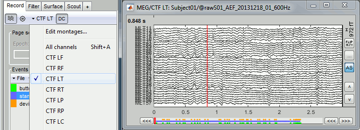
More information about the Montage editor.
Channel selection
If you click on the white or grey areas of the figure, it changes the current time.
If you click on the lines representing the recorded signals instead, it selects the corresponding channels.
- When some channels are selected, an additional menu "Channels" is visible in the figure popup.
- Select "View selected" or press [Enter] to open the selected channels in a separate window.
The management of the bad channels will be introduced in a separate tutorial.
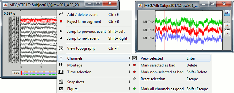
Amplitude scale
A variety of display options allows you to adjust the amplitude scale for the recordings (vertical axis). Most of these options are available in the right part of the time series figure, some are repeated in the Record tab of the Brainstorm window.
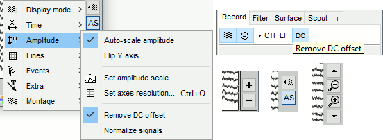
Increase/decrease gain: Buttons [+] and [-] on the right side of the figure. The shortcuts for these buttons are indicated in the tooltips (leave the mouse for a short while over a button): right-click and move your mouse, hold the Shift key and scroll, or use the keys "+" and "-".
Auto-scale amplitude: Button [AS] in the figure.
Selected: the vertical scale is adapted to the new maximum amplitude when you scroll in the file.
Not selected: The vertical scale is fixed, scrolling in the file does not affect the axis resolution.Flip Y axis: Exchange the direction of the Y axis, to have the peaks of negative values pointing up. Useful mostly for clinical EEG.
Set amplitude scale: Opens a window to enter the amplitude scale manually. The value corresponds to the space between two horizontal lines in this figure.
Set axis resolution: See section "Time and amplitude resolution" below.
Remove DC offset: Button [DC] in the Record tab. When selected, the average value over the entire current time window is subtracted from each channel. This means that if you change the length of the time window, the value that is removed from each channel may change. Always keep this option selected for unprocessed MEG recordings, unless you use a high-pass filter.
Normalize signals: Divide each signal by its maximal amplitude in the displayed time window. The signals displayed with this normalization are unitless.
Apply CTF compensation: Button [CTF] in the Record tab. Enable/disable the CTF noise correction based on the reference sensors, when it is not already applied in the file. In the current file, the CTF 3rd order gradient compensation is already applied, therefore this option is not available.
Vertical zoom: Use the zoom/scrolll buttons on the right of the figure or your mouse (CTRL+Mouse wheel to zoom, middle-click+move to scroll) in order to look at specific channels without having to change the montage.

Uniform amplitude scales: Force all the time series figures to use the same amplitude scale. Option available in the Record tab with the button
 or from the figure options menu when at least two time series figures are visible. More details.
Time and amplitude resolution
In the Brainstorm interface, the axis resolution is usually set implicitly: you can set the size of the window, the duration or recordings reviewed at once and the maximum amplitude to show in the figure. These parameters are convenient to explore the recordings interactively but don't allow us to have reproducible displays with constant time and amplitude resolutions.
However, some applications are very sensitive to the horizontal and vertical scaling, such as the visual detection of epileptic spikes. The shapes of traces the epileptologists try to identify are altered by the axes resolution. This is detailed in the tutorial EEG and Epilepsy.
For this reason, we also added an option to set the figure resolution explicitly. The distance unit on a screen is the pixel, we can set precisely how much time is represented by one pixel horizontally and how much amplitude is represented by one pixel vertically.
Display menu in the right part of the figure > Amplitude > Set axis resolution (shortcut: CTRL+O)
Note that this interface does not store the input values, it just modifies the other parameters (figure size, time window, max amplitude) to fit the resolution objectives. If you modify these parameters after setting the resolution (resize the figure, leave the button [AS] selected and scroll in time, etc) the resolution is lost, you have to set it again manually.
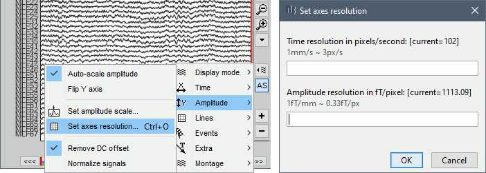
Absolute and relative time
Some recordings file formats include in their meta-data a real-world timestamp. When this timestamp is available, it allows to display signals in either absolute time (HH:MM:SS) or relative time (usually 0 s indicate the beginning of the file). To change the time format for the x-axis, use the go to the Display menu in the right part of the figure > Time > Display time as {absolute | relative} time (shortcut: CTRL+X). In addition, you can get the timestamp for the current time (vertical red cursor) by doing right-click anywhere in the figure.

Filters for visualization
With the Filter tab, you can apply a band-pass filter to the recordings, or remove a set of specific frequencies (example: the 50Hz or 60Hz power lines contamination and their harmonics). The filters are applied only to the time window that is currently loaded. If the segment is too short for the required filters, the results might be inaccurate.
These visualization filters provide a quick estimate for visualization only, the results are not saved anywhere. To filter properly the continuous files, please use the Process1 tab (see tutorial #10).
The option "Filter all results" is not useful for now, it will be described later.
After testing the high-pass, low-pass and notch filters, uncheck them. Otherwise you may forget about them, they would stay on until you restart Brainstorm. Note that as long as there are visualization filters applied, the title of the Filter tab remains red.
Mouse and keyboard shortcuts
Keyboard shortcuts
Left / right arrows:
- Change current time, sample by sample
+Control key: Jump to previous/next epoch or page (same as [<<<] and [>>>])
+Shift key: Jump to previous/next event (you need to have one event selected)
MacOS: These shortcuts are different, please read the tooltips for [>], [>>] and [>>>]
Page-up / page-down:
- Change current time, 10 samples at a time
+Control key: Jump to the next/previous epoch or page, 10x faster
F3/Shift+F3: Jump to the next/previous epoch or page (10% overlap between 2 pages)
F4/Shift+F4: Jump to the next/previous half-page (50% overlap)
F6/Shift+F6: Jump to the next/previous page with no overlap (0% overlap)
Plus / minus: Adjust the vertical scale of the time series
Shift + Letter: Changes the montage
Control + B: Mark selected time segment as bad
Control + D: Dock figure
E: Add / delete event marker
Control + E: Add / delete event marker for the selected channels
Control + F: Open a copy of the figure, not managed by the Brainstorm window manager
Control + H: Hide/show selected event group
Control + I: Save figure as image
Control + J: Open a copy of the figure as an image
Control + O: Set axes resolution
Control + L: Change display mode of events (dots, lines or hidden)
Control + J: Open a screen capture of the figure
Control + T: Open a 2D topography window at the current time
Enter: Display the selected channels in a separate figure
Escape: Unselect all the selected channels
Delete: Mark the selected channels as bad
1 2 3 4 5 6 7 8 9: User-defined shortcuts for new events (tutorial #7)
Mouse shortcuts
Click on a channel: Select the channel
Click: Change current time
Shift + click: Force the selection of the current time (even when clicking on a channel)
Click + move: Select time range
Right-click: Display popup menu
Right-click + move: Adjust the vertical scale of the time series
Scroll: Zoom around current time
Shift + scroll: Adjust the vertical scale of the time series
Control + scroll: Zoom vertically
Central click + move: Move in a zoomed figure
Double click: Restore initial zoom settings (or edit the notes associated to the clicked event)
Tutorial 6: Multiple windows
Authors: Francois Tadel
Contents
General organization
This tutorial is a parenthesis to explain how the figures are positioned on the screen and how you can organize your workspace more efficiently. One interesting feature of the Brainstorm interface is the ability to open easily multiple views or multiple datasets simultaneously.
The buttons in the menu "Window layout options" can help you organize all the opened figures in an efficient way. There are four options for the automatic placement of the figures on the screen and you have the possibility to save your own specific working environment.
Remember that the Brainstorm window is designed to remain on one side of the screen. All the space of the desktop that is not covered by this window will be used for opening other figures. This available space is designated in the menus below as "Full area". Do not try to maximize the Brainstorm window, or the automatic management of the data figures might not work correctly.
Automatic figure positioning
Layout options: Defines how the figures are positioned on the screen
Tiled: All the figures have similar sizes.
Weighted: Some figures containing more information are given more space on the screen. This mode is mostly useful when reviewing continuous recordings.
Full area: Each figure takes all the space available for figures.
None: The new figures are displayed at the default Matlab position, always at the same place, and never re-organized after. Selecting this option can be useful if the auto-arrangement does not work well on your system or if you want to organize your windows by yourself. It is also automatically selected when using "user setups" (see below).
One screen / two screens: If you have multiple monitors, Brainstorm can try to place the database window on one screen and all the other figures on the other screen. If you force Brainstorm to use only one screen, all the figures should stay on the same screen.
Full screen: If selected, the figures are set to their maximum size, covering the Brainstorm window
Show all figures: If you have many figures hidden by some other fullscreen window (Matlab, Firefox to read this tutorial, etc), you don't have click on all of them in the taskbar to get them back. Just make the Brainstorm window visible and click on this button, it would bring all the figures back (not working on some Linux window managers).
User setups: You can save a combination of figures currently opened on your desktop and re-use it later on a different dataset. It can be very useful for reviewing long continuous files.
Close all figures: Last button in the toolbar. Close everything and free the allocated memory.
Example
Double-click on AEF#01 Link to raw file to open the MEG sensors.
Open the EOG signals for the same file: Right-click on the file > EOG > Display time series.
Open a 2D topography for the MEG sensors: Right-click on the file > MEG > 2D sensor cap.
This view represents the values of the all the MEG sensors at the current time point. This type of figures will be described in another tutorial.Cycle through the options: Tiled, Weighted, Full area.
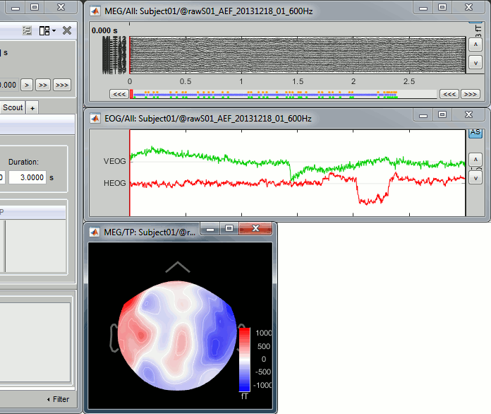
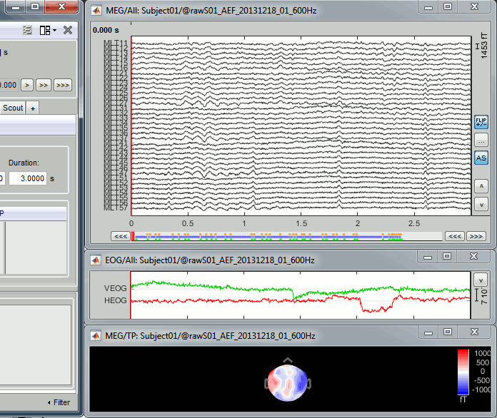
Select the option None, close all the figures (using the [Close all] button), and re-open them.
Notice that now the position of the figures is not managed by Brainstorm anymore.Select again Weighted: the figures are automatically re-arranged again.
Test the option Full screen.
If you have two screens connected, you can try the options One screen / Two screens.
Multiple views of the same data
- Keep all the existing figures: MEG, EOG, 2D topography.
- Open another time series view of the same file, same MEG sensors.
- Note that if you double-click again on the file, it just selects the existing figure.
To force opening another view: Right-click on the file > MEG > Display time series.
- Only the first view that was open on this file shows the events bar and the time navigation bar at the bottom of the figure. If you want the two MEG figures displayed in the exact same way, you can close everything, then start by opening the EOG view, then two MEG views.
- Re-arrange the figures in a nicer way.
Select montage "CTF LT" for one figure, and montage "CTF RF" for the other.
- You can change individually the display properties of each figure.
- When creating a new figure, it re-uses the last display properties that were used.
To change the properties of one figure, you have first to select this figure. Clicking on the title bar of the figure is not enough, you have to click inside the figure (this is due to some limitations of the Matlab figures implementation).
- When the new figure is selected, the controls in the Record tab are updated, and you can change the display properties for this figure.
There is currently a limitation relative to the continuous file viewer: it is not possible to review two continuous datasets at the same time. This is usually not a problem because we typically review the continuous files one after the other. It will be possible to open multiple data files after we import them in the database, this is what is really useful.
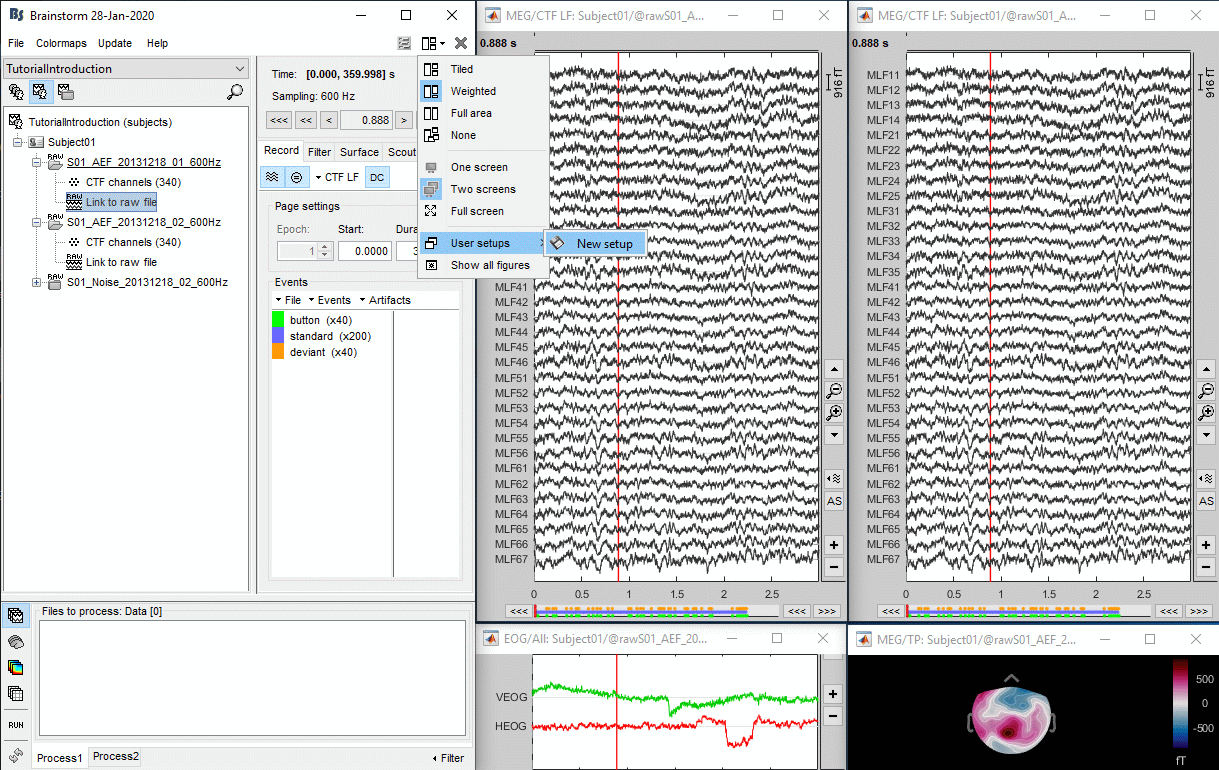
User setups
- Keep the four figures previously created (MEG LT, MEG RF, EOG, 2D sensor).
In the menu "Window layout options" > User setups > New setup > "Test".
- Close all the figures (using the Close all button).
- Double-click again on the Link to raw file to open MEG sensors.
In the menu "Window layout options" > User setups > Test.
It should restore your desktop exactly like it was when you saved it.Note that the layout None is now selected. Using custom window configurations disables the automatic arrangement of the windows on the screen.
- This feature is interesting for users who need to review numerous files everyday in a very specific way, for instance in the case of visual inspection of epilepsy recordings. It can save them a substantial amount of time to load their reviewing environment in just one click.
Uniform amplitude scales
Set the display mode "butterfly" for the two MEG time series figures:
Uncheck the first button in the Record tab.With the button Uniform amplitude scale
 , in the Record tab, you can change the way the amplitude of multiple time series figures is scaled.
 Selected: All the time series figures with similar units have the same y-axis scale, you can compare visually the amplitudes between two datasets.
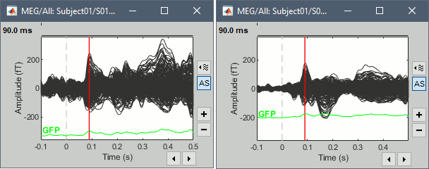
Not selected: Each figure is scaled independently to its own maximum amplitude.
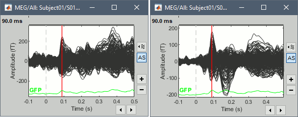
Graphic bugs
If you observe any graphic problem with these displays, there might be an issue with the OpenGL drivers. You may try the following options:
- Update the drivers for your graphics card.
- Upgrade your version of Matlab.
Run the compiled version of Brainstorm (see Installation).
Turn off the OpenGL hardware acceleration: Menu File > Edit preferences > Software or Disabled.
- Send a bug report to the Mathworks.
Tutorial 7: Event markers
Authors: Francois Tadel, Elizabeth Bock, John C Mosher, Raymundo Cassani
Contents
Lists of events
You probably noticed colored dots on top of the recordings in the MEG figure. They represent the event markers saved in this dataset. In this documentation, they can be called indifferently events, markers or triggers. Some are stimulus triggers that were generated by the stimulation computer (Psychtoolbox-3), others are the subject responses recorded from a button box. This tutorial shows how to manipulate these markers.
Open the MEG recordings for file AEF#01.
- Make sure it is configured as presented here: Montage "CTF LT", [DC] button selected, 3s pages.
- All the markers available in the file are listed in the Events section of the Record tab.
- On the left, you have the groups of events and the number of occurrence for each group:
200 standard audio stimulations
40 deviant audio stimulations
40 button responses: The subject presses a button with the right index finger when a deviant is presented. This is a very easy task so all the deviants are detected
- On the right, you have the list of the time instants at which the selected event occurs.
These two lists are interactive. If you click on an event group (left list), it shows the corresponding occurrences in the right list. If you click on one particular event in the right list, the file viewer jumps to it. It works the other way as well: if you click on a dot representing an event in the MEG figure, the corresponding event group and occurrence are selected in the Record tab.
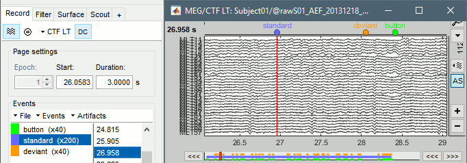
Adding events
The markers can represent either stimulation triggers or subject responses that were recorded during the acquisition. It can also be useful to add new markers during the analysis of the recordings, to identify events of interest that are not detected at the time of the recordings, such as artifacts (eye movements, heartbeats, subject movements) or specific patterns of brain activity (epileptic spikes).
Create a new group of events "Test" with the menu Events > Add group.
Click on this new category to select it. It contains no occurrences at the beginning (x0).

- Then place the time cursor (red vertical bar) where you want to add a new marker "Test".
- Add a few occurrences with any of the three methods:
In the Record tab: Select the menu Events > Add / delete event
In the time series figure: Right-click > Add / delete event
In the time series figure: Press key E
If the display is too dense, it can be difficult to set the current time instead of selecting a channel. Note that you can click outside of the white area to select the time (on top of the figure), or use the shortcut Shift+click.

- Remove all the event occurrences in "Test", but not the group itself. Use any of the three methods:
In the Record tab: Select one or more event occurrences, press the Delete key.
In the time series figure: Click on an event dot and right-click > Add / delete event.
In the time series figure: Click on an event dot and press key E.
Extended events
You can also use this interface to create events that have a temporal extension, i.e., that last for more than one time sample. This can be used to define bad segments in the recordings.
- In the time series window, select a time range (click + move).
Add an event: menus or key E.
The first occurrence you add in an event group defines its type: single time point (simple events), or time range (extended events). You cannot mix different types of events in a group. You get an error when you try to add a time segment in an event category that already contains a simple event.

Remove the event group "Test": Click on it in the list and press the Delete key.
Bad segments
It is very common to have portions of the recordings heavily contaminated by events coming from the subject (eye blinks, movements, heartbeats, teeth clenching) or from the environment (stimulation equipment, elevators, cars, trains, building vibrations...). Some of them are well defined and can be removed efficiently, some are too complex to be modeled efficiently. For this last category, it is usually safer to mark the noisy segments as bad, and ignore them for the rest of the analysis.
To mark a segment of recordings as bad, the procedure is the same as for defining an extended event: select a time window, and then tag it as bad with one of the following methods.
In the Record tab: Select the menu Events > Reject time segment,
In the time series figure: Right-click > Reject time segment,
In the time series figure: Press Ctrl + B
It creates a new event group BAD, and adds an extended event to it. Later, when epoching this file (extracting time blocks and saving them in the database), the trials that contain a bad segment will be imported but tagged as bad, and ignored in the rest of the analysis.
You can create multiple groups of bad segments, for instance to identify different types of artifacts. Any event group that contains the tag "BAD" will be considered as indicating bad segments.

Hide event groups
When you have too many events in the viewer, seeing the ones you are interested in can be difficult. This will be the case for insteance after we detect the heartbeats in the signal, we will have one event every second, which is not always interesting to see. Each event category can be selectively hidden.
- In the record tab, select the group of events you want to hide.
Use the menu Events > Show/Hide group, or press shortcut key H.
The event group is greyed out, and the corresponding markers disappear from the viewer.
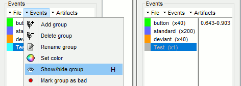
Channel events
Some events can be attached to only one or a few channels. This is useful for instance for reviewing clinical EEG recordings, where neurologists are tagging epileptic activity only on a subset of the channels.
- First select the channels of interest by clicking on them (the signals should turn red).
- Place the time cursor where you want to create the event (click on the white or grey areas of the figure, or use the shortcut Shift+Click).
Right-click anywhere on the figure > Add/delete channel event, or shortcut Ctrl+E.
The event marker appears directly on the selected channel, and the name of the channel appears in the list of event times (in the Brainstorm window).

Then you can deselect the channel (click again on it) or press the Escape key before creating a new event attached to a different channel.
- If no channel is selected, you can proceed in this alternate way: position the time cursor where you want to create the event, right-click directly on the channel to which to want to attach the event, and select "Add/delete channel event".
Notes
Additional comments can be added to the event, in case additional details should be displayed in the file viewer. This is mostly useful for reviewing clinical recordings as well.
Right-click on any event marker or event text (or double-click on it) > Edit notes.
Enter the text to display next to the marker.

Alternatively, you can double-click on the event in the list of event times (in the Brainstorm window).
HED tags
Hierarchical Event Descriptors (HED) provide a standardized and machine-readable way to describe events in neuroimaging datasets. Brainstorm now includes support for viewing, editing, validating, and using HED tags during analysis. More information can be found in the dedicated tutorial: HED tags.
Display modes
Three display modes are available for the event markers: dots, lines or hidden. Select the corresponding menu in the display options, or press CTRL+L multiple times.


Custom shortcuts
When reviewing long recordings and adding manually lots of events (eg. when marking manually epileptic spikes), using the menus presented above is not convenient because they require many mouse clicks.
Using the menu Events > Edit keyboard shortcuts, you can associate custom events to the key 1 to 9 of the keyboard. Define the name of the event type to create for each key, and then simply press the corresponding key to add/delete a marker at the current time position. Three options are available for each event type:
Simple: Create a simple event where the red time cursor is placed.
Full page: Create an extended event including the entire page of recordings, then move to the next page of recordings. This option was added for a specific application (sleep staging) that consists in labelling blocks of 30s through the entire file.
Extended: Create an extended event with the time window indicated on the right of the panel around the time cursor.
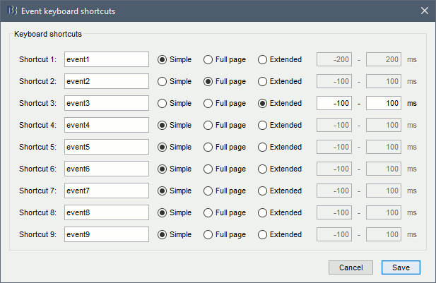
Saving modifications
Now you can delete all the event groups that you've just created and leave only the initial ones (button, standard, deviant): select the event groups and press Delete, or use the menu Events > Delete group.
When you close the continuous file viewer, or the last figure that shows a part of the raw file, the dataset is unloaded, the file is released and the memory is freed.
If you edited the events for this file, you are asked whether to save the modifications or not. If you answer "Yes", the modifications are saved only in the database link (Link to raw file), not in the original file itself. Therefore, you would see the changes the next time you double-click on the "link to raw file" again, but not if you open the original .ds file in another protocol or with an external program.
Note that events you edit are not automatically saved until that moment. As you would do with any other type of computer work, save your work regularly, to limit the damages of a program or computer crash. In the Record tab, use the menu File > Save modifications.
Other menus
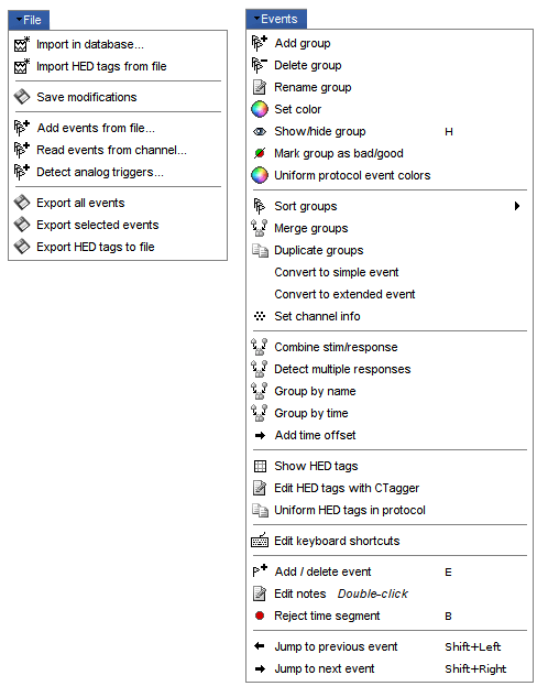
File
Import in database: Import blocks of the current continuous file into the database. Equivalent to a right click on the "Link to raw file" in the database explorer > Import in database.
Import HED tags from file: Import HED tags from a JSON sidecar file. See HED tags tutorial.
Save modifications: Save the modifications made to the events in the database link.
Add events from file: Import events from an external file. Many file formats are supported.
Read events from channel: Read the information saved during the acquisition in a digital auxiliary channel (eg. a stimulus channel) and generate events.
Detect analog triggers: Detect transition events in an external analog channel, such as the voltage of a photodiode exposed to light or a microphone recording a sound.
Export all events: Save all the events in an external file.
Export selected events: Same as "Export all events" but exports only the selected events.
Export HED tags to file: Save all the HED tags as a JSON sidecar file. See HED tags tutorial.
Events
Add group: Create a new group of events.
Delete group: Deletes the selected groups of events. Shortcut: Delete.
Rename group: Rename the selected group of events. Shortcut: double-click.
Delete group: Deletes the selected groups of events. Shortcut: Delete.
Set color: Change the color associated with an event group.
Show/hide group: Shows or hides selected groups of events. . Shortcut: H.
Mark group as bad: Add a tag "bad" in the event name, so that it is considered as bad segment.
Uniform protocol event color: Uses the current file as seed, and change the colors of indicated events in all the files in the Protocol.
Sort groups: Reorders the event groups by name, or by time of the first occurrence.
Merge groups: Merge two event groups into a new group. Initial groups are deleted. To keep them, duplicate them before merging.
Duplicate groups: Make a copy of the selected event groups.
Convert to simple events: Convert a group of extended events (several time points for each event), to simple events (one time point). An option window asks you whether to keep the first, middle, last sample or every sample of the extended events.
Convert to extended events: Convert simple events to segments of a fixed length.
Set channel info: Updates the channel information for the selected event groups.
Combine stim/response: Create new groups of events based on stim/response logic.
Example: Stimulus A can be followed by response B or C. Use this process to split the group A in two groups: AB, followed by B; and AC, followed by C.Detect multiple responses: Finds the multiple responses (events that are too close to each other)
Group by name: Combine different event groups by name.
Group by time: Combine simultaneous events and creates new event groups.
Add time offset: Adds a constant time to all the events in a group, to compensate for a delay.
Show HED tags: Print out the HED tags for the selected event groups.
Edit HED tags with CTagger: Open the CTagger GUI to create, edit or delete HED tags for the selected event groups. See HED tags tutorial.
Uniform HED tags in protocol: Aggregates all the unique HED tags for the selected event groups across all the files in the Protocol, then updates all the files in the protocols to these aggregated HED tags.
Edit keyboard shortcuts: Custom associations between keys 1..9 and events
Reject time segment: Mark the current time selection as bad.
Jump to previous/next event: Convenient way of browsing through all the markers in a group.
Shortcut: Shift + left/right
On the hard drive
The nodes "Link to raw file" you see in the database explorer are represented by .mat files on the hard drive. They contain all the header information extracted from the raw files, but do not contain a full copy of the recordings.
All the additional information created from the Brainstorm interface (event markers, bad channels, SSP projectors) are not saved back to the original raw files, they are only saved in the "Link to raw file". The names of these files start with the tag data_0raw_, they share the same structure as all the imported epochs (introduced later in the tutorials).
To explore the contents of these link files, right-click on them use the popup menus File > View file contents or File > Export to Matlab.
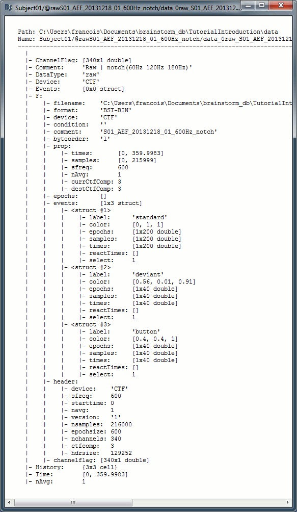
Link to raw file structure: data_0raw_*.mat
F: sFile structure, documents completely the continuous raw file, described below.
(for imported epochs, .F contains directly the MEG/EEG recordings [Nchannels x Ntime])Comment: String used to represent the file in the database explorer.
Time: First and last time points recorded in the continuous file.
ChannelFlag: [Nchannels x 1] list of good/bad channels (good=1, bad=-1)
DataType: Type of data stored in this file.
- 'raw' = Link to a continuous raw file
- 'recordings' = Imported epoch
Device: Acquisition system that recorded the dataset.
Events: Not used in the case of links.
T0: Not used in the case of links.
Leff: Effective number of averages = Number of input files averaged to produce this file.
History: Describes all the operations that were performed with Brainstorm on this file. To get a better view of this piece of information, use the menu File > View file history.
sFile structure: This structure is passed directly to all the input/output functions on continuous files.
filename: Full path to the continuous raw file.
format: Format of the continuous raw file.
device: Acquisition system that recorded the dataset. Same as Link.Device.
condition: Name of the folder in which this file is supposed to be displayed.
comment: Original file comment.
byteorder: Endianness, 'l' = Little Endian, 'b' = Big Endian
prop: Structure, basic properties of the recordings
times: First and last time points recorded in the continuous file.
sfreq: Sampling frequency
Leff: Number of files that were averaged to produce this file.
currCtfComp: Level of CTF compensation currently applied.
destCtfComp: Level of CTF compensation in which we want to view the file (usually: 3)
epochs: Array of structures used only in the case of continuous recordings saved as "epochs"
events: Array of structures describing the event markers in the file, one structure per event group:
label: Name of the event group
color: [r,g,b] Color used to represent the event group, in Matlab format
epochs: [1 x Nevt] Indicate in which epoch the event is located (index in the sFile.epochs array), or 1 everywhere for files that are not saved in "epoched" mode.
Nevt = number or occurrences of the event = number of markers in this grouptimes: [1 x Nevt] Time in seconds of each marker in this group (times = samples / sfreq), aligned on exact sample instants (times = round(times*sfreq)/sfreq).
For extended events: [2 x Nevt], first row = start, second row = endreactTimes: Not used anymore
select: Indicates if the event group should be displayed in the viewer.
channels: {1 x Nevt} Cell array of cell-arrays of strings. Each event occurrence can be associated with one or more channels, by setting .channels{iEvt} to a cell-array of channel names.
notes: {1 x Nevt} Cell-array of strings: additional comments for each event occurrence
hedTags: {1 x NhedTags} Cell-array of strings: HED tags for this event group.
t0: Timestamp with milliseconds to indicate the time 0s in the recording.
header: Structure describing additional header information, depending on the original file format.
channelflag: List of good/bad channels, same information as Link.ChannelFlag.
Useful functions
in_bst_data(DataFile, FieldsList): Read the structure for a data file.
Tutorial 8: Stimulation delays
Authors: Francois Tadel, Elizabeth Bock
The event markers that are saved in the data files might have delays. In most cases, the stimulation triggers saved by the acquisition system indicate when the stimulation computer requested a stimulus to be presented. After this request, the equipment used to deliver the stimulus to the subject (projector, screen, sound card, electric or tactile device) always introduce some delays. Therefore, the stimulus triggers are saved before the instant when the subject actually receives the stimulus.
For accurate timing of the brain responses, it is very important to estimate these delays precisely and if possible to account for them in the analysis. This tutorial explains how to correct for the different types of delays in the case of an auditory study, if the output of the sound card is saved together with the MEG/EEG recordings. A similar approach can be used in visual experiments using a photodiode.
Contents
Note for beginners
This entire tutorial can be considered as advanced. It is very important to correct for the stimulation delays in your experiments, but if you are not using any stimulation device, you do not need this information. However, if you skip the entire tutorial, you will have uncorrected delays and it will be more difficult to follow along the rest of the tutorials. Just go quickly through the actions that are required and skip all the explanations.
Documented delays
Reminder: The full description of this auditory dataset is available on this page: Introduction dataset.
Delay #1: Production of the sound
- The stimulation software generates the request to play a sound, the corresponding trigger is recorded in the stim channel by the MEG acquisition software.
- Then this request goes through different software layers (operating system, sound card drivers) and the sound card electronics. The sound card produces an analog sound signal that is sent at the same time to the subject and to MEG acquisition system. The acquisition software saves a copy of it in an audio channel together with the MEG recordings and the stim channel.
The delay can be measured from the recorded files by comparing the triggers in the stim channel and the actual sound in the audio channel. We measured delays between 11.5ms and 12.8ms (std = 0.3ms). These delays are not constant, we should adjust for them. Jitters in the stimulus triggers cause the different trials to be aligned incorrectly in time, hence "blurred" averaged responses.
Delay #2: Transmission of the sound
- The sound card plays the sound, the audio signal is sent with a cable to two transducers located in the MEG room, close to the subject. This causes no observable delay.
- The transducers convert the analog audio signal into a sound (air vibration). Then this sound is delivered to the subject's ears through air tubes. These two operations cause a small delay.
This delay cannot be estimated from the recorded signals: before the acquisition, we placed a sound meter at the extremity of the tubes to record when the sound is delivered. We measured delays between 4.8ms and 5.0ms (std = 0.08ms). At a sampling rate of 2400Hz, this delay can be considered constant, we will not compensate for it.
Delay #3: Recording of the signals
The CTF MEG systems have a constant delay of 4 samples between the analog channels (MEG/EEG, auditory,etc) and the digital channels (stim, buttons, etc), because of an anti-aliasing filter that is applied to the first and not the second. This translates here to a constant 'negative' delay of 1.7ms, meaning the analog channels are delayed when compared to the stim channels.
- Many acquisition devices (EEG and MEG) have similar hidden features, read correctly the documentation of your hardware before analyzing your recordings.

Evaluation of the delay
Let's display simultaneously the stimulus channel and the audio signal.
Right-click AEF#01 link > Stim > Display time series: The stim channel is UPPT001.
Right-click AEF#01 link > ADC V > Display time series: The audio channel is UADC001.
In the Record tab, set the duration of display window to 0.200s.
- Jump to the third event in the "standard" category.
We can observe that there is a delay of about 13ms between the time where the stimulus trigger is generated by the stimulation computer and the moment where the sound is actually played by the sound card of the stimulation computer (delay #1).
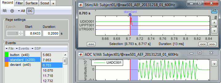
- What we want to do is to discard the existing triggers and replace them with new, more accurate ones created based on the audio signal. We need to detect the beginning of the sound on analog channel UADC001.
- Note that the representation of the oscillation of the sound tone is really bad here. The frequency of this standard tone is 440Hz. It was correctly captured by the original recordings at 2400Hz, but not in the downsampled version we use in the introduction tutorials. It should still be good enough for performing the detection of the stimulus.
Detection of the analog triggers
Detecting the standard triggers
Run the detection of the "standard" audio triggers on channel UADC001 for file AEF#01.
- Keep the same windows open as previously.
In the Record tab, select the menu File > Detect analog triggers.
This opens the Pipeline editor window with the process Events > Detect analog triggers selected. This window will be introduced later, for now we will just use it to configure the process options. Configure it as illustrated below:
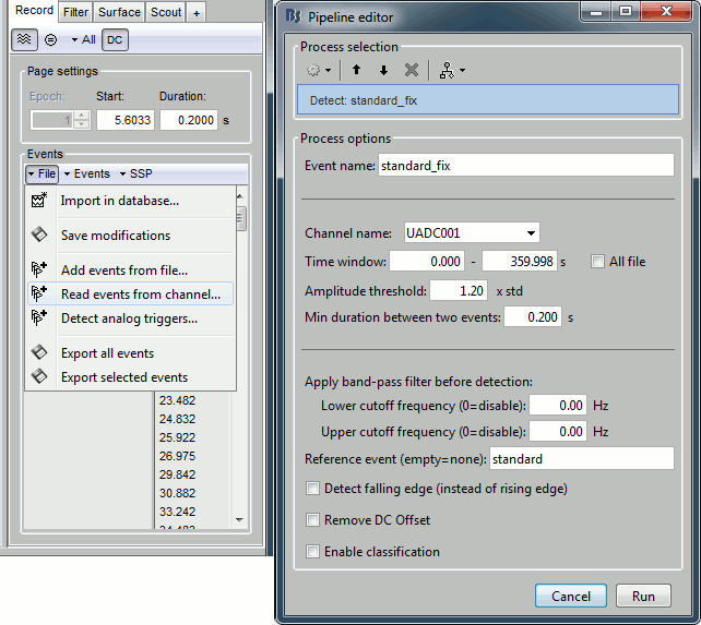
Explanation of the options (for future reference, you can skip this now):
Event name: Name of the new event category created to store the detected triggers.
We can start with the event "standard", and call the corrected triggers "standard_fix".Channel name: Channel on which to perform the detection (audio channel UADC001).
Time window: Time segment on which you want to detect analog triggers.
Leave the default time window or check the box "All file", it will do the same thing.Amplitude threshold: A trigger is set whenever the amplitude of the signal increases above X times the standard deviation of the signal over the entire file. Increase this value if you want the detection to be less sensitive.
Min duration between two events: If the event we want to detect is an oscillation, we don't want to detect a trigger at each cycle of this oscillation. After we detect one, we stop the detection for a short time. Use a value that is always between the duration of the stimulus (here 100ms) and the inter-stimulus interval (here > 700ms).
Apply band-pass filter before the detection: Use this option if the effect you are trying to detect is more visible in a specific frequency band. In our case, the effect is obvious in the broadband signal, we don't need to apply any filter.
Reference: If you have an approximation of the triggers timing, you can specify it here. Here we have the events "standard" and we want to detect a trigger in their neighborhood.
If we do not use this option, the process creates only one new group with all the audio signals, without distinction between the deviant and standard tones.Detect falling edge (instead of rising edge): Detects the end of the tone instead of the beginning.
Remove DC offset: If the signal on which we perform the detection does not oscillate around zero or has a high continuous component, removing the average of the signal can improve the detection. This should be selected when using a photodiode with a pull-up resistor.
Enable classification: Tries to automatically classify the different types of events that are detected based on the morphology of the signal in the neighborhood of the trigger.
Results of the detection
- Navigate through a few of the new "standard_fix" events to evaluate if the result is correct. You can observe that the corrected triggers are consistently detected after the rising portion of the audio signal, two samples after the last sample where the signal was flat.
This means that we are over-compensating delay #1 by 3.3ms. But at least this delay is constant and will not affect the analysis. We can count this as a constant delay of -3.3ms.
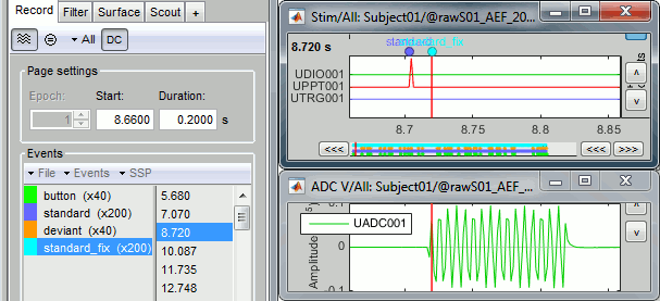
Detecting the deviant triggers
- Repeat the same operation for the deviant tones.
In the Record tab, select the menu File > Detect analog triggers.
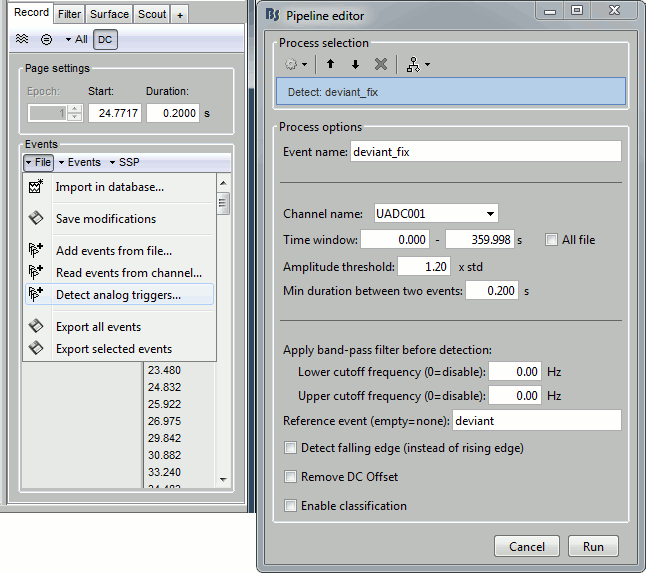
Some cleaning
- We will use the corrected triggers only, we can delete the original ones to avoiding any confusion.
Delete the event groups "deviant" and "standard" (select them and press the Delete key).
- Rename the group "deviant_fix" into "deviant" (double-click on the group name).
- Rename the group "standard_fix" into "standard".
Close all: Answer YES to save the modifications.
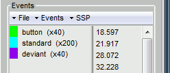
Repeat on acquisition run #02
Repeat all the exact same operations on the link to file AEF#02:
Right-click AEF#02 link > Stim > Display time series: The stim channel is UPPT001.
Right-click AEF#02 link > ADC V > Display time series: The audio channel is UADC001.
In the Record tab, select menu File > Detect analog triggers: standard_fix
In the Record tab, select menu File > Detect analog triggers: deviant_fix
- Check that the events are correctly detected.
Delete the event groups "deviant" and "standard" (select them and press the Delete key).
- Rename the group "deviant_fix" into "deviant" (double-click on the group name).
- Rename the group "standard_fix" into "standard".
- Close all: Answer YES to save the modifications.
Delays after this correction
We compensated for the jittered delays (delay #1), but not for hardware delays (delay #2). Note that delay #3 is no longer an issue since we are not using the orginal stim markers, but the more accurate audio signal. The final delay between the "standard_fix" triggers and the moment when the subject gets the stimulus is now delay #2 and the over-compensation.
Final constant delay: 4.9 - 3.3 = 1.6ms
We decide not to compensate for this delay because it is very short and does not introduce any jitter in the responses. It is not going to change anything in the interpretation of the data.
Detection of the button responses
The subject presses a button with the right index finger when a deviant is presented. We don't really need to correct this category of events because it is already correct. You can skip this section if you are not interested in parsing digital channels.
The digital channel Stim/UDIO001 contains the inputs from the response button box (optic device, negligible delay). Each bit of the integer value on this channel corresponds to the activation of one button. We can read this channel directy to get accurate timing for the button presses.
Right-click AEF#01 link > Stim > Display time series: The response channel is UDIO001.
In the Record tab: Set the page duration to 3 seconds.
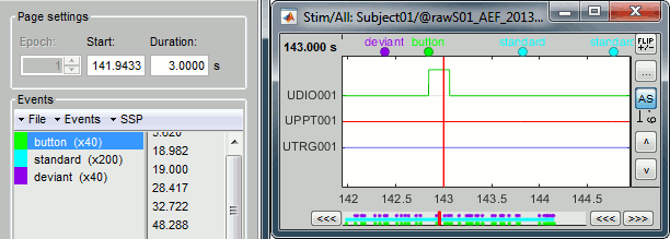
Note on the DC removal: You may see the base value of the UDIO001 channel "below" the zero line. This is an effect of the DC correction that is applied on the fly to the recordings. The average of the signals over the current page is subtracted from them. To restore the real value you can uncheck the [DC] button in the Record tab. Atlernatively, just remember that the reference line for a channel doesn't necessarily mean "zero" when the DC removal option is on.
In the Record tab, select menu File > Read events from channel: UDIO001 / Value
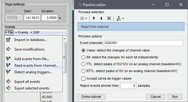
Reject events shorter than X samples: This option is not needed here, but can become useful when the transitions between the values of the stim channels are not as clean as the sharp steps in this tutorial dataset. For example:
- The individual bits are not changing exactly at the same time,
- Values added (bit-wise) at transitions between 2 non-zero values when downsampling (e.g. CTF),
- "Button bouncing": non-ideal behavior of any switch which generates multiple transitions from a single input.
You get a new event category 64, this is the value of the UDIO001 at the detected transitions. There are 40 of them, one for the each button press. We can use this as a replacement for the original button category.
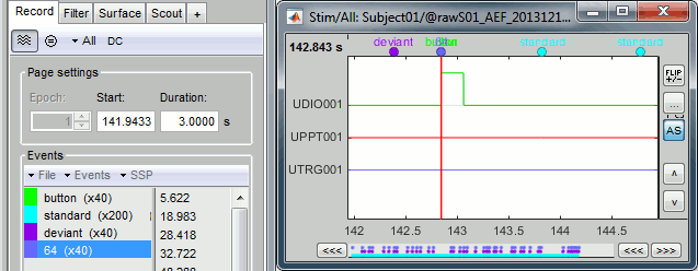
To make things clearer: delete the button group and rename 64 into button.

- Close all: Answer YES to save the modifications.
- Optionally, you can repeat the same operation for the other run, AEF#02. But we will not use the "button" markers in the analysis, so it is not very useful.
- Note that these events will have delay #3 (when compared to MEG/EEG) since they are recorded on a digital channel.
Another example: visual experiments
We have discussed here how we could compensate for the delays introduced in an auditory experiment using a copy of the audio signal saved in the recordings. A similar approach can be used for other types of experiments. Another typical example is the use a photodiode in visual experiments.
When sending images to the subject using a screen or a projector, we usually have jittered delays coming from the stimulation computer (software and hardware) and due to the refresh rate of the device. These delays are difficult to account for in the analysis.
To detect accurately when the stimulus is presented to the subject, we can place a photodiode in the MEG room. The diode produce a change in voltage when presented with a change in light input, for example black to white on the screen. This is typically managed with a small square of light in the corner of the stimulus screen - turning white when the stimulus appears on the screen and then black at all other times. The signal coming from this photodiode can be recorded together with the MEG/EEG signals, just like we did here for the audio signal. Depending on the photodiode, it is recommended to use a pull-up resistor when recording the signal. Then we can detect the triggers on the photodiode output channel using the menu "detect analog triggers", including the use of the 'Remove DC offset' option.
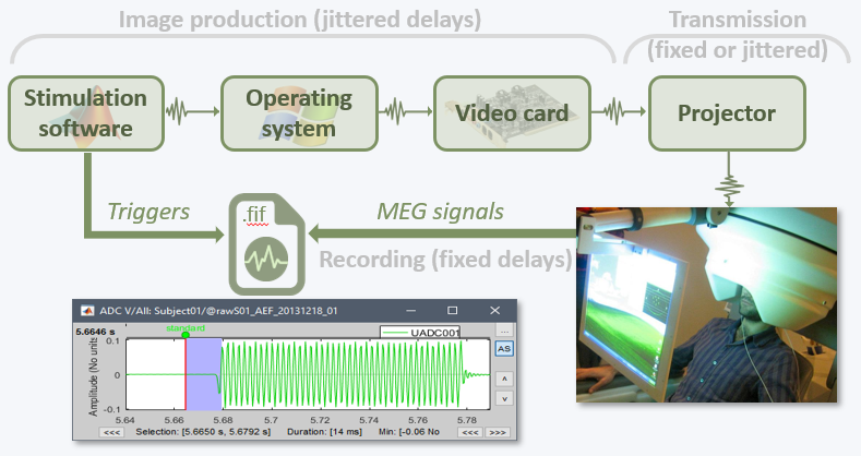
Tutorial 9: Select files and run processes
Authors: Francois Tadel, Elizabeth Bock, Sylvain Baillet
The Brainstorm window includes a graphical batching interface. With the two tabs Process1 and Process2 in the lower part of the window, you can select files from the database explorer and assemble a processing pipeline. Most of the operations available in the interface can also be executed this way, including everything we've been doing with Brainstorm so far.
On the other hand, some features are only available this way. It is the case for the frequency filters we will need for the pre-processing of our auditory recordings. This tutorial is a parenthesis to explain how to select files and run processes, we will resume with the cleaning of the recordings in the next tutorial.
Contents
Selecting files to process
The tab Process1 contains a empty box in which you can drag and drop any number of files or folders from the database explorer. The easiest way to understand how it works is to try it.
- Try to drag and drop, in Process1, all the nodes you currently have in your database explorer.
- You will see that it accepts all the folders and all the recordings, but not the channel files.
- When you add a new node, the interface evaluates the number of files of the selected type that each of them contain. The number in the brackets next to each node represents the number of data files that were found in them.
On top of the list, a comment shows the total number of files that are currently selected.
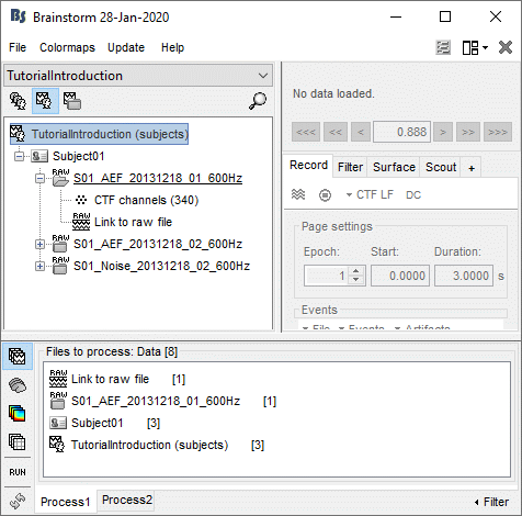
- The buttons on the left side allow you to select what type of file you want to process: Recordings, sources, time-frequency, other. When you select another button, all the counts are updated to reflect the number of files of the selected type that are found for each node.
Right now, if you select another file type, it would show only "0" everywhere because there are no sources or time-frequency decompositions available in the database yet.
- To remove files from the Process1 list:
Select the nodes to remove (holding Shift or Ctrl key) and press the Delete key.
Right-click on the list > Clear list
Filter by name
When you have lots of files in a folder, like multiple source reconstructions or time-frequency files for each trial, it is difficult to grab just the ones you are interested in. After selecting your folders in the Process1 box, you can refine the selection with the Filter search box at the bottom-right corner of the window.
The example below shows how to select the data files corresponding to the noise recordings: by typing "Noise" in the search box and selecting the option "Search file paths". We cannot perform the search "by name" because all the data files have the same name "Link to raw file".
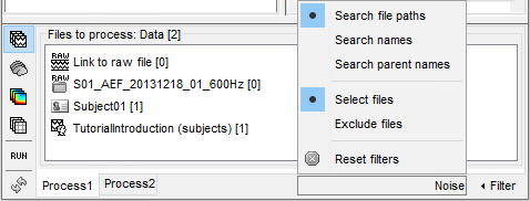
Reminder: To see the file name corresponding to a node in the database, leave your mouse over it for a few seconds. You can do this both in the database explorer and the Process1 list.

The options offered in the Filter menu are:
Search file paths: Look for the string in the full file paths (including their relative path).
Search names: Look for the string in the names of the files, ie. what is displayed in the database explorer to represent them (the .Comment field).
Search parent names: Extends the search to the name of the parent files (applicable only to source and time-frequency files, which can depend on a data file).
Select files: Only the files that contain the string are selected.
Exclude files: Only the files that DO NOT contain the string are selected.
Reset filters: Removes the current file filters applied on Process1 and Process2.
Case insensitive: Note that the search is not sensitive to case.
Boolean logic: You can combine different keywords to make a more precise search using advanced search queries. See the following section for more information.
Selecting processes
- Clear the file list and the search filters.
Select all three datasets we have linked to our protocol.
You can select the three "link to raw file" nodes, the three folders or the entire subject node.Click on the [Run] button at the bottom-left corner of the Process1 tab.
The Pipeline editor window appears. You can use it to create an analysis pipeline, i.e., a list of processes that are applied to the selected files one after the other. The first button in the toolbar shows the list of processes that are currently available. If you click on a menu, it's added to the list.
- Some menus appear in grey. This means that they are not designed to be applied to the type of data that you have in input, or at the end of the current pipeline.
In the current example, we have a file with the type "continuous raw recordings", so we have access mostly to menus to manipulate event markers, run cleaning procedures and import data blocks. You can recognize a few operations that we executed in the previous tutorials: "Event > Read from channel" and "Event > Detect analog triggers".
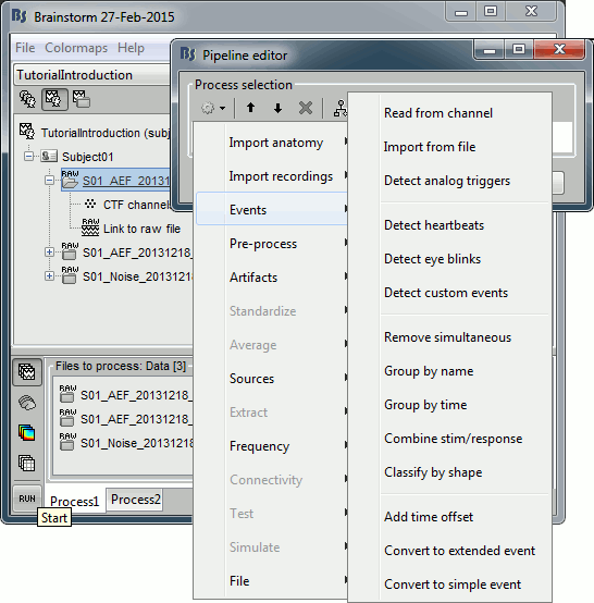
- When you select a process, a list of options specific to this process is shown in the window.
To delete a process: Select it and press the Delete key, or use the [X] button in the toolbar.
- After selecting a first process, you can add another one. The output of the first process will be passed to the second process without giving back the control to the user. This is how you can build a full analysis pipeline with the interface.
- After adding a few processes, you can move a process up or down in the pipeline with the [up arrow] and [down arrow] buttons in the toolbar. Click on a process in the pipeline to edit its options.
- Select and delete a few processes to understand how this interface works. Just do not click on RUN.
Plugin structure
All the menus available in the pipeline editor are actually plugins for Brainstorm. The processes are functions that are independent from each other and automatically detected when starting Brainstorm.
Any Matlab script that is added to the plugin folder (brainstorm3/toolbox/process/functions/) and has the right format will automatically be detected and made available in the GUI. This mechanism makes it easy for external contributors to develop their own code and integrate it in the interface.
More information: How to write your own process
To see where the function corresponding to a process is on the hard drive: select the process in the pipeline editor, then leave your mouse for a few seconds over its title.
Note for beginners
Everything below is advanced documentation, you can skip it for now.
Search Database
Sometimes when working with huge protocols, you can get lost in the size of your database tree. While filtering from the process box as introduced in the previous section is one way to select the files you are looking for, we have introduced a more straightforward approach to search for file(s) in your database. At the right below the protocol selection dropdown, you can click on the magnifying glass to open up the search dialog.
From there, you can create a new search query from the GUI, or type / paste an existing search query string (see the following section for more details). Let's select "New Search" to create a new query from the GUI.
From this menu, you can create a search query to apply on your active protocol. It has different options:
Search by: The file metadata to use for the search.
- Name: Name of the file in Brainstorm
- File type: Type of the file, see dropdown when selected for possible values
- File path: Path of the file in the Brainstorm database folder
- Parent name: Name of any parent file in the database tree (e.g. Subject or Folder)
Equality: Type of equality to apply.
- Contains: File metadata contains the entered value
- Contains (case): Same as contains, but case sensitive
- Equals: Exact equality, the file metadata is equal to the entered value
- Equals (case): Same as equals, but case sensitive
Not: Whether to invert the selected equality, e.g. DOES NOT CONTAIN vs CONTAINS.
Search for: The value to search for.
Remove: To remove the search row if not needed anymore.
+ and: To add a search row, with the AND boolean logic. If you have two rows A and B, then the returned files will match both search A and B.
+ or: To add a search row, with the OR boolean logic. If you have two rows A and B, then the returned files will match both search A or B.
In the above example, we are looking for raw files (File type = Raw data) whose parent name contains the word "noise". This allows us to search for raw noise recordings.
Notice that you now have multiple tabs in your Brainstorm database. The "Database" tab contains all files in your protocol, whereas the "noise" tab only contains the files that pass the search and their parents. You can have multiple searches/tabs active so that you can easily create pipelines by dragging and dropping different search results in the process box. Do keep in mind that if you drag and drop a parent object in the process box (e.g. Subject01) with an active search, only files that pass the active search will be processed by the pipeline.
Once a search is created, you can interact with it in different ways. You can right click on the tab and Edit the search on the fly from the GUI, Copy the search to clipboard as a query string to use it in a script, or Close the search.
You can also click on the magnifying glass when a search is active to get more options such as Saving the search for later use and Generating a process call to apply this search in a script.
If you click Generate process call, a line of script will be generated for you to use your search query as a process in a script. It will also be copied to clipboard.
Notice that your search was created to a query string:
([parent CONTAINS "noise"] AND [type EQUALS "RawData"])
This advanced query syntax is described in the following section.
Advanced search queries
For advanced users, you can write more complex search queries that can combine multiple keywords and types of keywords using boolean logic. You can do this using the Brainstorm search GUI and then copy your search as text to re-use later. These queries work for both database searches and process filters. The syntax is rigid such that the order of the commands is important, so we recommend you use the search GUI whenever possible to avoid errors. Search queries can contain the following types of elements:
Search parameters: These are simple searches that are on a specific type of value. They need to be written in [square brackets]. They look like the following:
- [searchFor EQUALITY NOT "value"]
SearchFor: Which field of the files metadata to search for It can have the following values, in lower case:
- Name: Searches using the file name in Brainstorm
- Type: Searches using the file type in Brainstorm
- Path: Searches using the file path in the Brainstorm database folder
- Parent: Searches using the parents name in the Brainstorm database tree
Equality: The type of equality you want to use to compare the file value to the searched value. It can have the following values, in upper case:
- CONTAINS: Whether the searchFor field contains the text "value"
- CONTAINS_CASE: Same as CONTAINS, but case sensitive
- EQUALS: Whether the searchFor field exactly equals the text "value"
- EQUALS_CASE: Same as EQUALS, but case sensitive
NOT: (optional) add this reserved keyword to return the opposite results of the search, so for example, all files that do NOT CONTAIN the text "value".
"value": the text you want to search for, in double quotes.
Boolean operators: These are used to group together search parameters and search blocks using boolean logic. Considering search parameters a, b and c, the following will return files that pass searches a and a, or does not pass search c:
- (a AND b) OR NOT c
AND: This combines search parameters and blocks such that both conditions have to be met.
OR: This combines search parameters and blocks such that either conditions have to be met
NOT: This precedes a search block or parameter such that the condition result is reversed. So if a condition had to be met, it now has to not be met.
Important note: AND and OR operators cannot be mixed together (you cannot have both in the same search block), because otherwise it creates uncertainties.
Search blocks: These are combinations of search parameters and boolean operators, wrapped in (round brackets). You cannot have different boolean operators in the same block
Example
(([name CONTAINS "test1"] AND [type EQUALS "Matrix"]) OR NOT [parent CONTAINS "test2"])
Effect: This will match all matrix files containing text "test1" or all files whose parent docontains the text "test2".
Limitations of the GUI
The GUI does not support multiple nested search blocks. It only allows for one OR block followed by one AND block. If your query is more advanced than this, you will not be able to edit it with the search GUI. We recommend you use the process filter box instead.
Saving a pipeline
After preparing your analysis pipeline by listing all the operations to run on your input files, you can either click on the [Run] button, or save/export your pipeline. The last button in the the toolbar offers a list of menus to save, load and export the pipelines.
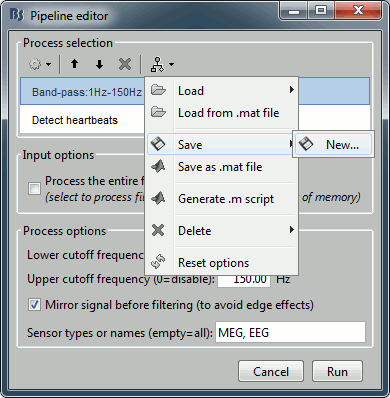
Load: List of pipelines that are saved in the user preferences on this computer.
Load from .mat file: Import a pipeline from a pipeline_...mat file.
Save: Save the pipeline in the user preferences.
Save as .mat matrix: Exports the pipeline as Matlab structure in a .mat file. Allows different users to exchange their analysis pipelines, or a single user between different computers.
Generate .m script: This option generates a Matlab script.
Delete: Remove a pipeline that is saved in the user preferences.
Reset options: Brainstorm automatically saves the options of all the processes in the user preferences. This menu removes all the saved options and sets them back to the default values.
Automatic script generation
Here is the Matlab script that is generated for this pipeline.
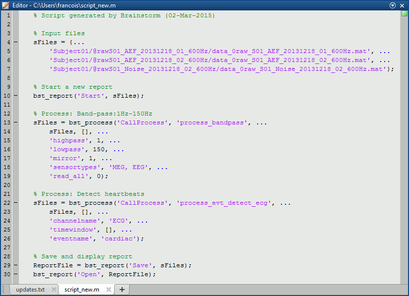
Reading this script is easy: input files at the top, one block per process, one line per option. You can also modify them to add personal code, loops or tests. Many features are still missing in the pipeline editor, but the generated scripts are easy enough for users with basic Matlab knowledge to edit and improve them.
Running this script from Matlab or clicking on the [Run] button of the pipeline editor produce exactly the same results. In both cases you will not have any interaction with the script, it could be executed without any direct supervision. You just get a report in the end that describes everything that happened during the execution.
These scripts cannot be reloaded in the pipeline editor window after being generated. If you work on a long analysis pipeline, save it in your user preferences before generating the corresponding Matlab script.
Process: Select files with tag
Since we are discussing the file selection and the pipeline execution, we can explore a few more available options. We have seen how to filter the files in the Process1 box using the Filter search box. We can get to the exact same result by using the process File > Select files: By tag before the process you want to execute, to keep only a subset of the files that were placed in the Process1 list.
It is less convenient in interactive mode because you don't immediately see the effect of your file filter, but it can be very useful when writing scripts. You can also combine search constraints by adding the same process multiple times in your pipeline, which is not possible with the search box.
- Make sure you still have the three datasets selected in the Process1 list.
Select the process: File > Select files: By tag
- Select the options: Search: "Noise", Search the file names, Select only the files with the tag.
Click on [Run] to execute the process.
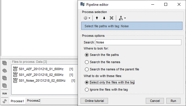
- This process is useless if not followed immediately by another process that does something with the selected files. It does nothing but selecting the file, but we can observe that the operation was actually executed with the report viewer.
Report viewer
Everytime the pipeline editor is used to run a list of processes, a report is created and logs all the messages that are generated during the execution. These reports are saved in the user home folder: $HOME/.brainstorm/reports/.
The report viewer shows, as an HTML page, some of the information saved in this report structure: the date and duration of execution, the list of processes, and the input and output files. It reports all the warnings and errors that occurred during the execution.
The report is displayed at the end of the execution only if there were more than one process executed, or if an error or a warning was reported. In this case, nothing is displayed.
You can always explicitly open the report viewer to show the last reports: File > Report viewer.
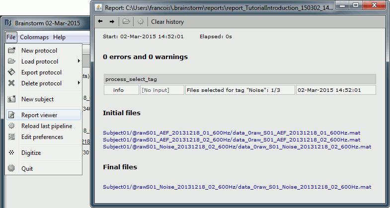
When running processes manually from a script, the calls to bst_report explicitly indicate when the logging of the events should start and stop.
You can add images to the reports for quality control using the process File > Save snapshot, and send the final reports by email with the process File > Send report by email.
With the buttons in the toolbar, you can go back to the previous reports saved from the same protocol.
More information: Scripting tutorial
Error management
Select the same files and same process: File > Select files: By tag
- Note that the options you used during the previous call are now selected by default.
Instead of "Noise", now search for a string that doesn't exist in the file name, such as "XXXX".
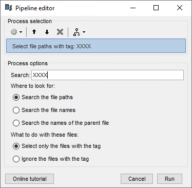
Click on [Run] to execute the process. You will get the following error.
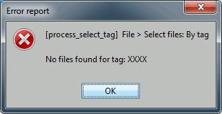
If you open the report viewer, it should look like this.
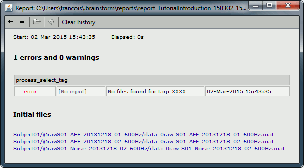
Control the output file names
If you are running two processes with different parameters but that produce exactly the same file paths and file names, you wouldn't be able to select them with this process. But immediately after calling any process, you can add the process File > Add tag to tag one specific set of files, so that you can easily re-select them later.
Example: You run the time-frequency decomposition twice with different options on the same files, tag the files after calculating them with different tags.
Additional documentation
Tutorial: Scripting
Tutorial: How to write your own process
Tutorial 10: Power spectrum and frequency filters
Authors: Hossein Shahabi, Francois Tadel, Elizabeth Bock, John C Mosher, Richard Leahy, Sylvain Baillet
We are now going to process our continuous recordings to remove the main sources of noise. Typically, we can expect contaminations coming from the environment (power lines, stimulation equipment, building vibrations) and from the subject (movements, blinks, heartbeats, breathing, teeth clenching, muscle tension, metal in the mouth or the body). In this tutorial, we will focus first on the noise patterns that occur continuously, at specific frequencies.
We can correct for these artifacts using frequency filters. Usually we prefer to run these notch and band-pass filters before any other type of correction, on the continuous files. They can be applied to the recordings without much supervision, but they may create important artifacts at the beginning and the end of the signals. Processing the entire continuous recordings at once instead of the imported epochs avoids adding these edge effects to all the trials.
Contents
- Evaluation of the noise level
- Interpretation of the PSD
- Elekta-Neuromag and EEG users
- Apply a notch filter
- Evaluation of the filter
- Some cleaning
- Note for beginners
- What filters to apply?
- When to apply these filters?
- Filter specifications: Low-pass, high-pass, band-pass
- Filter specifications: Notch
- Filter specifications: Band-stop
- On the hard drive
- Additional documentation
Evaluation of the noise level
Before running any type of cleaning procedure on MEG/EEG recordings, we always recommend to start with a quick evaluation of the noise level. An easy way to do this is to estimate the power spectrum of all the signals over the entire recordings.
- Clear the list of files in the Process1 tab.
Select the three datasets we have linked to our protocol.
You can select the three "link to raw file" nodes, the three folders or the entire subject node.

- Click on [Run] to open the pipeline editor window.
Select the process "Frequency > Power spectrum density (Welch)"
This process evaluates the power of the MEG/EEG signals at different frequencies, using the Welch's method (see Wikipedia or MathWorks). It splits the signals in overlapping windows of a given length, calculates the Fourier Transform (FFT) of each of these short segments, and averages the power of the FFT coefficients for all the overlapping windows.
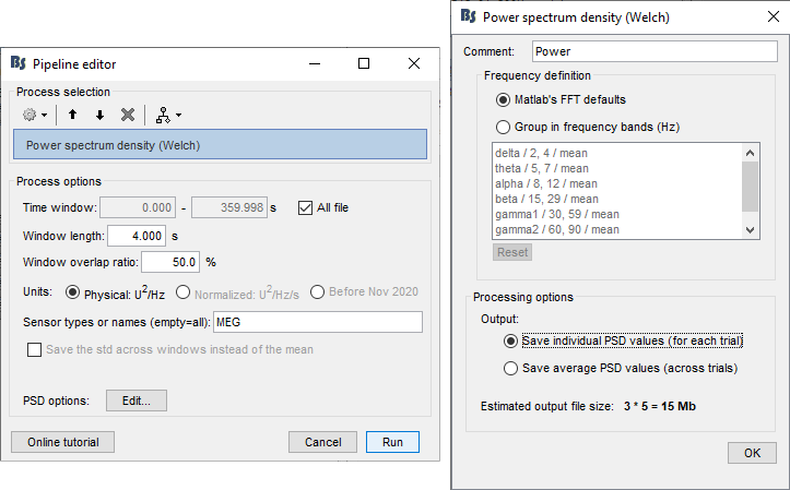
- Set the options as follows (click on [Edit] for the additional options):
Time window: [All file]
Portion of the input file you want to use for estimating the spectrum.
It is common to observe huge artifacts at the beginning or the end of the recordings, in this case you should exclude these segments from the calculation of the PSD.
In practice, using just the first 100s or 200s of the file can give you a good enough impression of the quality of the recordings.Window length: 4 seconds
Estimator length = length of the overlapping time windows for which we calculate the FFT. The number of time samples in the estimator is the same as the number of frequency bins in the output file. Increasing this parameter increases the output frequency resolution (distance between two frequency bins) but degrades the stability of the estimator, as it also decreases the total number of averaged time windows. A Hamming window is applied to each estimator window before the computation of the FFT. See forum post: Effect of window length on the PSDOverlap: 50%
How much overlap do we want between two consecutive time windows.Units: Physical: U^2/Hz
Scaling of the spectrum. This only affects the values on the Y axis of the spectrum. Physical units should be used in most cases.
"Normalized" gives normalized frequencies from 0 to 2pi (Hz·s).
"Before Nov 2020" reproduces the older Brainstorm spectrum scaling (see this forum post).Sensor types or names: MEG
Defines the list of channels (names or types) on which you want to apply the process.Frequency definition: Matlab's FFT default
You have the option to directly use the frequency binning returned by the FFT, or run an additional step of averaging these bins in larger frequency bands. Note that you can freely edit these frequency bands.Output: Save individual PSD value.
This option will separately estimate the PSD for each of the three files in input, and create three files in output. If you select the other option (save average), it calculates the same three files but averages them on the fly and saves only one file in the database.Implementation details: See function brainstorm3/toolbox/timefreq/bst_psd.m
- Click on [Run] to start the execution of the process.
Troubleshooting: If you get "Out of memory" errors, try to run this PSD estimation on a shorter time segment. For example, set the time window to [0,100s] instead of the full file. This process starts by loading all the needed recordings in memory, you might not have enough memory available on your system to fit the entire dataset.
It produces three new files, that appear as "depending" on the three datasets. The comments of the files indicate how many overlapping windows could be used to estimate the PSD. "179/4000ms" means 179 windows of 4s each (total 716s). With the 50% overlap, it sums up to a little less than 2x the file length (360s).
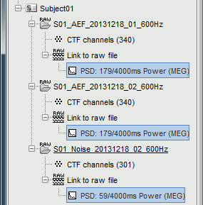
Interpretation of the PSD
File: AEF#01
Double-click on the new PSD file for run #01 to display it (or right-click > Power spectrum).
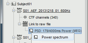
- The power spectrum is displayed in a figure similar to the time series, but the X axis represents the frequencies. Most of the shortcuts described for the recordings are also valid here. Clicking on the white parts of the figure or using the arrow keys of the keyboard move the frequency cursor. The current frequency can also be controlled with a new slider displayed in the Brainstorm window, just below the time panel.
Each black line represents the power spectrum for one channel. If you click on a channel, it gets highlighted in red. Click again for deselecting. Right-click on a selected channel to read its name.
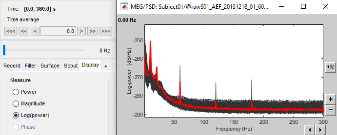
The frequency resolution of this power spectrum, ie. the distance between two frequency bins represented in this figure, is about 0.15Hz. This precision depends on the length of the estimator window you used. The FFT is computed on the number of time samples per window (4s*600Hz), rounded to the next power of 2 (nextpow2), and represents the full spectrum of the file (0-600Hz).
Frequency resolution = sampling_freq / 2^nextpow2(estimator_length*sampling_freq) = 0.1465 Hz- The shape of this graph is normal, it does not indicate anything unexpected:
Peaks related with the subject's alpha rhythms: around 10Hz and 20Hz.
Peaks related with the power lines: 60Hz, 120Hz and 180Hz.
These datasets were recorded in Canada, where the alternating powerline current is delivered at 60Hz. In Europe you would observe similar peaks at 50Hz, 100Hz and 150Hz.
- Add a topography view for the same file, with one of the two methods below:
Right-click on the PSD file > 2D Sensor cap.
Right-click on the spectrum figure > 2D Sensor cap (shortcut: Ctrl+T)
Scroll in frequencies to see the spatial distribution of each frequency bin:

- We have already identified two artifacts we will need to remove: the eye movements and the 60Hz+harmonics from the power lines.
File: AEF#02
Open the spectrum view for the run AEF#02.
To view the signal units instead of dB, select Display Tab > Measure > Power. Then from the display options icon on the right of the figure, select Amplitude > Log scale
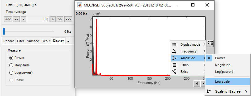
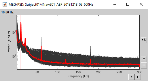
Add a 2D sensor cap view for the same file. Scroll to zoom in/out.
To display the sensor names, right-click on the figure > Channels > Display sensors.- This spectrum looks very similar to the run #01: same alpha and power line peaks.
Additionally, we observe higher signal power between 30Hz and 100Hz on many occipital sensors. This is probably related to some tension in the neck muscles due to an uncomfortable seating position in the MEG. We will see later whether these channels need to be tagged as bad or not.

File: Noise recordings
Open the spectrum view for the noise recordings.
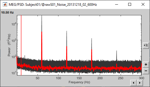
- This shows the power spectrum of the signals that are recorded when there is no subject in the MEG room. It gives a good and simple representation of the instrumental noise. If you had one bad MEG sensor, you would see it immediately in this graph. Here everything looks good.
X Log-scale
One option is worth mentioning when displaying power spectra: the logarithmic scale for the X axis. In the diaply options for the PSD figure > Frequency > Log scale. It is sometimes better adapted to represent this type of data than a linear scale (especially with higher sampling frequencies).
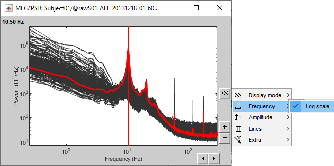
Elekta-Neuromag and EEG users
The Elekta-Neuromag MEG systems combine different types of sensors with very different amplitude ranges, therefore you would not observe the same types of figures. Same thing for EEG users, this might not look like what you observe on your recordings.
For now, keep on following these tutorials with the example dataset to learn how to use all the Brainstorm basic features. Once you're done, read additional tutorials in the section "Other analysis scenarios" to learn about the specificities related with your own acquisition system.
Apply a notch filter
This filter has been updated in 2019. In the new configuration, the user can define the 3-dB bandwidth of the filter. Please consider that a smaller bandwidth means a sharper filter which in some cases makes filter unstable. In case you want to reproduce the old filter, you can check the box "Use old filter implementation". The 3-dB bandwidth is not applicable to the old configuration.
For illustration purposes, we will now run a frequency filter to remove the 60Hz+harmonics from the continuous files. Notch filters are adapted for removing well identified contaminations from systems oscillating at very stable frequencies.
Keep all the three datasets selected in the Process1 box.
Remember to always apply the same filters on the subject recordings and the noise recordings.- Click on [Run] to open the Pipeline editor.
Run the process: Pre-process > Notch filter
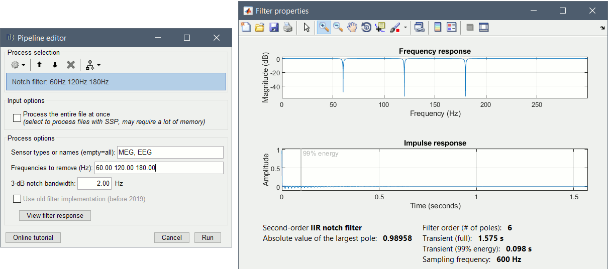
Process the entire file at once: NO
Sensor types or names: MEG
Frequencies to remove: 60, 120, 180 Hz
3-dB notch bandwidth: 2 Hz
- The higher harmonics (240Hz) are not clearly visible, and too high to bother us in this analysis.
This process creates three new datasets, with additional "notch" tags. These output files are saved directly in the Brainstorm database, in a binary format specific to Brainstorm (.bst).
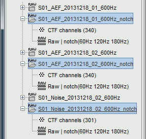
- If you delete the folders corresponding to the original files (before the filter), your original recordings in the .ds folders are not altered. If you delete the folders corresponding to the filtered files, you will lose your filtered recordings in .bst format.
To check where the file corresponding to a "Link to raw file" is actually saved on the hard drive, right-click on it > File > Show in file explorer.
Important: This is an optional processing step. Whether you need this on your own recordings depends on the analysis you are planning to run on the recordings (see advanced sections below).
Evaluation of the filter
Right-click on the Process1 list > Clear list.
Drag and drop the three filtered files in Process1.
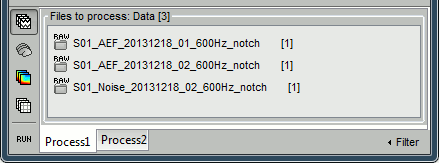
Run again the PSD process "Frequency > Power spectrum density (Welch)" on the new files, with the same parameters as before, to evaluate the quality of the correction.
Double-click on the new PSD files to open them.
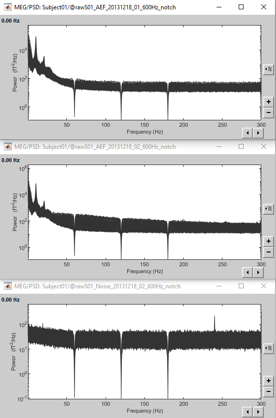
Scroll to zoom in and observe what is happening around 60Hz (before / after).
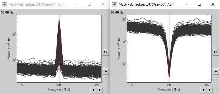
See below an example of how this filter can affect the time series: top=before, bottom=after.
We show the reference sensor BR2 because it shows a lot more 60Hz than any MEG sensor (sensor type "MEG REF"), ie. oscillations with a period of 16.7ms.
Note the edge effect at the beginning of the signal: the signals below are 1.5s long, the notch filter at 60Hz is visibly not performing well during the first 500ms (blue window).
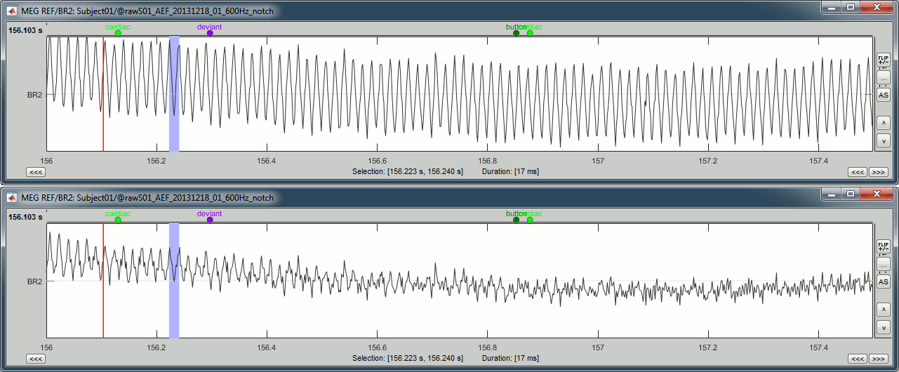
If you look in the list of events, you would see a new category "transient_notch". This corresponds to the time period during which can expect significant edge effects due to the filtering. Brainstorm doesn't mark these blocks as bad by default, you would have to do it manually - you will see how to do this in one of the following tutorials. In the case of this dataset, the transient duration is much shorter than the delay before the first stimulation, so not relevant in our processing pipeline. See the advanced sections below for more details about the estimation of this transient duration.
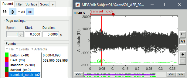
Some cleaning
To avoid any confusion later, delete the links to the original files:
Select the folders containing the original files and press Delete (or right-click > File > Delete).
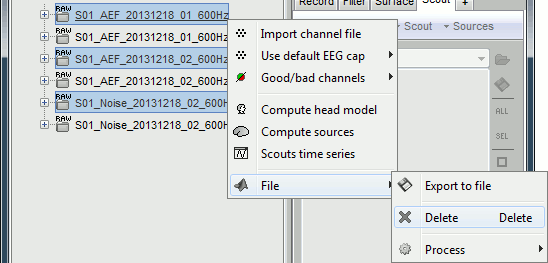
Always read the confirmation messages carefully, you will avoid some bad surprises.

This is what your database explorer should look like at the end of this tutorial:
Note for beginners
Everything below is advanced documentation, you can skip it for now.
What filters to apply?
The frequency filters you should apply depend on the noise present in your recordings, but also on the type of analysis you are planning to use them for. This sections provides some general recommendations.
High-pass filter
Purpose: Remove the low frequencies from the signals. Typically used for:
Removing the arbitrary DC offset and slow drifts of MEG sensors (< 0.2Hz),
Removing the artifacts occurring at low frequencies (< 1Hz, e.g. breathing or eye movements).
Warnings:
- Edge effects: Transient effects you should discard at the start and end of each filtered signal because the filtering window extends into time periods outside those for which you have data.
- Avoid using on epoched data: You need long segments of recordings to run a high-pass filter.
- Be careful with the frequency you choose if you are studying cognitive processes that may include sustained activity in some brain regions (eg. n-back memory task).
Low-pass filter
Purpose: Remove the high frequencies from the signals. Typically used for:
- If the components of interest are below for example 40Hz, you may discard the faster components in the signal by applying a low-pass filter with a frequency cutoff below 40Hz.
- Removing strong noise occurring at high frequencies (eg. muscle contractions, stimulators).
- Display averages: In an event-related design, you will import and average multiple trials. You may low-pass filter these averages for display and interpretation purposes.
- Statistics: In an event-related study with multiple subjects, the latency of the brain response of interest may vary between subjects. Smoothing the subject-level averages before computing a statistic across subjects may help reveal the effect of interest.
Warnings:
- Edge effects: Transient effects you should discard at the start and end of each filtered signal because the filtering window extends into time periods outside those for which you have data.
- It is always better to filter continuous (non-epoched data) when possible.
- When filtering averages: Import longer epochs, average them, filter, then remove the beginning and the end of the average to keep only the signals that could be filtered properly
Band-pass filter
Purpose: A band-pass filter is the combination of a low-pass filter and a high-pass filter, it removes all the frequencies outside of the frequency band of interest.
Warnings: The same considerations and warnings as for high and low pass filtering apply here.
Notch filter
Purpose: Remove a sinusoidal signal at a specific frequency (power lines noise, head tracking coils).
Warnings:
- Use only if needed: It is not always recommended to remove the 50-60Hz power lines peaks. If you don't have a clear reason to think that these frequencies will cause a problem in your analysis, you don't need to filter them out.
- In an ERP analysis, the averaging of multiple trials will get rid of the 50-60Hz power line oscillations because they are not time-locked to the stimulus.
- If you are using a low-pass filter, do not a apply a notch filter at a higher frequency (useless).
Alternatives: If the notch filter is not giving satisfying result, you have two other options.
Band-stop filter: Similar to the notch filter, but more aggressive on the data.
Useful for removing larger segments of the spectrum, in case the power line peaks are spread over numerous frequency bins or for suppressing other types of artifacts.Sinusoid removal: This process can do a better job at removing precise frequencies by identifying the sinusoidal components and then subtracting them from the signals in the time domain. This is not a frequency filter and works best on short segments of recordings.
Run it on the imported epochs rather than on the continuous files.
When to apply these filters?
Continuous files: Frequency filters used for pre-processing purposes should be applied before epoching the recordings. In general, filters will introduce transient effects at the beginning and the end of each time series, which make these parts of the data unreliable and they should be discarded. If possible, it is safer and more efficient to filter the entire recordings from the original continuous file at once.
Before SSP/ICA cleaning: Artifact cleaning with SSP/ICA projectors require all the channels of data to be loaded in memory at the same time. Applying a frequency filter on a file that contains projectors requires all the file to be loaded and processed at once, which may cause memory issues. Pre-processing filters are rarely changed, whereas you may want to redo the SSP/ICA cleaning multiple times. Therefore it is more convenient to apply the filters first.
Imported epochs: Filtering epochs after importing them in the database is possible but requires extra attention: you may need to import longer epochs to be able to deal with the edge effects.
After averaging: You may low-pass filter the averaged epochs for display or statistical purposes but again be aware of the edge effects.
Empty room measurements: In principle, all the filters that are applied to the experimental data also need to be applied, with the same settings, to the noise recordings. In the source estimation process, we will need all the files to have similar levels of noise, especially for the calculation of the noise covariance matrix. This applies in particular when some channels are noisy.
Think first: Never apply a frequency filter without a clear reason (artifacts, predefined frequency ranges of interest, etc.) and without keeping the side effects under control. Avoid when possible.
Filter specifications: Low-pass, high-pass, band-pass
Process: Pre-process > Band-pass filter
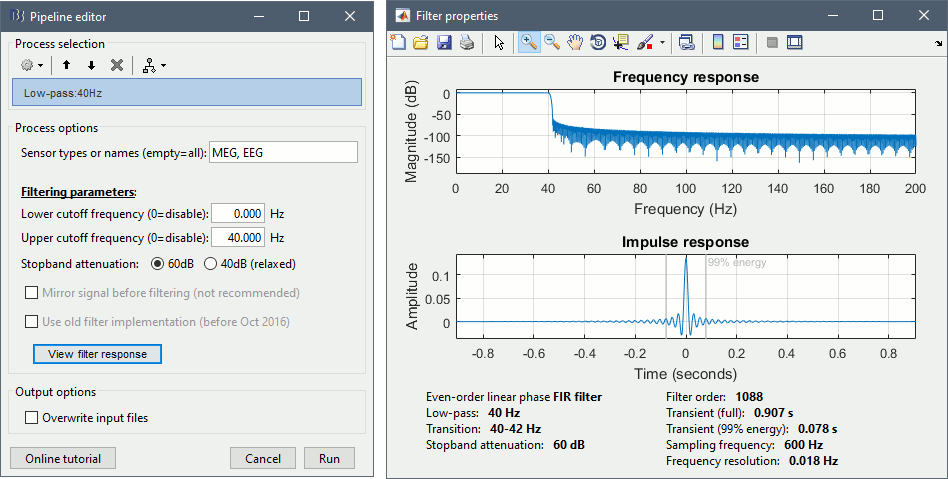
Process options:
Lower cutoff frequency: Defines a high-pass filter (enter 0 for a low-pass filter)
Upper cutoff frequency: Defines a low-pass filter (enter 0 for a high-pass filter)
Stopband attenuation: The higher the attenuation, the higher the performance of the filter, but longer the transient duration. Use the default (60dB) unless you need shorter edge effects.
Use old filter: For replicating results obtained with older versions of Brainstorm.
View filter response: Click on this button to display the impulse and frequency response of your filter, and confirm that the responses appear reasonable.
Filter design:
Description: Even-order linear phase FIR filter, based on a Kaiser window design. The order N is estimated using Matlab's kaiserord function and the filter generated with fir1. Because the filters are linear phase, we can (and do) compensate for the filter delay by shifting the sequence backward in time by M=N/2 samples. This effectively makes the filters zero-phase and zero-delay.
Ripple and attenuation: The allowed ripple in pass and attenuation in stop band are set by default to 10^(-3) and 60dB respectively (note that with Kaiser window design, errors in pass and stopband will always be equal). Transitions between pass and stopbands are set to 15 percent of the upper and lower passband edges. However, when the lower edge of the passband is 5hz or lower we set the transition width to 50 percent of the lower passband edge.
Filtering function: The FIR bandpass filter can be performed in frequency domain (fftfilt function) or in time domain (filter function). The two approaches give the same results, but they have different execution times depending on the filter oder. The time-domain filtering is faster for low-order filters and much slower for high-order filters. The process selects automatically what approach to use.
Edge effects:
Transient (full): With any filtering operation there will always be a transient effect at the beginning of the filtered data. For our filter, this effect will last for half of the filter order: M=N/2 samples. We strongly recommend that your data records are sufficiently long that you can discard these M=N/2 samples. Because we are using zero-phase filtering, there is a similar N/2 effect at the end of the sampled data – these samples should also be discarded.
Transient (99% energy): For some filters, the full transient window might be longer than your epochs. However, most of the energy is carried by the beginning of the filter, and you can obtain amplitudes acceptable for most analysis after a fraction of this full window. For this reason we also mention a much shorter window in the documentation of the filter, which corresponds to the duration needed to obtain 99% of the total energy in the impulse response. This duration corresponds to the "transient" event markers that are added to the recordings when applying filters.

Adjust the parameters: If possible, always discard the full transient window. If the edge effect affects too much of your data, adjust the filter parameters to reduce filter order (increase the lower cut-off frequency or reduce the stopband attenuation). If you cannot get any acceptable compromise, you can consider discarding shorter transient windows, but never go below this "99% energy" window.
Mirroring: We included an option to mirror the data at the start and end of the record instead of padding the signal with zeros. This will reduce the apparent N/2 transients at the start and end of your data record, but you should be aware that these samples are still unreliable and we do not recommend using them.
[TODO] Check this "99% energy" criteria in the case of high-pass filters, it does not seem very useful...
Additional recommendations:
Filter order: The key issue to be aware of when filtering is that the specification you choose for your filter will determine the length of the impulse response (or the filter order) which in turn will affect the fraction of your data that fall into the "edge" region. The most likely factor that will contribute to a high filter order and large edge effects is if you specify a very low frequency at the lower edge of the passband (i.e. the high pass cut-off frequency).
Detrending: If your goal is to remove the DC signal we recommend you first try detrending the data (removes average and best linear fit) to see if this is sufficient. If you still need to remove other low frequency components, then pick the highest cut-off frequency that will fit your needs.
Design optimization: If you are performing bandpass filtering and are not satisfied with the results, you can investigate filtering your data twice, once with a low pass filter and once with a high pass filter. The advantage of this is that you can now separately control the transition widths and stop band attenuation of the two filters. When designing a single BPF using the Kaiser (or any other) window, the maximum deviation from the desired response will be equal in all bands, and the transition widths will be equal at the lower and upper edges of the pass band. By instead using a LPF and a HPF you can optimize each of these processes separately using our filtering function.
Linear phase, no distortion, zero delay: As described earlier, FIR filters have a linear phase in the frequency domain. It means that all samples of the input signal will have a same delay in the output. This delay is compensated after filtering. Consequently, no distortion happens during the filtering process. To illustrate this property, we considered a chirp signal in which the oscillation frequency grows linearly. The signal is band-pass filtered in two frequency ranges. The following plot represents the original signal and its filtered versions with our proposed filters. Results show that the input and output signals of this filter are completely aligned without any delay or distortion.
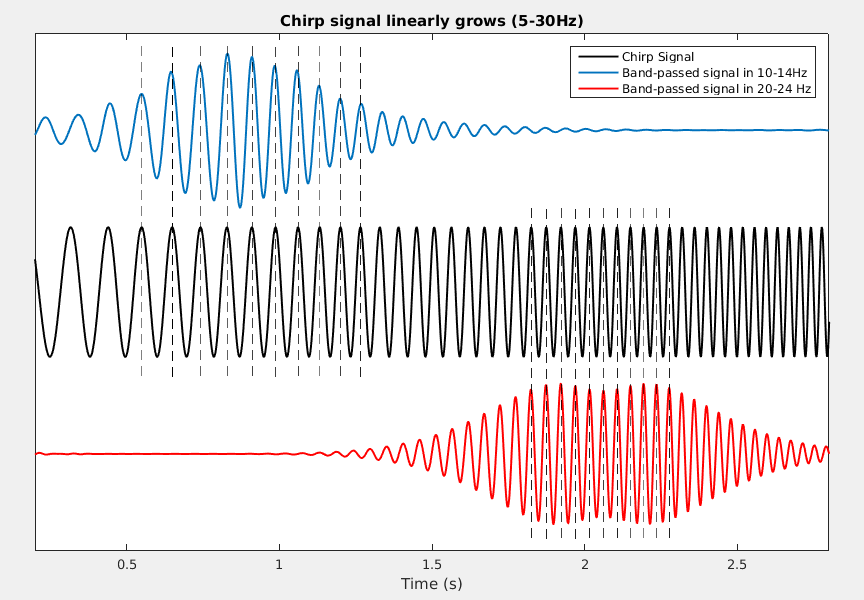
Function: brainstorm3/toolbox/math/bst_bandpass_hfilter.m
External call: process_bandpass('Compute', x, Fs, HighPass, LowPass, 'bst-hfilter', isMirror, isRelax)
Code:
1 function [x, FiltSpec, Messages] = bst_bandpass_hfilter(x, Fs, HighPass, LowPass, isMirror, isRelax, Function, TranBand, Method) 2 % BST_BANDPASS_HFILTER Linear phase FIR bandpass filter. 3 % 4 % USAGE: [x, FiltSpec, Messages] = bst_bandpass_hfilter(x, Fs, HighPass, LowPass, isMirror=0, isRelax=0, Function=[detect], TranBand=[], Method='bst-hfilter-2019') 5 % [~, FiltSpec, Messages] = bst_bandpass_hfilter([], Fs, HighPass, LowPass, isMirror=0, isRelax=0, Function=[detect], TranBand=[], Method='bst-hfilter-2019') 6 % x = bst_bandpass_hfilter(x, Fs, FiltSpec) 7 % 8 % DESCRIPTION: 9 % - A linear phase FIR filter is created. 10 % - Function "kaiserord" and "kaiser" are used to set the necessary order for fir1. 11 % - The transition band can be modified by user. 12 % - Requires Signal Processing Toolbox for the following functions: 13 % kaiserord, kaiser, fir1, fftfilt. If not, using Octave-based alternatives. 14 % 15 % INPUT: 16 % - x : [nChannels,nTime] input signal (empty to only get the filter specs) 17 % - Fs : Sampling frequency 18 % - HighPass : Frequency below this value are filtered in Hz (set to 0 for low-pass filter only) 19 % - LowPass : Frequency above this value are filtered in Hz (set to 0 for high-pass filter only) 20 % - isMirror : isMirror (default = 0 no mirroring) 21 % - isRelax : Change ripple and attenuation coefficients (default=0 no relaxation) 22 % - Function : 'fftfilt', filtering in frequency domain (default) 23 % 'filter', filtering in time domain 24 % If not specified, detects automatically the fastest option based on the filter order 25 % - TranBand : Width of the transition band in Hz 26 % - Method : Version of the filter (2019/2016-18) 27 % 28 % OUTPUT: 29 % - x : Filtered signals 30 % - FiltSpec : Filter specifications (coefficients, length, ...) 31 % - Messages : Warning messages, if any 32 33 % @============================================================================= 34 % This function is part of the Brainstorm software: 35 % https://neuroimage.usc.edu/brainstorm 36 % 37 % Copyright (c) University of Southern California & McGill University 38 % This software is distributed under the terms of the GNU General Public License 39 % as published by the Free Software Foundation. Further details on the GPLv3 40 % license can be found at http://www.gnu.org/copyleft/gpl.html. 41 % 42 % FOR RESEARCH PURPOSES ONLY. THE SOFTWARE IS PROVIDED "AS IS," AND THE 43 % UNIVERSITY OF SOUTHERN CALIFORNIA AND ITS COLLABORATORS DO NOT MAKE ANY 44 % WARRANTY, EXPRESS OR IMPLIED, INCLUDING BUT NOT LIMITED TO WARRANTIES OF 45 % MERCHANTABILITY AND FITNESS FOR A PARTICULAR PURPOSE, NOR DO THEY ASSUME ANY 46 % LIABILITY OR RESPONSIBILITY FOR THE USE OF THIS SOFTWARE. 47 % 48 % For more information type "brainstorm license" at command prompt. 49 % =============================================================================@ 50 % 51 % Authors: Hossein Shahabi, Francois Tadel, John Mosher, Richard Leahy, 52 % 2016-2019 53 54 55 %% ===== PARSE INPUTS ===== 56 % Filter is already computed 57 if (nargin == 3) 58 FiltSpec = HighPass; 59 % Default filter options 60 else 61 if (nargin < 9) || isempty(Method) 62 Method = 'bst-hfilter-2019' ; 63 end 64 if (nargin < 8) || isempty(TranBand) 65 TranBand = []; 66 end 67 if (nargin < 7) || isempty(Function) 68 Function = []; % Auto-detection based on the filter order later in the code 69 end 70 if (nargin < 6) || isempty(isRelax) 71 isRelax = 0; 72 end 73 if (nargin < 5) || isempty(isMirror) 74 isMirror = 0; 75 end 76 FiltSpec = []; 77 end 78 Messages = []; 79 80 81 %% ===== CREATE FILTER ===== 82 if isempty(FiltSpec) 83 % ===== FILTER SPECIFICATIONS ===== 84 Nyquist = Fs/2; 85 % High-pass filter 86 if ~isempty(HighPass) && (HighPass ~= 0) 87 f_highpass = HighPass / Nyquist; % Change frequency from Hz to normalized scale (0-1) 88 switch Method 89 case 'bst-hfilter-2019' 90 if isempty(TranBand) || TranBand==0 91 if (HighPass <= 5) 92 LwTranBand = .5 ; %Hz 93 else 94 LwTranBand = 1 ; %Hz 95 end 96 f_highstop = f_highpass - LwTranBand/Nyquist; 97 else 98 f_highstop = max(0, HighPass - TranBand) / Nyquist; 99 % f_highstop = max(0.2, HighPass - TranBand) / Nyquist; 100 TranBand = (f_highpass - f_highstop)*Nyquist ; % Adjusted Transition band 101 end 102 case 'bst-hfilter-2016' 103 % Default transition band 104 if (HighPass <= 5) % Relax the transition band if HighPass<5 Hz 105 f_highstop = .5 * f_highpass; 106 else 107 f_highstop = .85 * f_highpass; 108 end 109 end 110 else 111 f_highpass = 0; 112 f_highstop = 0; 113 LwTranBand = 1 ; 114 end 115 % Low-pass filter 116 if ~isempty(LowPass) && (LowPass ~= 0) 117 f_lowpass = LowPass / Nyquist; 118 switch Method 119 case 'bst-hfilter-2019' 120 if isempty(TranBand) || TranBand==0 121 UpTranBand = 1 ; 122 UpTranBand = min(UpTranBand,LwTranBand) ; 123 f_lowstop = f_lowpass + UpTranBand/Nyquist; 124 else 125 f_lowstop = f_lowpass + TranBand/Nyquist; 126 end 127 case 'bst-hfilter-2016' 128 % Default transition band 129 if f_highpass==0 % If this is a low-pass filter 130 f_lowstop = 1.05 * f_lowpass; 131 else 132 f_lowstop = 1.15 * f_lowpass; 133 end 134 end 135 else 136 f_lowpass = 0; 137 f_lowstop = 0; 138 end 139 % If both high-pass and low-pass are zero 140 if (f_highpass == 0) && (f_lowpass == 0) 141 Messages = ['No frequency band in input.' 10]; 142 return; 143 % Input frequencies are too high 144 elseif (f_highpass >= 1) || (f_lowpass >= 1) 145 Messages = sprintf('Cannot filter above %dHz.\n', Nyquist); 146 return; 147 end 148 % Transition parameters 149 if isRelax 150 Ripple = 10^(-2); 151 Atten = 10^(-2); % Equals 40db 152 else 153 Ripple = 10^(-3); % pass band ripple 154 Atten = 10^(-3); % Equals 60db 155 end 156 157 % ===== DESIGN FILTER ===== 158 % Build the general case first 159 fcuts = [f_highstop, f_highpass, f_lowpass, f_lowstop]; 160 mags = [0 1 0]; % filter magnitudes 161 devs = [Atten Ripple Atten]; % deviations 162 % Now adjust for desired properties 163 fcuts = max(0,fcuts); % Can't go below zero 164 fcuts = min(1-eps, fcuts); % Can't go above or equal to 1 165 166 % We have implicitly created a bandpass, but now adjust for desired filter 167 if (f_lowpass == 0) % User didn't want a lowpass 168 fcuts(3:4) = []; 169 mags(3) = []; 170 devs(3) = []; 171 end 172 if (f_highpass == 0) % User didn't want a highpass 173 fcuts(1:2) = []; 174 mags(1) = []; 175 devs(1) = []; 176 end 177 178 % Generate FIR filter 179 % Using Matlab's Signal Processing toolbox 180 if bst_get('UseSigProcToolbox') 181 [n,Wn,beta,ftype] = kaiserord(fcuts, mags, devs, 2); 182 n = n + rem(n,2); % ensure even order 183 b = fir1(n, Wn, ftype, kaiser(n+1,beta), 'noscale'); 184 % Using Octave-based functions 185 else 186 [n,Wn,beta,ftype] = oc_kaiserord(fcuts, mags, devs, 2); 187 n = n + rem(n,2); % ensure even order 188 b = oc_fir1(n, Wn, ftype, oc_kaiser(n+1,beta), 'noscale'); 189 end 190 191 % Filtering function: Detect the fastest option, if not explicitely defined 192 if isempty(Function) 193 % The filter() function is a bit faster for low-order filters, but much slower for high-order filters 194 if (n > 800) % Empirical threshold 195 Function = 'fftfilt'; 196 else 197 Function = 'filter'; 198 end 199 end 200 201 % Compute the cumulative energy of the impulse response 202 E = b((n/2)+1:end) .^ 2 ; 203 E = cumsum(E) ; 204 E = E ./ max(E) ; 205 % Compute the effective transient: Number of samples necessary for having 99% of the impulse response energy 206 [tmp, iE99] = min(abs(E - 0.99)) ; 207 208 % Output structure 209 FiltSpec.b = b; 210 FiltSpec.a = 1; 211 FiltSpec.order = n; 212 FiltSpec.transient = iE99 / Fs ; % Start up and end transients in seconds (Effective) 213 % FiltSpec.transient_full = n / (2*Fs) ; % Start up and end transients in seconds (Actual) 214 FiltSpec.f_highpass = f_highpass; 215 FiltSpec.f_lowpass = f_lowpass; 216 FiltSpec.fcuts = fcuts * Nyquist ; % Stop and pass bands in Hz (instead of normalized) 217 FiltSpec.function = Function; 218 FiltSpec.mirror = isMirror; 219 % If empty input: just return the filter specs 220 if isempty(x) 221 return; 222 end 223 end 224 225 %% ===== FILTER SIGNALS ===== 226 % Transpose signal: [time,channels] 227 [nChan, nTime] = size(x); 228 % Half of filter length 229 M = FiltSpec.order / 2; 230 % If filter length > 10% of data length 231 edgePercent = 2*FiltSpec.transient / (nTime / Fs); 232 if (edgePercent > 0.1) 233 Messages = [Messages, sprintf('Start up and end transients (%.2fs) represent %.1f%% of your data.\n', 2*FiltSpec.transient, 100*edgePercent)]; 234 end 235 236 % Remove the mean of the data before filtering 237 xmean = mean(x,2); 238 x = bst_bsxfun(@minus, x, xmean); 239 240 % Mirroring requires the data to be longer than the filter 241 if (FiltSpec.mirror) && (nTime < M) 242 Messages = [Messages, 'Warning: Data is too short for mirroring. Option is ignored...' 10]; 243 FiltSpec.mirror = 0; 244 end 245 % Mirror signals 246 if (FiltSpec.mirror) 247 x = [fliplr(x(:,1:M)), x, fliplr(x(:,end-M+1:end))]; 248 % Zero-padding 249 else 250 x = [zeros(nChan,M), x, zeros(nChan,M)] ; 251 end 252 253 % Filter signals 254 switch (FiltSpec.function) 255 case 'fftfilt' 256 if bst_get('UseSigProcToolbox') 257 x = fftfilt(FiltSpec.b, x')'; 258 else 259 x = oc_fftfilt(FiltSpec.b, x')'; 260 end 261 case 'filter' 262 x = filter(FiltSpec.b, FiltSpec.a, x, [], 2); 263 end 264 265 % Remove extra data 266 x = x(:,2*M+1:end); 267 % Restore the mean of the signal (only if there is no high-pass filter) 268 if (FiltSpec.f_highpass == 0) 269 x = bst_bsxfun(@plus, x, xmean); 270 end
Filter specifications: Notch
Description: 2nd order IIR notch filter with zero-phase lag (implemented with filtfilt).
Reference: Mitra, Sanjit Kumar, and Yonghong Kuo. Digital signal processing: a computer-based approach. Vol. 2. New York: McGraw-Hill, 2006. MatlabCentral #292960
Edge effects: It is computed based on the 99% energy of the estimated impulse response.
Function: brainstorm3/toolbox/process/functions/process_notch.m
External call: [x, FiltSpec, Messages] = Compute(x, sfreq, FreqList, Method, bandWidth)
Filter specifications: Band-stop
Description: 4th order Butterworth IIR filter with zero-phase lag (implemented with filtfilt)
Reference: FieldTrip: x = ft_preproc_bandstopfilter(x, sfreq, FreqBand, [], 'but', 'twopass')
Edge effects It is computed based on the 99% energy of the estimated impulse response.
Function: brainstorm3/toolbox/process/functions/process_bandstop.m
External call: x = process_bandstop('Compute', x, sfreq, FreqList, FreqWidth)
On the hard drive
The names of the files generated by the process "Power spectrum density" start with the tag timefreq_psd, they share the same structure as all the files that include a frequency dimension.
To explore the contents of a PSD file created in this tutorial, right-click on it and use the popup menus
File > View file contents or File > Export to Matlab.
Structure of the time-frequency files: timefreq_psd_*.mat
TF: [Nsignals x Ntime x Nfreq] Stores the spectrum information. Nsignals is the number of channels that were selected with the option "MEG" in the PSD process. Nfreq is the number of frequency bins. There is no time dimension (Ntime = 1).
Comment: String used to represent the file in the database explorer.
Time: Window of time over which the file was estimated.
TimeBands: Defined only when you select the option "Group in time bands".
Always empty for the PSD files because there is no time dimension.Freqs: [1 x Nfreq] List of frequencies for which the power spectrum was estimated (in Hz).
RefRowNames: Only used for connectivity results.
RowNames: [Nsignals x 1] Describes the rows of the TF matrix (first dimension). Here it corresponds to the name of the MEG sensors, in the same order as is the .TF field.
Measure: Function currently applied to the FFT coefficients {power, none, magnitude, log, other}
Method: Function that was used to produce this file {psd, hilbert, morlet, corr, cohere, ...}
DataFile: File from which this file was calculated = Parent file in the database explorer.
DataType: Type of file from which this file was calculated (file type of .DataFile).
- 'data' = Recordings
- 'cluster' = Recordings grouped by clusters of sensors
- 'results' = Source activations
- 'scouts' = Time series associated with a region of interest
SurfaceFile / GridLoc / GridAtlas / Atlas: Used only when the input file was a source file.
Leff: Effective number of averages = Number of input files averaged to produce this file.
Options: Most relevant options that were passed to the function bst_timefreq.
History: Describes all the operations that were performed with Brainstorm on this file. To get a better view of this piece of information, use the menu File > View file history.
Useful functions
in_bst_timefreq(PsdFile): Read a PSD or time-frequency file.
in_bst(FileName): Read any Brainstorm file.
bst_process('LoadInputFile', FileName, Target): The most high-level function for reading Brainstorm files. "Target" is a string with the list of sensor names or types to load (field RowNames).
bst_psd(F, sfreq, WinLength, WinOverlap): Computation of the Welch's power spectrum density.
Additional documentation
Forum discussions
Tutorial 11: Bad channels
Authors: Francois Tadel, Elizabeth Bock, Sylvain Baillet
It is common during the acquisition to have a few sensors that are recording values that will not be usable in the data analysis. In MEG, a sensor can be damaged or unstable. In EEG, the quality of the connection between the electrode and the scalp is sometimes too low to record anything interesting.
It is important to identify the sensors with poor signal quality at an early stage of the pre-processing, because the efficiency of the artifact removal will depend on it. If you try to remove blink and cardiac artifacts with some bad sensors it may not work very well, and worse, it will propagate the bad signals to all the channels.
This tutorial will explain the various ways we have to handle the bad channels. Note that the recordings from this auditory experiment do not contain any bad sensors, therefore the entire tutorial is optional. If you are not interested, you can skip it and will still be able to follow the next tutorials.
Contents
Identifying bad channels
Some bad channels are easy to detect, their signals look either completely off or totally flat compared with the other surrounding sensors. Some others are more difficult to identify. The examples below are taken from other datasets.
The power spectrum density (PSD) is usually a good way to spot a few bad channels, this is why we always recommend to compute it for all the datasets:
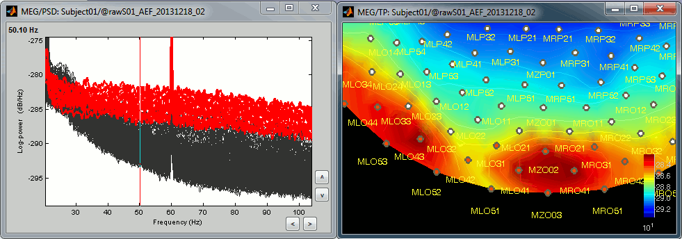
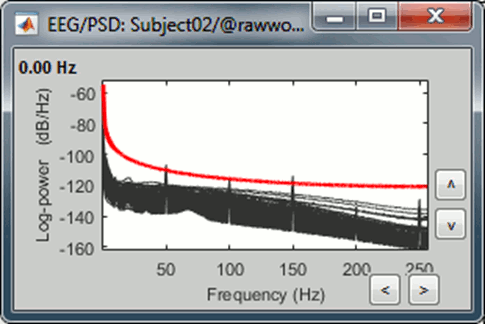
Simply looking at the signals traces, some channels may appear generally noisier than the others:
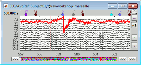
Looking at a 2D sensor topography, if one sensor shows very different values from its neighbors for extended periods of time, you can doubt of its quality:
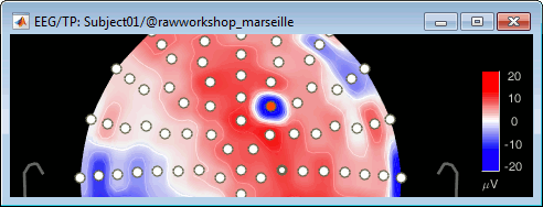
Selecting sensors
- Double-click on the recordings for run #01 to open the MEG sensors.
Right-click on the time series figure > View topography (or press Ctrl+T).
Right-click on the topography figure > Channels > Display sensors (or press Ctrl+E).
If you can't see anything because the topography figure is too small, you can change the way the figures are automatically arranged. In the top-right corner of the Brainstorm figure, select the menu "Window layout options > Tiled".
You can select one channel by clicking on its signal or on the dot representing it in the topography figure. Note that the sensor selection is automatically reported to the other figure.
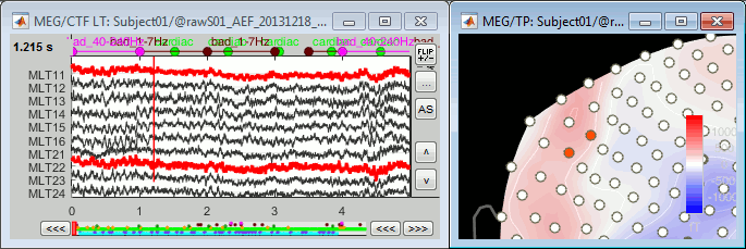
You can select multiple sensors at the same time the topography figure.
Right-click on the figure, then hold the mouse button and move the mouse.
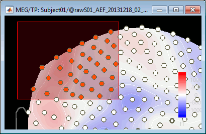
Select a few sensors, then right-click on one of the figures and check out the Channels menu:
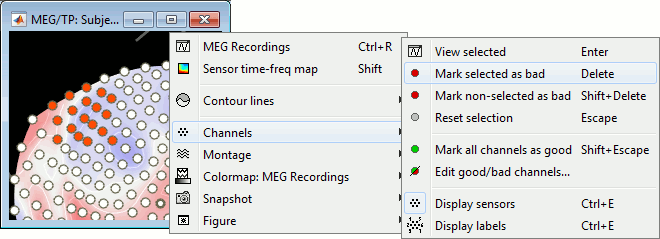
View selected: Show the time series of the selected sensors.
Mark selected as bad: Remove sensors from the display and all the further computations.
Mark non-selected as bad: Keep only the selected channels.
Reset selection: Unselect all the selected sensors.
Mark all channels as good: Brings back all the channels to display.
Edit good/bad channels: Opens an interface that looks like the channel editor, but with one extra column to edit the status (good or bad) of each channel.
Marking bad channels
Select a few channels, right-click > Channels > Mark selected as bad (or press the Delete key).
The selected channels disappear from the two views. In the time series figure, the signals are not visible anymore, in the topography the corresponding dots disappear and the values of the magnetic fields around the missing sensors get re-interpolated based on what is left.
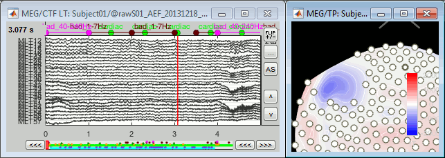
With the time series figure, you can display the signals that have been tagged as bad.
In the Record tab, select the montage "Bad channels".
In this view, you cannot select the channels, they are not available anymore.

Right-click on a figure > Channels > Edit good/bad channels.
This menu open a window very similar to the Channel Editor window, with additional green and red dots to indicate the status of each channel. Click on the dot to switch it to good or bad.

From the database explorer
Many options to change the list of bad channels are available from the database explorer.
The menus are available if you right-click one data file (or link to raw file). In this case, the selected operation is applied only on the selected file.

The same menus are also available for all the folders. In this case, the selected operation is applied recursively to all the data files (and links to raw files) that are found in the folder.

With this batching ability of the database explorer, you can quickly tag some bad channels in all the recordings of a subject or for the entire protocol. You can also get a quick overview of all the bad channels in all the files at once with the menu View all bad channels.

Restore all the good channels before moving to the next tutorial. For instance, right-click on the protocol folder TutorialIntroduction > Good/bad channels > Mark all channels as good.
Epoching and averaging
The list of bad channels is saved separately for each dataset.
At this stage of the analysis, the database contains only links to continuous files. When you import epochs from a continuous file, the list of bad channels will be copied from the raw file to all the imported data files.
Then you will be able to redefine this list for each epoch individually, tagging more channels as bad, or including back the ones that are ok. This way it is possible to exclude from the analysis the channels that are too noisy in a few trials only, for instance because of some movement artifacts.
When averaging, if an epoch contains one bad channel, this bad channel is excluded from the average but all the other channels are kept. If the same channel is good in other trials, it will be considered as good in the average. This means that not all the channels have the same number of trials for calculating the average.
This may cause the different channels of an averaged file to have different signal-to-noise ratios, which may lead to confusing results. However, we decided to implement the average in this way to be able to keep more data in the studies with a low number of trials and a lot of noise.
On the hard drive
The list of bad channels is saved for each data file separately, in the field ChannelFlag.
This vector indicates for each channel #i if it is good (ChannelFlag(i)= 1) or bad (ChannelFlag(i)= -1).
Right-click on a link to a continuous file > File > View file contents:
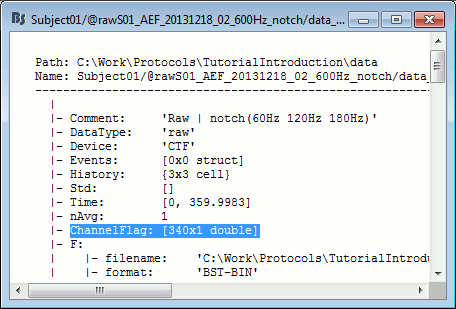
For raw data files, this information is duplicated in the sFile structure (F field) in order to be passed easily to the low-level reading functions. If you are planning to modify the list of bad channels manually, you need to change two fields: mat.ChannelFlag and mat.F.channelflag. For imported data, you just need to modify the field mat.ChannelFlag.
Tutorial 12: Artifact detection
Authors: Francois Tadel, Elizabeth Bock, Sylvain Baillet
The previous tutorials illustrated how to remove noise patterns occurring continuously and at specific frequencies. However, most of the events that contaminate the MEG/EEG recordings are not persistent, span over a large frequency range or overlap with the frequencies of the brain signals of interest. Frequency filters are not appropriate to correct for eye movements, breathing movements, heartbeats or other muscle activity.
For getting rid of reproducible artifacts, one popular approach is the Signal-Space Projection (SSP). This method is based on the spatial decomposition of the MEG/EEG recordings for a selection of time samples during which the artifact is present. Therefore we need to identify when each type of artifacts occurs in the recordings. This tutorial shows how to automatically detect some well defined artifacts: the blinks and the heartbeats.
Contents
Observation
Let's start by observing the type of contamination the blinks and heartbeats cause to the MEG recordings.
Run #01: Double-click on the link to show the MEG sensors.
Configuration: Page of 3 seconds, view in columns, selection of the "CTF LT" sensors (the left-temporal sensors will be a good example to show at the same time the two types of artifacts).
EOG: Right-click on the link > EOG > Display time series. Two channels are classified as EOG:
VEOG: Vertical electrooculogram (two electrodes placed below and above one eye)
HEOG: Horizontal electrooculogram (two electrodes placed on the temples of the subject)
- On these traces, there is not much happening for most of the recordings except for a few bumps. This subject is sitting very still and not blinking much. We can expect MEG recordings of a very good quality.
ECG: Right-click on the link > ECG > Display time series.
The electrocardiogram was recorded with a bipolar montage of electrodes across the chest. You can recognize the typical shape of the electric activity of the heart (P, QRS and T waves).Find a blink: Scroll through the recordings using the F3 shortcut until you see a large blink.
- Remember you can change the amplitude scale with many shortcuts (eg. right-click + move).
To keep the scale fixed between two pages: Uncheck the button [AS] (auto-scale).
- For instance, you can observe a nice blink at 20.8s (red cursor in the screen capture below).
- On the same page, you should be able to observe the contamination due to a few heartbeats, corresponding to the peaks of the ECG signal (eg. 19.8s, shown as a blue selection below).
The additional data channels (ECG and EOG) contain precious information that we can use for the automatic detection of the blinks and heartbeats. We strongly recommend that you always record these signals during your own experiments, it helps a lot with the data pre-processing.
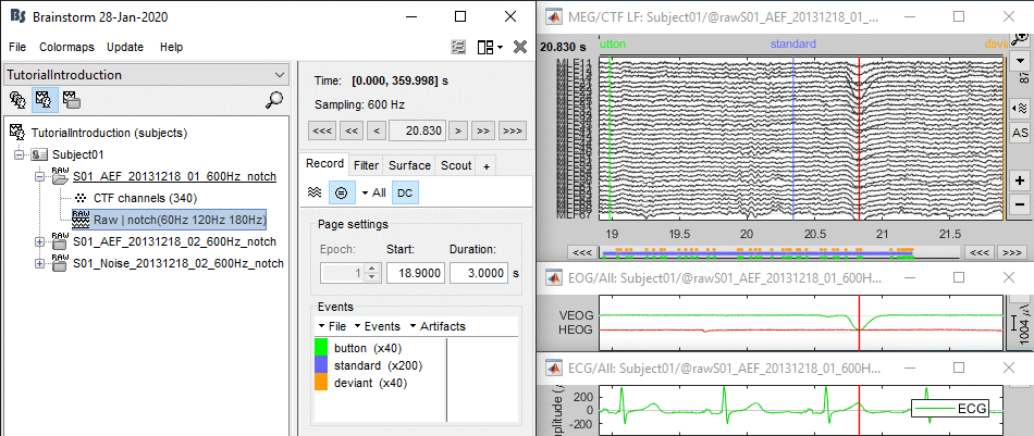
Detection: Heartbeats
In the Record tab, select the menu: "Artifacts > Detect heartbeats".
- It automatically opens the pipeline editor, with the process "Detect heartbeats" selected.
Channel name: Name of the channel that is used to perform the detection. Select or type "ECG".
Time window: Time range that the algorithm should scan for amplitude peaks. Leave the default values to process the entire file, or check the option [All file].
Event name: Name of the event group created for saving the detected events. Enter "cardiac".
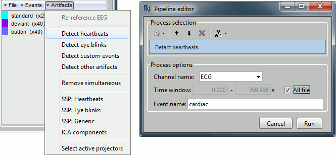
Click on Run. After the process stops, you can see a new event category "cardiac". The 464 (aprox.) heartbeats for 360s of recordings indicate an average heart rate of 77bpm, everything looks normal.
You can check a few of them, to make sure the "cardiac" markers really indicate the ECG peaks. Not all peaks need to be detected, but you should have a minimum of 10-20 events marked for removing the artifacts using SSP, described in the following tutorials.

Detection: Blinks
Now do the same thing for the blinks: Menu "Artifacts > Detect eye blinks".
Channel name: VEOG
Time window: All file
Event name: Blink
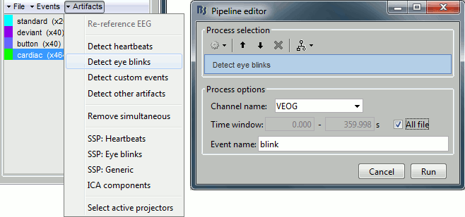
Run, then look quickly at the 15 detected blinks (shortcut: Shift+Right arrow).

Remove simultaneous blinks/heartbeats
We will use these event markers as the input to our SSP cleaning method. This technique works well if each artifact is defined precisely and as independently as possible from the other artifacts. This means that we should try to avoid having two different artifacts marked at the same time.
Because the heart beats every second or so, there is a high chance that when the subject blinks there is a heartbeat not too far away in the recordings. We cannot remove all the blinks that are contaminated with a heartbeat because we would have no data left. But we have a lot of heartbeats, so we can do the contrary: remove the markers "cardiac" that are occurring during a blink.
In the Record tab, select the menu "Artifacts > Remove simultaneous". Set the options:
Remove events named: "cardiac"
When too close to events: "blink"
Minimum delay between events: 250ms
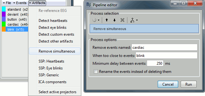
After executing this process, the number of "cardiac" events goes from 465 to 456. The deleted heartbeats were all less than 250ms away from a blink.
Run #02: Running from a script
Let's perform the same detection operations on Run #02, using this time the Process1 box.
Close everything with the [X] button at the top-right corner of the Brainstorm window.
Select the run AEF #02 in the Process1 box, then select the following processes:
Events > Detect heartbeats: Select channel ECG, check "All file", event name "cardiac".
Events > Detect eye blinks: Select channel VEOG, check "All file", event name "blink".
Events > Remove simultaneous: Remove "cardiac", too close to "blink", delay 250ms.
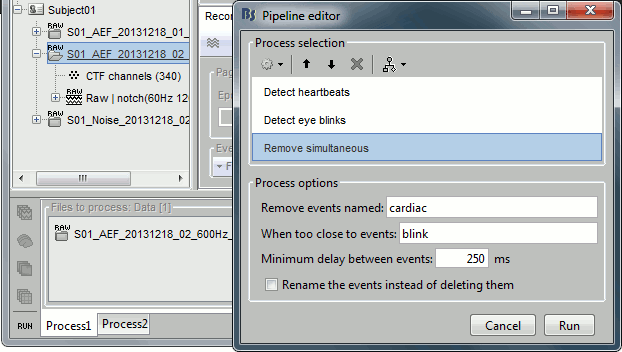
Open the Run#02 recordings (MEG+EOG+ECG) and verify that the detection worked as expected. You should get 472 cardiac events and 19 blink events.
Artifacts classification
If the EOG signals are not as clean as here, the detection processes may create more than one category, for instance: blink, blink2, blink3. The algorithm not only detects specific events in a signal, it also classifies them by shape. For two detected events, the signals around the event marker have to be sufficiently correlated (> 0.8) to be classified in the same category. At the end of the process, all the categories that contain less than 5 events are deleted.
In the good cases, this can provide an automatic classification of different types of artifacts, for instance: blinks, saccades and other eye movements. The tutorial MEG median nerve (CTF) is a good illustration of appropriate classification: blink groups the real blinks, and blink2 contains mostly saccades.
In the bad cases, the signal is too noisy and the classfication fails. It leads to either many different categories, or none if all the categories have less than 5 events. If you don't get good results with the process "Detect eye blinks", you can try to run a custom detection with the classification disabled.
At the contrary, if you obtain one category that mixes multiple types of artifacts and would like to automatically separate them in different sub-groups, you can try the process "Events > Classify by shape". It is more powerful than the automatic classification from the event detection process because it can run on multiple signals at the same type: first it reduces the number of dimensions with a PCA decomposition, then runs a similar classification procedure.
Detection: Custom events
These two processes "Detect heartbeats" and "Detect eye blinks" are in reality shortcuts for a generic process "Detect custom events". This process can be used for detecting any kind of event based on the signal power in a specific frequency band. We are not going to use it here, but you may have to use it if the standard parameters do not work well, or for detecting other types of events.
- The signal to analyze is read from the continuous file (options "Channel name" and "Time window").
Frequency band: The signal is filtered in a frequency band where the artifact is easy to detect. For EOG: 1.5-15Hz ; for ECG: 10-40Hz.
Threshold: An event of interest is detected if the absolute value of the filtered signal value goes over a given number of times the standard deviation. For EOG: 2xStd, for ECG: 4xStd
Minimum duration between two events: If the filtered signal crosses the threshold several times in relation with the same artifact (eg. muscle activity in an EMG channel), we don't want to trigger several events but just one at the beginning of the activity. This parameter would indicate the algorithm to take only the maximum value over the given time window; it also prevents from detecting other events immediately after a successful detection. For the ECG, this value is set to 500ms, because it is very unlikely that the heart rate of the subject goes over 120 beats per minute.
Ignore the noisy segments: If this option is selected, the detection is not performed on the segments that are much noisier than the rest of the recordings.
Enable classification: If this option is selected, the events are classified by shape in different categories, based on correlation measure. In the end, only the categories that have more than 5 occurrences are kept, all the other successful detections are ignored.
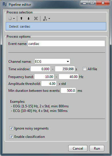
In case of failure
If the signals are not as clean as in this sample dataset, the automatic detection of the heartbeats and blinks may fail with the standard parameters. You may have to use the process "Detect custom events" and adjust some parameters. For instance:
- If nothing is detected: decrease the amplitude threshold, or try to adjust the frequency band.
- If too many events are detected: increase the amplitude threshold or the minimum duration between two events.
- If too many categories of events are generated, and you have a very little number of events in the end: disable the classification.
- To find the optimal frequency band for an artifact, you can open the recordings and play with the online band-pass filters in the Filter tab. Keep the band that shows the highest amplitude peaks.
If you cannot get your artifacts to be detected automatically, you can browse through the recordings and mark all the artifacts manually, as explained in the tutorial Event markers..
Other detection processes
Events > Detect analog trigger
See tutorial Stimulation delays.
This is used to detect events on any channel (MEG, EEG, STIM, Analog, etc), where the baseline is relatively stable and the events will predictably cross a threshold. This is useful when you want to detect a single time point (simple event) at the start of an event, as in these examples:
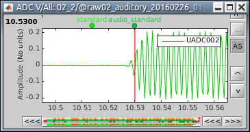
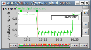
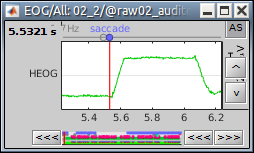
Events > Detect custom events
See tutorial Artifact detection.
This is used to detect events on any channel (MEG, EEG, STIM, Analog, etc) where the baseline is relatively stable and the events will predictably cross a threshold. This is useful when you want to detect a simple event at the peak of an event, as in these examples:
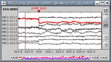
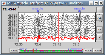
Events > Detect events above threshold
See tutorial MEG visual: single subject.
This is used to detect signal on any channel (MEG, EEG, STIM, Analog, etc) that is above a defined threshold value. This is useful when you want to detect all time points when the signal is above the threshold (extended events), as in these examples:
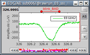
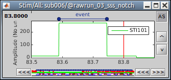
The extended event can be converted to a single event (when the rising or falling edge is desired). in the Record tab, select the event to convert, then in the menu Events > Convert to simple event > select Start, Middle, or End to indicate where the marker should be placed.
Events > Detect other artifacts
See tutorial Additional bad segments
Events > Detect movement
See tutorial Detect subject movements
Synchronize > Transfer events
See tutorial Synchronization with eye tracker
Artifacts > Detect bad channels: Peak-to-peak
With imported data: Reject channels and trials from imported data.
With raw data: Create bad events (specific channel or all channels) on the raw data.
- This process is usually not recommended, as the amplitude of the signal is not always a good marker of the quality of the channel.
Artifacts > Detect bad: amplitude and gradient thresholds
With imported data: Reject trials from imported data.
With raw data: Create bad events (all channels) on the raw data. Data is analyzed in windows which length is defined by the user.
This process detects artifactual segments for MEG recordings based on the distribution of the signal peak-to-peak amplitude and the signal numerical gradient. This process is based on the AUTO option of the MEG trial rejection method available in ArtifactScanTool.
Segments are identified as artifactual if they surpass the specified thresholds. These thresholds can be set in two ways: auto, thresholds are defined as n times the median absolute deviations (MAD) of each signal characteristic; manual: user provides the thresholds. Once the process is executed, the report shows the distribution and thresholds for the two signal characteristics.
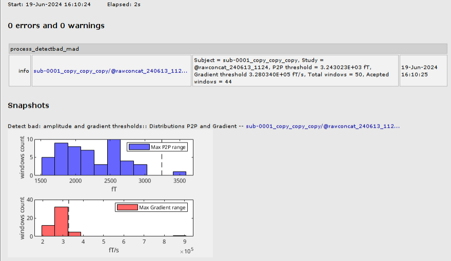
Additional documentation
Tutorial: Detect subject movements
Tutorial: Synchronization with eye tracker
Tutorial 13: Artifact cleaning with SSP
Authors: Francois Tadel, Elizabeth Bock, John C Mosher, Sylvain Baillet
As previously said, the frequency filters are not adapted to remove artifacts that are transient or overlapping in frequency domain with the brain signals of interest. Other approaches exist to correct for these artifacts, based on the spatial signature of the artifacts.
If an event is very reproducible and occurs always at the same location (eg. eye blinks and heartbeats), the sensors will always record the same values when it occurs. We can identify the topographies corresponding to this artifact (ie. the spatial distributions of values at one time point) and remove them from the recordings. This spatial decomposition is the basic idea behind two widely used approaches: the SSP (Signal-Space Projection) and ICA (Independent Component Analysis) methods.
This introduction tutorial will focus on the SSP approach, as it is a lot simpler and faster but still very efficient for removing blinks and heartbeats from MEG recordings. For cleaning EEG data, ICA is ofter better indicated - the interface for running ICA decompositions is very similar and is described in an advanced tutorial.
Contents
Overview
The general SSP objective is to identify the sensor topographies that are typical of a specific artifact, then to create spatial projectors to remove the contributions of these topographies from the recordings.
- We start by identifying many examples of the artifact we are trying to remove. This is what we've been doing in the previous tutorial with the creation of the "cardiac" and "blink" events.
- We extract a short time window around each of these event markers and concatenate in time all the small blocks of recordings.
- We run a principle components analysis (PCA) on the concatenated artifacts in order to get a decomposition in various spatial components (number of components = number of sensors).
- If it works well, we can find in the first few principal components some topographies that are very specific of the type of artifact we are targeting. We select these components to remove.
- We compute a linear projector for each spatial component to remove and save them in the database (in the "Link to raw file"). They are not immediately applied to the recordings.
- Whenever some recordings are read from this file, the SSP projectors are applied on the fly to remove the artifact contributions. This approach is fast and memory efficient.
Note that these tools are available on continuous files only ("Link to raw file") and cannot be applied to recordings that have already been imported in the database.
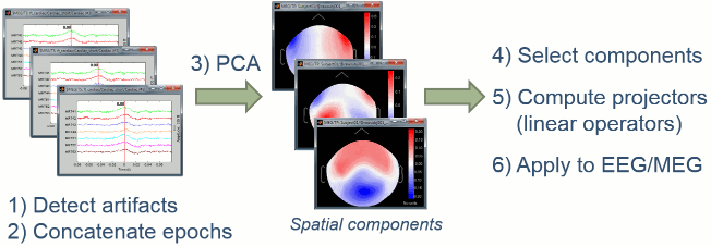
The order matters
This procedure has to be repeated separately for each artifact type. The order in which you process the artifacts matters, because for removing the second artifact we typically use the recordings cleaned with the first set of SSP projectors. We have to decide which one to process first.
It works best if each artifact is defined precisely and as independently as possible from the other artifacts. If the two artifacts happen simultaneously, the SSP projectors calculated for the blink may contain some of the heartbeat topography and vice versa. When trying to remove the second artifact, we might not be able to clearly isolate it anymore.
Because the heart beats every second or so, there is a high chance that when the subject blinks there is a heartbeat not too far away in the recordings. Therefore a significant number of the blinks will be contaminated with heartbeats. But we have usually a lot of "clean" heartbeats, we can start by removing these ones. To correctly isolate these two common artifacts, we recommend the following procedure:
- Remove the markers "cardiac" that are occurring during a blink (done in the previous tutorial),
Compute the cardiac SSP (with no eye movements, because we removed the co-occurring events),
Compute the blink SSP (with no heartbeats, because they've already been taken care of).
If you have multiple modalities recorded simultaneously, for example MEG and EEG, you should run this entire procedure twice, once for the EEG only and once for the MEG only. You will always get better results if you process the different types of sensors separately. Same thing when processing Elekta-Neuromag recordings: separately process the magnetometers (MEG MAG) and the gradiometers (MEG GRAD).
SSP: Heartbeats
Double-click on the link to show the MEG sensors for Run #01.
In the Record tab, select the menu: "Artifacts > SSP: Heartbeats".
Event name: Name of the event to use to calculate the projectors, enter "cardiac".
Sensor types: Type of sensors for which the projection should be calculated ("MEG"). Note that you will always get better results if you process the different types of sensors separately.
Compute using existing SSP projectors: You have the option to calculate the projectors from the raw recordings, or from the recordings filtered with the previously computed SSP projectors.
Unless you have a good reason for not considering the existing projectors, you should select this option. Then if the results are not satisfying, try again with the option disabled.
For this step it doesn't make any difference because there are not projectors yet in the file.
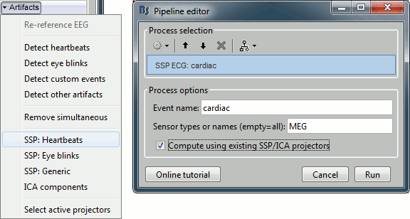
After the computation is done, a new figure is displayed, that lets you select the active projectors.
On the left: The projector categories where each row represents the result of an execution of this process (usually one for each sensor type and each artifact).
On the right: The spatial components returned by the PCA decomposition. The percentage indicated between brackets is the singular value for this each component, normalized for this decomposition (percentage = Si / sum(Si), see technical details at the end of this page).
Percentage: More practically, it indicates the amount of signal that was captured by the component during the decomposition. The higher it is, the more the component is representative of the artifact recordings that were used to calculate it. In the good cases, you would typically see one to three components with values that are significantly higher than the others.
- When a component is selected, it means that it is removed from the recordings. A spatial projector is computed and applied to the recordings on the fly when reading from the continuous file.
Default selection: The software selects the first component and leaves the others unselected. This selection is arbitrary and doesn't mean the cleaning is correct, you should always manually review the components that you want to remove.
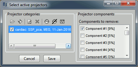
Evaluate the components
The percentage indicated for the first value (9%) is much higher than the following ones (5%, 5%, 4%, 3%...), this could indicate that it targets relatively well the cardiac artifact. Let's investigate this.
Click on the first component, then click on the toolbar button [Display component topography]. This menu shows the spatial distribution of the sensor values for this component. Note that you don't have to select the component (ie. check the box) to display it. This topography seems to correspond to a strong dipolar activity located relatively far from the sensor array, it matches the type of artifact we expect from the heart activity.

The second button "Display component topography [No magnetic interpolation]" produces the same figure but without the reinterpolation of the magnetic fields that is typically applied to the MEG recordings in Brainstorm, it may help understand some difficult cases. This magnetic interpolation will be detailed later in the introduction tutorials.
You can display multiple components in the same figure: select them at the same time in the list (holding the Shift/Ctrl/Cmd button of your keyboard) and then click on the button "Display topography". No other strong components looks like it could be related with the heartbeats.
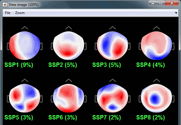
The last button in the toolbar [Display component time series], opens a figure that represents the evolution of the contribution of this component over time. The higher the amplitude, the more present the selected topography in the recordings. Click on it to show the component #1, then display the ECG signal at the same time (right-click on the file > ECG > Display time series).
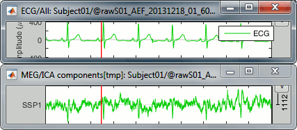
We observe that the "SSP1" trace correlates relatively well with the ECG trace, in the sense that we captured most the ECG peaks with this component. However, the component seems also to capture much more signal than just the heartbeats: many alpha oscillations and some of the ocular activity. The example below shows a blink in the EOG, ECG and SSP component #1.
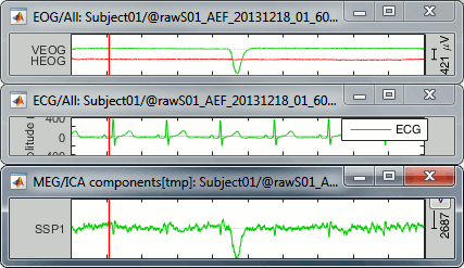
If you remove this component from the recordings, you can expect to see most of the artifacts related with the cardiac activity to go away, but you will also remove additional signal elements that were not really well identified. The job is done but it causes some unwanted side effects.
- It is in general possible to refine the SSP decomposition by going back to the selection of "cardiac" markers that we used to compute it. You could look at all the ECG peaks individually and remove the markers located in segments of recordings that are noisier or that contain a lot of alpha activity (~10Hz). You would need to delete this SSP decomposition and run again the same process.
Alternatively, or if you don't manage to extract a clean cardiac component with a PCA/SSP decomposition, you could try to run an ICA decomposition instead. You might be able to get better results, but it comes with significant computation and manual exploration times. Note that for some subjects, the cardiac artifact is not very strong and could be simply ignored in the analysis.
Evaluate the correction
The topography of the component #1 looks like it represents the heart activity and its temporal evolution shows peaks where we identified heartbeats. It is therefore a good candidate for removal, we just need to make sure the signals look good after the correction before validating this choice.
- Show the left-temporal MEG sensors (CTF LT) and select/unselect the first SSP component.
- Repeat this for different time windows, to make sure that the cardiac peaks in the MEG sensors really disappear when the projector #1 is selected and that the rest is not altered too much.
No correction:
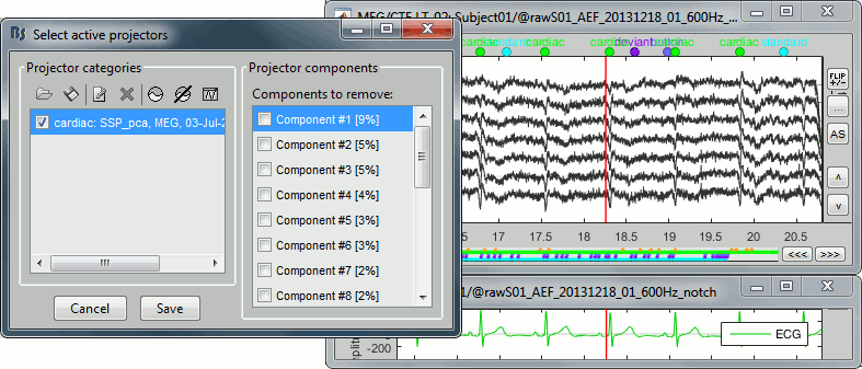
Cardiac component #1 removed:
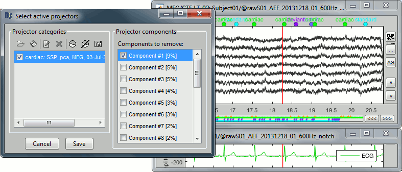
In this example we will consider that the current decomposition is good enough.
Make sure you select the component #1, then click on [Save] to validate the modifications.After this window is closed, you can always open it again from the Record tab with the menu Artifacts > Select active projectors. At this stage of the analysis, you can modify the list of projectors applied to the recordings at any time.
SSP: Eye blinks
Let's try the same thing with the eye blinks.
Select the process "Artifacts > SSP: Eye blinks"
Run it on the event type "blink", that indicates the peaks of the VEOG signal.
Select the option "Compute using existing projectors" (if this step doesn't seem to work correctly, try again without selecting this option).
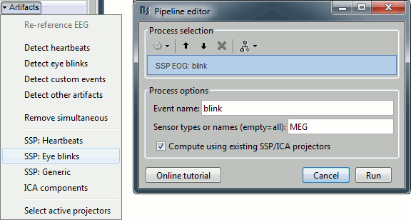
You see now a new category of projectors. Based on the distribution of values, this first component is most likely a good representation of the artifact we are trying to remove. The second one could be a good candidate as well.
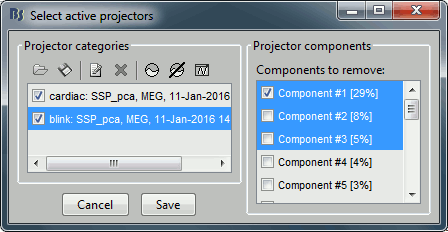
Select the first three components and display their topographies:
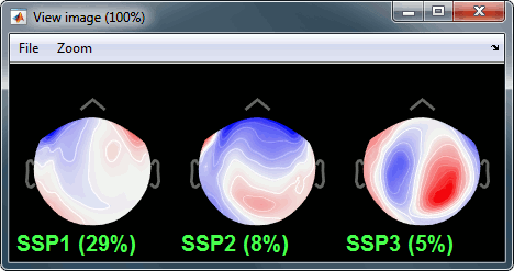
Component #1: Most likely a blink,
Component #2: Probably a saccade (another type of eye movement),
- Component #3: Not related with the eye movements (maybe related with the alpha activity).
As a side note, if you had not selected the option "Compute using existing SSP/ICA projectors", you would have obtained the projectors below, which correspond to the topography of the artifact in the original signals (without considering the cardiac projector). It is normal if the topographies we obtain after removing the cardiac peaks are slightly different, this is because they are computed on the different subspace of the signals. The relative singular values is smaller after the cardiac correction, maybe because the recordings we used to compute it already contained some eye movements.
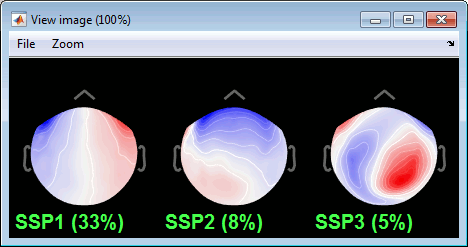
Display the times series for these three components, together with the EOG signals. You have to uncheck temporarily the component #1 to be able to display its signal. When it is checked, it is removed from the signal therefore it corresponds to a flat trace.
The figure below shows the EOG and SSP values between 318s and 324s. The SSP1 trace matches the blink observed in VEOG and SSP2 matches the saccade observed in HEOG.
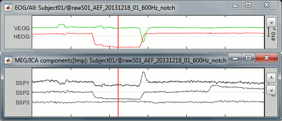
Left-temporal MEG signals when there is no component selected:
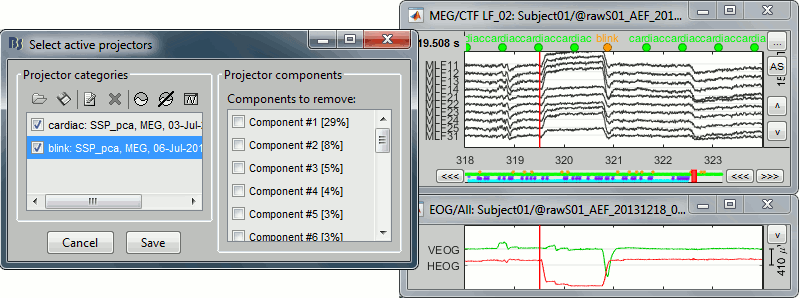
With only the component #2 selected (saccade):
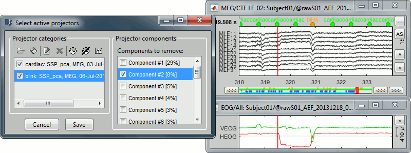
With components #1 and #2 selected (blink + saccade):

Keep the components #1 and #2 selected and click on [Save] to validate your changes.
Run #02
Reproduce the same operations on Run #02:
- Close everything with the [X] button at the top-right corner of the Brainstorm window.
Open the MEG recordings for run AEF #02 (double-click on the file link).
Artifacts > SSP: Heartbeats: Event name "cardiac", sensors "MEG", use existing SSP projectors.
Select component #1, click on [Save].
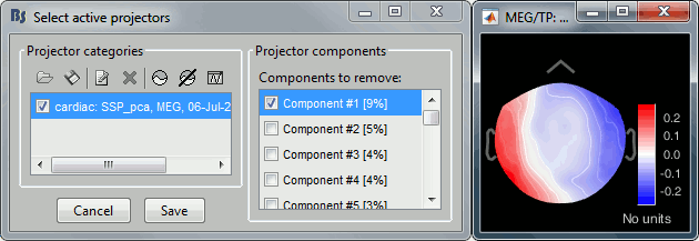
Artifacts > SSP: Eye blinks: Event name "blink", sensors "MEG", use existing SSP projectors.
Select component #1, click on [Save].
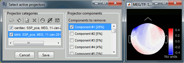
- Note that in this second session, the representation of the saccade was not as clear as in the first file. The distribution of the percentage values does not show any clear component other from the blink one, and the topographies are not as clear. In general, the saccade processing requires a separate step, we will illustrate this in the next tutorial.
Note for beginners
Everything below is advanced documentation, you can skip it for now.
SSP: Generic
The calculation of the SSP for the heartbeats and the eye blinks are shortcuts to a more generic process "Artifacts > SSP: Generic". You may need this process if the standard parameters do not work of if you want to use this technique to remove other types of artifacts.
Time window: What segment of the file you want to consider.
Event name: Markers that are used to characterize the artifact. If you don't specify any event name, it will use the entire time window as the input of the PCA decomposition.
Event window: Time segment to consider before and after each event marker. We want this time window to be longer than the artifact effect itself, in order to have a large number of time samples representative of a normal brain activity. This helps the PCA decomposition to separate the artifact from the ongoing brain activity.
Frequency band: Definition of the band-pass filter that is applied to the recordings before calculating the projector. Usually you would use the same frequency band as we used for the detection, but you may want to try to refine this parameter if the results are not satisfying.
Sensor types or names: List of sensor names or types for which the SSP projectors are calculated. You can get better results if you process one sensor type at a time.
Compute using existing SSP/ICA projectors: Same as in the heartbeats/blinks processes.
Save averaged artifact in the database: If you check this option with an event name selected, the process will save the average of all the artifact epochs (event marker + event window) before and after the application of the first component of the SSP decomposition. This is illustrated in the next section.
Method to calculate the projector:
PCA: What was described until now: SVD decomposition to extract spatial components.
Average: Uses only one spatial component, the average of the time samples at which the selected events occur. This has no effect if there are no events selected.
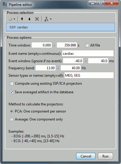
Averaged artifact
One efficient way of representing the impact of this artifact correction is to epoch the recordings around the artifacts before and after the correction and compute the average of these epochs.
- Run the process "SSP: Generic" with:
- The default blink options: event "blink", [-200,+200]ms, [1.5-15]Hz.
The option "Computing existing SSP/ICA projectors" disabled.
The option "Save averaged artifact in the database" selected.
- The option panel should look like the screen capture in the previous section.
Look at the topography of the first component. You can notice that the percentage value is higher than what we got previously, and that the topography looks different than previously.
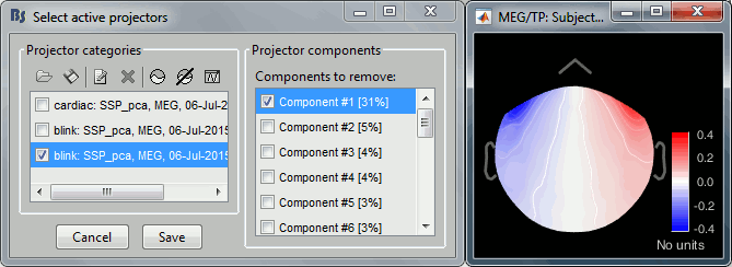
- This difference comes from the fact that this time we did not use the cardiac SSP to compute the blink SSP ("Compute existing SSP" disabled). This could indicate that there is some form of cross-contamination of the "blink" and "cardiac" events that we designed here. The origin of the common signals between the different segments of artifact is sometimes due to important alpha waves (around 10Hz) that are present for most of the recordings. It don't matter much, you just have to remember that the computation order matters and that you can try variations of the suggested workflow to fit better your recordings.
- Otherwise, the difference between this topography and the previous one could be only due to the fact that they represent the artifact in different subspaces (in the first case, one dimension has already been removed). Even if the two artifacts were completely independant (the two removed dimensions are orthogonal), the topographies would look slightly different.
You should see now two additional files in your database. They are both the average of the 19 blinks identified in the recordings, [-200,+200]ms around the "blink" events. The top row shows the average before the SSP correction, the bottom row the same average but recomputed after removing the first component of the decomposition. The artifact is gone.
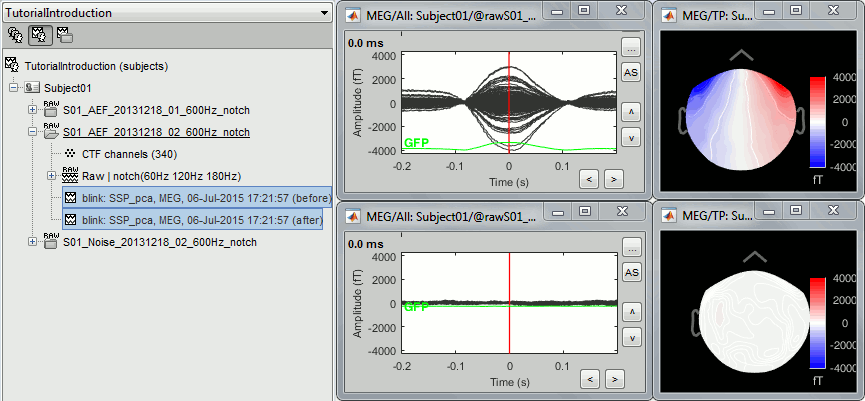
Delete this new category, and make sure you get back to the previous settings (first component of both "cardiac" and "blink" selected). Click on [Save] to validate this modification.
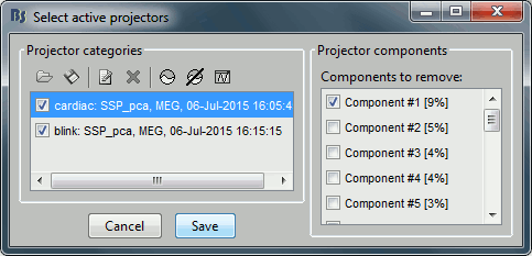
Troubleshooting
You have calculated your SSP projectors as indicated here but you don't get any good results. No matter what you do, the topographies don't look like the targeted artifact. You can try the following:
- Review one by one the events indicating the artifacts, remove the ones that are less clear or that occur close to another artifact.
- Select or unselect the option "Compute using existing SSP".
- Change the order in which you compute the projectors.
- Use the process "SSP: Generic" and modify some parameters:
- Use a narrower frequency band: especially the EOG, if the projectors capture some of the alpha oscillations, you can limit the frequency band to [1.5 - 9] Hz.
- Reduce or increase the time window around the peak of the artifact.
- Change the method: Average / SSP.
- If you have multiple acquisition runs, you may try to use all the artifacts from all the runs rather than processing the files one by one. For that, use the Process2 tab instead of Process1. Put the "Link to raw file" of all the runs on both sides, Files A (what is used to compute the SSP) and Files B (where the SSP are applied).
Always look at what this procedure gives you in output. Most of the time, the artifact cleaning will be an iterative process where you will need several experiments to adjust the options and the order of the different steps in order to get optimal results.
SSP Theory
The Signal-Space Projection (SSP) is one approach to rejection of external disturbances. Here is a short description of the method by Matti Hämäläinen, from the MNE 2.7 reference manual, section 4.16.
Unlike many other noise-cancellation approaches, SSP does not require additional reference sensors to record the disturbance fields. Instead, SSP relies on the fact that the magnetic field distributions generated by the sources in the brain have spatial distributions sufficiently different from these generated by external noise sources. Furthermore, it is implicitly assumed that the linear space spanned by the significant external noise patterns has a low dimension.
Without loss of generality we can always decompose any n-channel measurement b(t) into its signal and noise components as:
b(t) = bs(t) + bn(t)
Further, if we know that bn(t) is well characterized by a few field patterns b1...bm, we can express the disturbance as
bn(t) = Ucn(t) + e(t) ,
where the columns of U constitute an orthonormal basis for b1...bm, cn(t) is an m-component column vector, and the error term e(t) is small and does not exhibit any consistent spatial distributions over time, i.e., Ce = E{eeT} = I. Subsequently, we will call the column space of U the noise subspace. The basic idea of SSP is that we can actually find a small basis set b1...bm such that the conditions described above are satisfied. We can now construct the orthogonal complement operator
P⊥ = I - UUT
and apply it to b(t) yielding
b(t) ≈ P⊥bs(t) ,
since P⊥bn(t) = P⊥Ucn(t) ≈ 0. The projection operator P⊥ is called the signal-space projection operator and generally provides considerable rejection of noise, suppressing external disturbances by a factor of 10 or more. The effectiveness of SSP depends on two factors:
The basis set b1...bm should be able to characterize the disturbance field patterns completely and
The angles between the noise subspace space spanned by b1...bm and the signal vectors bs(t) should be as close to π/2 as possible.
If the first requirement is not satisfied, some noise will leak through because P⊥bn(t) ≠ 0. If the any of the brain signal vectors bs(t) is close to the noise subspace not only the noise but also the signal will be attenuated by the application of P⊥ and, consequently, there might by little gain in signal-to-noise ratio.
Since the signal-space projection modifies the signal vectors originating in the brain, it is necessary to apply the projection to the forward solution in the course of inverse computations.
SSP Algorithm
The logic of the SSP computation is the following:
- Take a small time window around each marker to capture the full effect of the artifact, plus some clean brain signals before and after. The default time window is [-200,+200]ms for eye blinks, and [-40,+40]ms for the heartbeats.
- Filter the signals in a frequency band of interest, in which the artifact is the most visible (in practice, we extract a segment long enough so that it can be filtered properly, and cut it after filtering).
Concatenate all these time blocks into a big matrix A = [b1, ..., bm]
Compute the singular value decomposition of this matrix A: [U,S,V] = svd(A, 'econ')
The singular vectors Ui with the highest singular values Si are an orthonormal basis of the artifact subspace that we want to subtract from the recordings. The software selects by default the vector with the highest eigenvalue. Then it is possible to redefine interactively the selected components.
Calculate the projection operator: P⊥i = I - UiUiT
Apply this projection on the MEG or EEG recordings F: F = P⊥iF
The process has to be repeated separately several times for each sensor type and each artifact.
Steps #1 to #5 are done by the processes "Artifact > SSP" in the Record tab: the results, the vectors Ui, are saved in the channel file (field ChannelMat.Projector(i).Components).
Steps #6 and #7 are calculated on the fly when reading a block of recordings from the continuous file: when using the raw viewer, running a process a process on the continuous file, or importing epochs in the database.
Step #8 is the manual control of the process. Take some time to understand what you are trying to remove and how to do it. Never trust blindly any fully automated artifact cleaning algorithm, always check manually what is removed from the recordings, and do not give up if the first results are not satisfying.
Extract the time series
It could be useful to save the SSP or ICA time series in a new file for further processing. Here is one solution to get there:
First, make sure you do not remove the components you are interested in: open the continuous recordings, Record tab > Artifacts > Select active projectors, unselect the components you want to study, so that they are kept in the imported data.
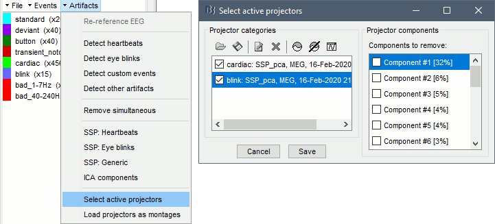
Import the segments of recordings of interest from the continuous file: select the option Apply SSP/ICA projectors, otherwise the projectors would be discarded from the new channel file in the imported folder.
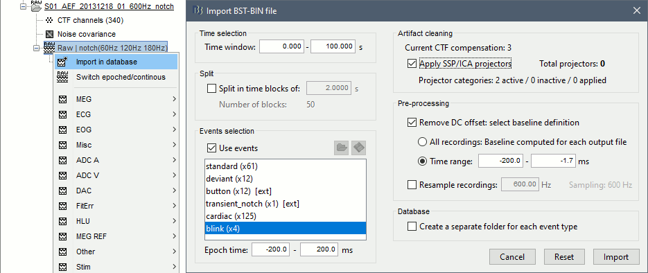
To review the SSP/ICA time series (optional): open the recordings you just imported, and select the menu Artifacts > Load projector as montages in the Record tab. The projectors are made available in the montage menu.
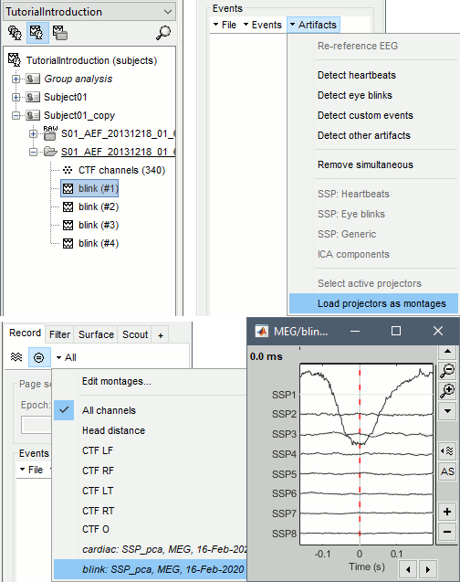
To create a new file with the SSP/ICA time series in the database: select the file you imported in Process1 and run the process Standardize > Apply montage, with the option Create new folders selected.

On the hard drive
The projectors are saved in the channel file associated with the recordings. This means that they will be shared by all the files that share the same channel file. As a consequence, you cannot share the channel files between acquisition runs if you are planning to use different SSP projectors for different runs.
You can find them in the field ChannelMat.Projector (array of structures):
Comment: String representing the projector in the window "Select active projectors".
Components: [Nsensors x Ncomponents], each column is one spatial component.
CompMask: [1 x Ncomponents], Indicates if each component is selected or not (0 or 1).
Status: 0=Category not selected, 1=Category selected, 2=Projectors already applied to the file.
SingVal: [1 x Ncomponents], Singular values of the SVD decomposition for each component.
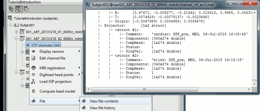
Additional documentation
Articles
- C. D. Tesche, M. A. Uusitalo, R. J. Ilmoniemi, M. Huotilainen, M. Kajola, and O. Salonen, "Signal-space projections of MEG data characterize both distributed and well-localized neuronal sources," Electroencephalogr Clin Neurophysiol, vol. 95, pp. 189-200, 1995.
- M. A. Uusitalo and R. J. Ilmoniemi, "Signal-space projection method for separating MEG or EEG into components," Med Biol Eng Comput, vol. 35, pp. 135-40, 1997.
Tutorials and forum discussions
Tutorial: SSP cookbook
Additional SSP examples can be found in the tutorials in section Other analysis scenarios.
Tutorial 14: Additional bad segments
Authors: Francois Tadel, Elizabeth Bock, Sylvain Baillet
We have already corrected the recordings for the artifacts at fixed frequencies (power lines) and for some standard and reproducible artifacts (heartbeats and blinks). There are many other possible sources of noise that can make the recordings unusable in our analysis. This tutorial introduces how to identify and mark these bad segments.
Contents
Manual inspection
It is very important to mark bad segments (noisy sections) of the recordings before running any fancy analysis. It may save you hours of repeated work later, when you discover after processing all your data that you have to redo everything because you have left some huge artifacts in the recordings.
In terms of quality control, there is no automatic method that will give you results as good as a manual screening of the recordings. We recommend you always take a few minutes to scroll through all your files to identify and tag all the noisy segments. Do this full screening after you're done with all the other pre-processing steps (filtering and SSP/ICA cleaning) to remove what has not been corrected with other techniques.
At the beginning, it is not easy to separate what is too noisy from what is acceptable. This is usually an iterative process: at the first attempt you guess, you average the trials and estimate the sources and finally realize that are some eye movements left that are masking your effect of interest. You have to delete everything, add some bad segments and try again. On the contrary, if you reject too much data at the beginning, you may not have enough trials to observe your effect correctly. The balance is not easy to find, but you'll get good at it quickly. Brainstorm offers tools to do these operations easily, so a few trials and errors are not too dramatic. Just make sure you check the quality of your data at every step of the analysis, so that you don't go too far in the wrong direction.
To review your recordings and check for major artifacts, you can for instance:
- Display all the sensors in columns, you don't need to see each sensor individually.
- Use a large time window (page duration = 5-20s).
- Increase the gain of the sensors to see clearly the abnormally large values.
Scroll using the shortcuts corresponding to buttons [<<<] and [>>>]: F3, Shift+F3, F4, etc.
- Unselect the autoscale option ([AS] button on the right side of the figure) so that the amplitude doesn't change every time you move to the next page, it will make the review easier.
When you identify something that doesn't look good:
- Click and move your mouse to select the segment you consider as noisy.
Mark the segment as bad: Right-click > Reject time segment (or Ctrl+B).
The example below shows Run #02 from 206s to 211s:
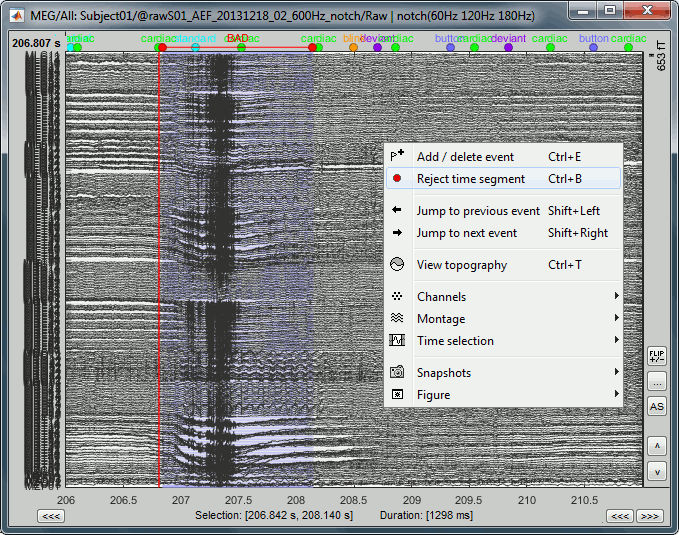
Automatic detection
We have developed some tools to help with this screening procedure. The process "Artifacts > Detect other artifacts" identifies epochs of time that contain typical artifacts from eye movement, subject movement or muscle contractions. While it is still advised that you visually inspect all of your data, this process can help identify areas that contain artifacts which you may want to mark as bad segments.
Currently, the process runs only on continuous raw links and identifies artifacts in two frequency bands, chosen because of the predictability of artifacts in these bands.
1-7 Hz: Typically related to subject movement, eye movements and dental work (or other metal)
40-240 Hz: Related to muscle noise and some sensor artifacts
- Note that the alpha band (8-12 Hz) is specifically avoided here since some alpha oscillations can be quite high in amplitude and falsely detected as artifact.
Important notes
- Before running this detection it is highly recommended that you run the cleaning processes for cardiac and eye blink artifacts.
This process is currently being tested. If you find a bug or have other comments related to its performance, please provide comments here or on the user forum.
- We recommend you use the markers that this process creates as suggestions, not as the actual reality. Do not use this method fully automatically, always review its results.
Recommendations for usage
- Start by running the process on one run per subject. Scan though the recording and confirm that the detection is performing well.
- Adjust the threshold as needed, then run the detection on the other runs for that subject.
If there are many eye movements, the "1-7 Hz" detection can work well for computing an SSP projector. This is done using the menu "Artifacts > SSP: Generic" as described below. If a suitable projector is found and applied, re-run the artifact detection to find the remaining artifacts that were not removed.
Run #01
We will now apply this process on the first acquisition session:
Double-click on the link to show the MEG sensors for Run #01.
The process will exclude the segments that are already marked as bad from the detection. If you have marked bad segments at the beginning of this tutorial, delete them all: Select the category "BAD" and press the delete key, or menu Events > Delete group.
In the Record tab, select the menu: "Artifacts > Detect other artifacts".
Time window: The time window for which the detection will be performed.
Sensitivity: 1 is very sensitive, 5 very conservative, 3 works well for a variety of conditions.
Frequency band selection: Check the box for which band(s) you will perform the detection.
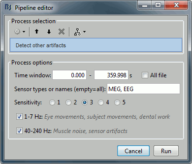
After running the process, event types are created, one for each frequency band. They contain extended events indicating the start and end of the epoch. The time resolution is 1 second and therefore the epoch may, in fact, be a bit longer than the actual artifact. You can manually refine the time definition if you wish and mark some or all events as bad.

- Check quickly the segments that were marked as possible artifacts. They all correspond to some form of irregularities in the recordings but there are very few of them. We will just flag all the segments detected in both categories as bad.
For considering these events as bad, select them both in the events list and use the menu
"Events > Mark group as bad". Alternatively, you can rename the events and add the tag "bad_" in their name, it would have the same effect.
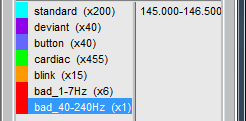
- Unload all the data with the [X] in the toolbar of the Brainstorm window. Save the modifications.
Run #02
Repeat the same operation on the second data file:
Double-click on the link to show the MEG sensors for Run #02.
Run the menu "Artifacts > Detect other artifacts" with the same parameters as the first file.

- The category "1-7Hz" contains many saccades, maybe enough for computing an SSP projector.
If you are not interested in seeing how to remove the saccades with SSP projectors, just mark the two groups as bad: with the menu "Events > Mark group as bad", or renaming them in "bad_1-7Hz" and "bad_40-240Hz". Then go directly to the next tutorial.
Saccade SSP
This run #02 is a good example to illustrate how we can use SSP projectors to remove the artifacts caused by eye saccades. You could mark the saccades manually or use the pre-selection available in "1-7Hz".
Rename category "1-7Hz" in "saccade" and delete category "40-240Hz".
Open the EOG recordings at the same time: right-click on file > EOG > Display time series.
Keep only the saccades: Delete all the events that do not show a clear step in the HEOG channel.
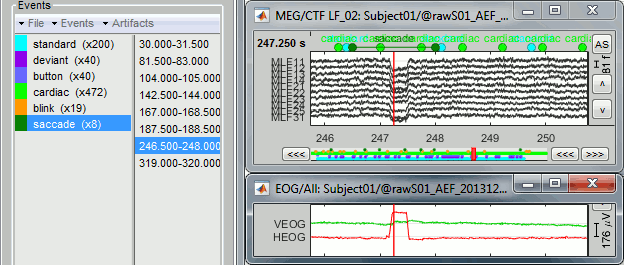
Run the process "Artifacts > SSP: Generic" with the following options:
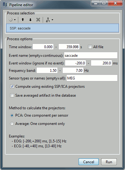
Note: the event window option will not be used because the events "saccade" are extended events and already include their duration.
The first component removes the artifact very well. Keep it selected and click on [Save].
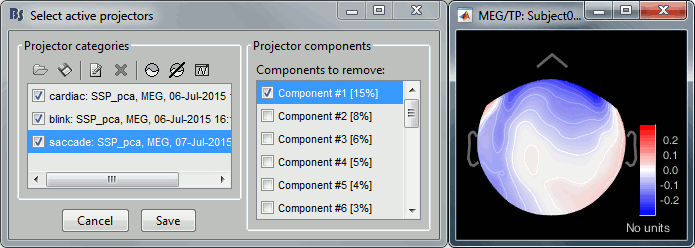
Run again the process "Detect other artifacts". There are now less events detected in 1-7Hz.
Rename the categories in "bad_1-7Hz" and "bad_40-240Hz" to flag them as bad segments.
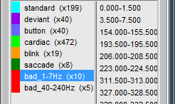
Elekta-Neuromag SQUID jumps
MEG signals recorded with Elekta-Neuromag systems frequently contain SQUID jumps. They are easy to spot visually in the recordings, they look like sharp steps followed by a change of baseline value. These jumps are due to the instability of the electronics, which fails at controlling the state of the SQUID during the recording sessions.
These steps cause important issues in the analysis of the signal, both in amplitude and in frequency. They are difficult to detect and remove, especially when some pre-processing with the Elekta software has already been applied. Running MaxFilter/SSS on MEG recordings with a SQUID jump on one sensor propagates the artifact to all the sensors.
The best approach is to remove these jumps from the analysis:
By marking them as bad segments manually, if their number is reasonable (in Brainstorm).
The 1-7Hz artifact detection employed here will usually catch them.By marking the sensors as bad if only a few of them are affected (before running MaxFilter).
By computing SSP projectors to remove the jumps (before running MaxFilter/SSS).
As of today, this approach is possible only if you use MNE or MNE-Python for the early stages of pre-processing. When the free SSS algorithm implemented in MNE-Python is made available in Brainstorm, we will be able to use this approach in Brainstorm as well.
An example before MaxFilter (SQUID jump visible on one sensor only):
Examples after MaxFilter (SQUID jump propagated on all the sensors):
Additional documentation
Tutorial: SSP cookbook
Tutorial 15: Import epochs
Authors: Francois Tadel, Elizabeth Bock, Sylvain Baillet
We can consider that our datasets are clean from any major artifact. We will now proceed to the analysis of the brain signals we recorded in response to the auditory stimulation. There are two major types of processing workflows for MEG/EEG, depending on whether we are dealing with an event-related paradigm or a steady-state/resting-state study.
This tutorial will only focus on the event-related case: series of stimuli are sent to the subject and we have the corresponding triggers marked in the recordings. We will base our analysis on these triggers, import short epochs around each of them and average them. You will find in the advanced tutorials a scenario of MEG resting-state analysis.
Contents
Import in database
Until now, we've only been looking at data that was read from continuous files. The raw file viewer provides rapid access to the recordings, but many operations can only be applied to short segments of recordings that have been imported in the database. We will refer to these as "epochs" or "trials".
Right-click on Run#01 > Import in database.
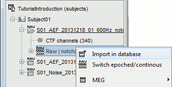
Set the import options as described below:
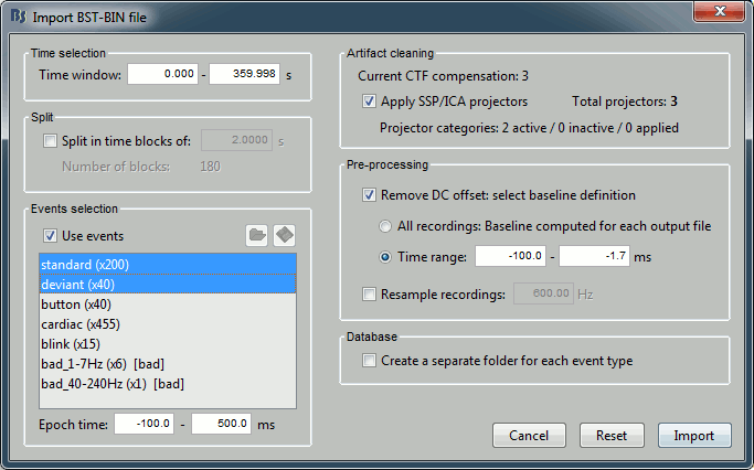
Time window: Time range of interest. We are interested by all the stimulations, so do not change this parameter. The default values always represent the entire file.
Split: Useful to import continuous recordings without events, to import successive chunks of the same duration. We do not need this here.
Events selection: Check the "Use events" option, and select both "standard" and "deviant".
The number between parenthesis represents the number of occurrences of each event in the selected time window (changes if you modify the time definition at the top of the window)Epoch time: Time segment that is extracted around each event marker. Set it to [-100,+500]ms.
This option is disabled for extended events: if you want to enable it, you need to convert the extended events to simple events first.Apply SSP/ICA projectors: Use the active projectors calculated during the previous pre-processing steps. Always check the summary of the projectors that are selected.
Here there are 2 categories ("cardiac" and "blink") with a total of 3 projectors selected (one in "cardiac" and two in "blink", the blink and the saccade). Keep this option selected.Remove DC Offset: Check this option, select Time range: [-100, -1.7]ms. For each epoch, it will:
- Compute the average of each channel over the baseline (pre-stimulus interval: [-100,-1.7]ms)
- Subtract it from the channel at every time instant (full epoch interval: [-100,+500]ms).
- This option removes the baseline value of each sensor. In MEG, the sensors record variations around a somewhat arbitrary level, therefore this operation is always needed, unless it was already applied during one of the pre-processing steps.
Resample recordings: Keep this unchecked.
Create a separate folder for each epoch type: Do not check this option.
- If selected: a new folder is created for each event type ("standard" and "deviant")
- If not selected: all the epochs are saved in a new folder, the same one for all the events, that has the same name as the initial raw file. This is what we want because we have two acquisition runs with different channel files (different head positions and different SSP projectors) to import for the same subject. If we select this option, the "standard" epochs of both runs would be imported in the same folder and would end up sharing the same channel file, which is not correct.
One new folder appears in Subject01. It contains a channel file and two trial groups.
- The channel file is copied from the continuous file.
- To expand a group of trials and show all the files: double-click on it or click on the "+" next to it.
- The SSP projectors calculated in the previous tutorial were applied on the fly while reading from the continuous file. These epochs are clean from eye blinks and power line contamination.
Note that the trials that are overlapping with a BAD segment are tagged as bad in the database explorer (marked with a red dot). All the bad trials are going to be ignored in the rest of the analysis, because they are ignored by the Process1 and Process2 tabs (see next tutorial).
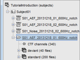
Review the individual trials
After reviewing the continuous file with the "columns" view (channels one below the other) it can be useful to also review the imported trials with the "butterfly" view (all the channels superimposed).
- Double-click on the first trial for the "deviant" condition.
Switch to the "butterfly" display mode: in the Record tab, click on the first button in the toolbar.
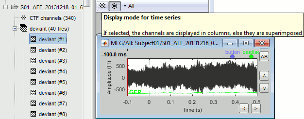
Right-click on the figure > Navigator > Next data file, or use the keyboard shortcut F3.
This way you can quickly review all the trials to make sure that there is no obvious problem.
Mac users: The keys "Fx" are obtained by holding the "Fn" key simultaneously.
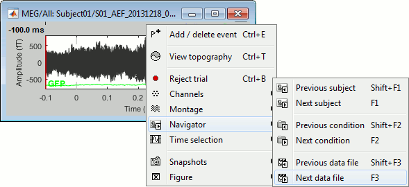
To manually tag a trial as bad, you have three options:
Right-click on the trial file in the database > Reject trial.
Right-click on the figure > Reject trial.
Use the keyboard shortcut Ctrl+B.
To set all the trials back as good in a group: right-click on the trials group > Accept bad trials.
Raster plot
You can also get an overview of the values of one specific sensor over all the trials at once.
Right-click on the group of trials "deviant" > Display as image > MEG.
- You can change the selected sensor with drop-down menu in the Display tab, or use the up/down arrows on your keyboard after clicking on the figure.
The bad trials are already marked, but if they were not this view could help you identify them easily.
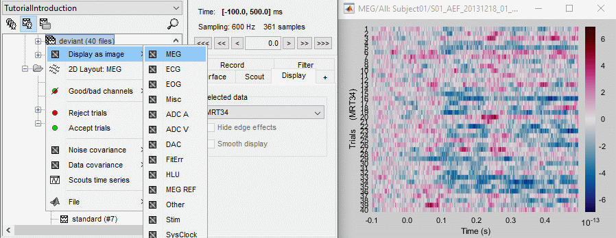
Run #02
Repeat the same operations for the second dataset:
Right-click on Run#02 > Import in database.
Import events "standard" and "deviant" with the same options.
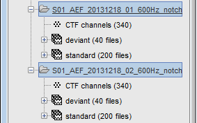
Epoch length
We imported epochs of 600ms (100ms baseline + 500ms post-stimulus) but did not justify this choice.
The length of the epochs you import should be chosen very carefully. If you realize later your epochs are too short or too long, you would have to start over your analysis from this point.
The epoch length to consider depends on:
The experimental design
- The minimum duration between two stimuli defines the maximum length you can consider analyzing after the stimulus. You should design your experiment so that it always includes the entire evoked response, plus an additional segment that you can use as a baseline for the following epoch.
- In this study, the inter-stimulus interval (ISI) is random between 0.7s and 1.7s. The minimum ISI (700ms) is long enough to include the entire auditory evoked response, but not the button press that follows a deviant tone. In some cases (late subject response and short ISI), the following stimulation occurs while the brain is still processing the button press. The baseline of some epochs may contain motor and somatosensory components.
- For data processing, it is always better to have longer ISI, but it also means increasing the duration of the experiment or decreasing the number of repetitions, which leads to other problems. The trade-off between data quality and recording time in this experiment is acceptable, very few trials are actually contaminated by the motor response to the previous trial. We will ignore this problem in the following tutorials, but you could decide to reject these few trials in your own analysis.
Here we consider only a short baseline (100ms) to avoid including too much motor activity.
We will only study the auditory response, therefore 500ms post-stimulus is enough.
The processing pipeline
You may have to artificially extend the epochs of interest for technical reasons. Most filters cause edge effects, ie. unreliable segments of data at the beginning and the end of the signal. When applied on short epochs, they might destroy all the data of interest.
For avoiding this, you can add a few hundred milliseconds before and after your epoch of interest. It doesn't matter if it overlaps with the previous or the next epoch. After running the operations that required longer signals, you can cut your epochs back to the desired epoch length. Examples:
Time-frequency (Morlet wavelets):
When estimating the power at frequency f Hz, you get incorrect values for at least one period (T=1/f) at the beginning and the end of the signal. For example, at 2Hz you need to discard the first and last 500ms of your time-frequency maps (1/2Hz=0.5s).Low-pass filtering:
With any filtering operation there will always be a transient effect at the beginning of the filtered data. After filtering, you need to discard the time windows corresponding to these effects. Their duration depends on the order of the filter: this is documented in the tutorial Power spectrum and frequency filters.Hilbert transform:
Same considerations as for the low-pass filter. This process starts by filtering the signals in various frequency bands, using the same function as the band-pass and low-pass filters.Normalizations:
The normalization procedures that use a baseline from the same epoch (Z-score, ERS/ERD, baseline correction) usually work better with longer baselines. The longer the clean baseline, the better the estimation of the average and standard deviation over this baseline. If your baseline is too short, the quality of your normalization will be low.
If you normalize time-frequency maps or filtered source averages, you have to additionally exclude the edge effects from the baseline, and consider an even longer baseline.
In this tutorial, we decided to work with very short epochs (600ms only) so that all the analysis would run on most computers, including personal laptops. For any type of frequency analysis on the recordings, this will be too short. When processing your own recordings, you should increase the size of the epochs beyond the segment that you are actually planning to study.
On the hard drive
Right-click on any imported epoch > File > View file contents:
Structure of the imported epochs: data_*.mat
F: [Nchannels x Ntime] recordings time series, in Volts.
Std: [Nchannels x Ntime] Standard deviation or standard error, when available (see next tutorial).
Comment: String displayed in the database explorer to represent this file.
ChannelFlag: [Nchannels x 1] One value per channel, 1 means good, -1 means bad.
Time: [1 x Ntime] Time values for each sample recorded in F, in seconds.
DataType: Type of information saved in the F matrix.
Device: Name of the acquisition system used to record this file.
Leff: Effective number of averages. For averaged files, number of trials that were used to compute this file.
Events: Time markers available in the file (stimulus triggers or other events)
label: Name of the event group.
color: [r,g,b] Color used to represent the event group, in Matlab format.
epochs: [1 x Nevt] Only ones for imported epochs.
times: [1 x Nevt] Time in seconds of each marker in this group (times = samples / sfreq).
For extended events: [2 x Nevt], first row = start, second row = end.reactTimes: Not used anymore.
select: Indicates if the event group should be displayed in the viewer.
channels: {1 x Nevt} Cell array of cell-arrays of strings. Each event occurrence can be associated with one or more channels, by setting .channels{iEvt} to a cell-array of channel names.
notes: {1 x Nevt} Cell-array of strings: additional comments for each event occurrence
hedTags: {1 x NhedTags} Cell-array of strings: HED tags for this event group.
T0: Timestamp with milliseconds to indicate the time 0s in the recording.
History: Operations performed on file since it was imported (menu "View file history").
File history
Right-click on any imported epoch > File > View file history:
List of bad trials
There is no field in the file structure that says if the trial is good or bad.
This information is saved at the level of the folder, in the brainstormstudy.mat file.Right-click on an imported folder > File > Show in file explorer.
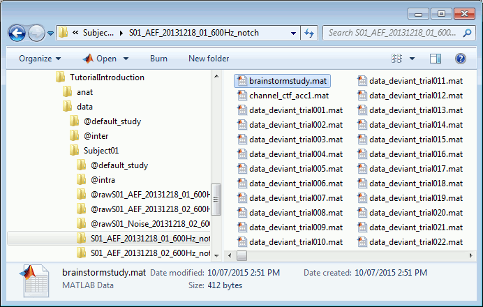
Load the brainstormstudy.mat file into Matlab, the bad trials are listed in the cell array "BadTrials":
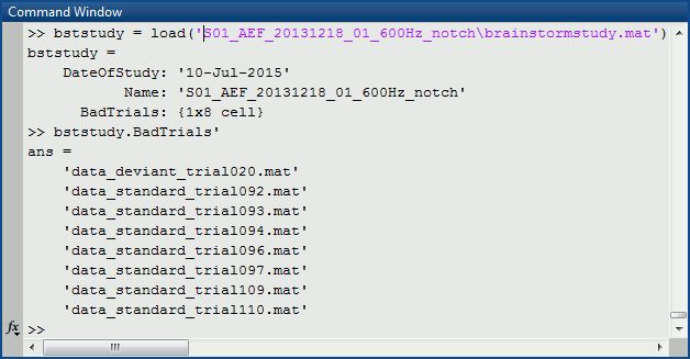
Useful functions
in_bst_data(DataFile, FieldsList): Read an imported epoch.
in_bst(FileName, TimeWindow): Read any Brainstorm data file with the possibility to load only a specific part of the file. "TimeWindow" is a range of time values in seconds: [tStart, tStop].
bst_process('LoadInputFile', FileName, Target, TimeWindow): The most high-level function for reading data files. "Target" is a string with the list of sensor names or types to load.
Additional documentation
Forum: Different epoch length
Tutorial 16: Average response
Authors: Francois Tadel, Elizabeth Bock, Sylvain Baillet
All the epochs we have imported in the previous tutorial are represented by matrices that have the same size (same number of channels, same number of time points), therefore they can be averaged together by experimental condition. The result is called indifferently "evoked response", "average response", "event-related field" in MEG (ERF) or "event-related potential" in EEG (ERP). It shows the components of the brain signals that are strictly time-locked to the presentation of a stimulus.
Contents
Averaging
We will now compute the average responses for both the "standard" and "deviant" conditions. Two constraints have to be taken into consideration at this stage.
Averaging runs separately: With MEG, it is not recommended to average sensor data across acquisition runs with different head positions (ie. different "channel files"). If the head of the subject moved between two blocks of recordings, the sensors do not record the same parts of the brain before and after, therefore the runs cannot be compared directly. With EEG, you can generally skip this recommendation.
Number of trials: When computing subject-level averages for experimental conditions with different number of trials, you have two options. You can either use the same number of trials for all the conditions and subjects (to make them "more comparable") or use all the available good trials (more samples lead to better estimations of the mean and variance). Here we will go with the second option, using all the trials. See this advanced section for more details.
Drag and drop all the "standard" and "deviant" trials for both runs in Process1.
In the Process1 box, the number of imported trials (comment in the database explorer, eg. "40 files") does not match the number of files selected for processing (between brackets, eg. "[39]"). This difference is due to the bad trials that we have in these folders. The trials tagged with a red dot in the database explorer are ignored by all the processes. The total number of selected files is 457 instead of 479, it means that we have a total of 22 bad trials.
Select the process "Average > Average files".
Select the options: By trial group (folder), Arithmetic average, Keep all the event markers.
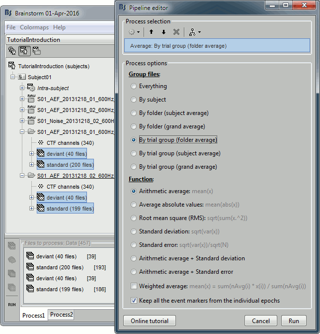
You get two new files for each acquisition run. The number between parenthesis indicates how many good trials were used to compute each average.
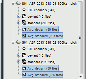
Process options: Average
Description of all the options of the process: Average > Average files.
Everything: Averages all the files selected in Process1 together, creates only one file in output.
By subject: Groups the files by subject (ignoring the folders), creates one file per subject.
By folder (subject average): Groups by subject and by folder, ignoring the trial groups.
In the current configuration, it would produce two files, one for each acquisition run.By folder (grand average): Groups by folder, across the subjects. All the files located in folders with the same name would be averaged together, no matter in what subject they are.
By trial group (folder average): Groups by set of trials with the same name, separately for each folder and each subject. Here it creates four groups (two folders x two trial groups).
By trial group (subject average): Groups by set of trials with the same name, for each subject. The separation in folders is ignored. Here it would produce two files (deviant and standard).
By trial group (grand average): Groups by set of trials with the same name, ignoring the classification by folder or subject.
Function: Documented directly in the option panel.
Weighted average: When averaging single trials, the number of files is saved in the field Leff of the average file. When re-averaging the averages across acquisition sessions or subjects, this field Leff can be used to weigh each file with the number of trials from which it was computed:
mean(x) = sum(Leff(i) * x(i)) / sum(Leff(i))
In most cases, this option should be selected when averaging within a subject and disabled when averaging across subjects. It has no impact in the current example (no averages, Leff=1).Keep all the event markers: If this option is selected, all the event markers that were available in all the individual trials are reported to the average file. It can be useful to check the relative position of the artifacts or the subject responses, or quickly detect some unwanted configuration such as a subject who would constantly blink immediately after a visual stimulus.
Visual exploration
The average response contains interesting information about the brain operations that occur shortly after the presentation of the stimulus. We can explore two dimensions: the location of the various brain regions involved in the sensory processing and the precise timing of their activation. Because these two types of information are of equal interest, we typically explore the recordings with two figures at the same time, one that shows all the signals in time and one that shows their spatial distribution at one instant.
Open the MEG recordings for the deviant average in Run#01: double-click on the file.
- In the Record tab: Select the "butterfly" view more (first button in the toolbar).
In the Filter tab: Add a low-pass filter at 40Hz.
In the Record tab: Delete the "cardiac" event type, we are not interested by their distribution.

This figure shows a typical clean evoked response, with a high signal-to-noise ratio. This represents the brain response to a simple auditory stimulation, the large peak around 90ms probably corresponds to the main response in the primary auditory cortex.
The green line represents the global field power (GFP), i.e. the standard deviation of all the sensors values at each time point. This measure is sometimes used to identify transient or stable states in ERP/ERF. You can hide it with the display options menu Extra > Show GFP.
- This is the response to the deviant beeps (clearly higher in pitch), for which the subject is supposed to press a button to indicate that he/she detected the target. These responses are represented with the "button" events, distributed between 350ms and the end of the file (many responses happened after 500ms). Because of the variability in the response times, we can already anticipate that we won't be able to study correctly the motor response from this average. For studying the activity in the motor area, we need to epoch the recordings again around the "button" events.
Add a spatial view:
Open a 2D topography for the same file (right-click on the figure > View topography, or Ctrl+T).
Review the average as a movie with the keyboard shortcuts (hold the left or right arrow key).
At 90ms, we can observe a typical topography for a bilateral auditory response. Both on the left sensors and the right sensors we observe field patterns which seem to indicate a dipolar-like activity in the temporal or central regions.
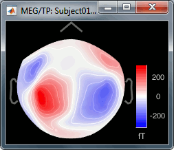
Close everything with the button [X] in the top-right corner of the Brainstorm window.
Accept to save the modifications (you deleted the "cardiac" events).- Open the "standard" average in the same way and delete the "cardiac" markers.
Repeat the same operations for Run#02:
- Open the MEG recordings for deviant and standard.
- Delete the "cardiac" markers in both files.
- Open a 2D topography and review the recordings.
- Close everything.
Interpretation
Let's display the two conditions "standard" and "deviant" side-by-side, for Run#01.
Right-click on average > MEG > Display time series.
Right-click on average > MISC > Display time series (EEG electrodes Cz and Pz)
Right-click on average > MEG > 2D Sensor cap
In the Filter tab: add a low-pass filter at 40Hz (it makes the figures easier to read).
In the Record tab: you can set a common amplitude scale for all the figures with the button [=].
Here are the results for the standard (top) and deviant (bottom) beeps:
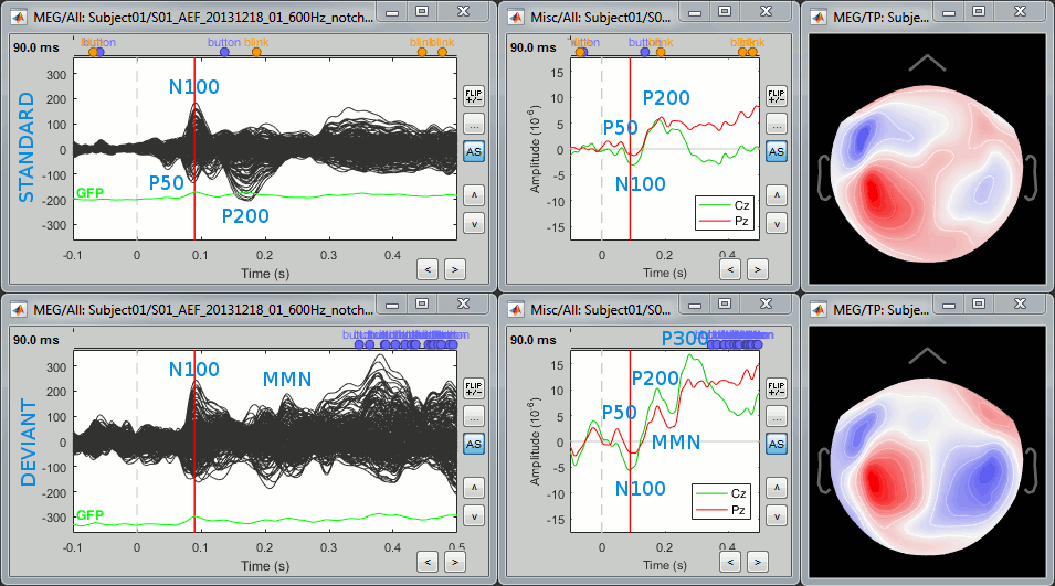
The legend in blue shows names often used in the EEG ERP literature:
P50: 50ms, bilateral auditory response in both conditions.
N100: 95ms, bilateral auditory response in both conditions.
MMN: 230ms, mismatch negativity in the deviant condition only (detection of an abnormality).
P200: 170ms, in both conditions but much stronger in the standard condition.
P300: 300ms, deviant condition only (decision making in preparation of the button press).
- Some seem to have a direct correspondence in MEG (N100) some don't (P300).
Additional quality check with the event markers:
- The standard average shows two unwanted events between 100ms and 200ms post-stimulus, one "blink" and one "button" response. The trials that contain them should be marked as bad and the average recomputed, because the subject is probably not doing the task correctly.
- We will not do this here because the SNR is high enough anyway, but remember that this option "Keep all events" from the averaging process provides a good summary of the recordings and can help you identify some bad trials.
Averaging bad channels
The bad channels can be defined independently for each trial, therefore we can have different numbers of data points averaged for different electrodes. If we have a channel A considered good for NA trials, the corresponding channel in the average file is computed in this way: sum(NA trials) / NA.
In the average file, a channel is considered good if it is good in at least one trial, and considered as bad if it is bad in all the trials. The entire file is then considered as if it were computed from the maximum number of good trials: Nmax = max(Ni), i=1..Ntrials.
This procedure allows the conservation of the maximum amount of data. However it may cause some unwanted effects across channels: the SNR might be higher for some channels than others. If you want to avoid this: mark the channels as bad in all the trials, or report all the bad channels to the average file. This can be done easily using the database explorer, see tutorial Bad channels.
Averaging across runs
As said previously, it is usually not recommended to average MEG recordings in sensor space across multiple acquisition runs because the subject might have moved between the sessions. Different head positions were recorded for each run, so we will reconstruct the sources separately for each each run to take into account these movements.
However, in the case of event-related studies it makes sense to start our data exploration with an average across runs, just to evaluate the quality of the evoked responses. We have seen in tutorial #4 that the subject almost didn't move between the two runs, so the error would be minimal.
Let's compute an approximate average across runs. We will run a formal average in source space later.
To run the same process again with different parameters: File > Reload last pipeline. Select:
By trial group (subject average): One average per experimental condition, across acquisition runs
Arithmetic average + Standard error: Save the standard error across all the trials in the same file
Keep all the event markers: Select this option, we are interested in the button press events.
The two averages are saved in the folder "Intra-subject". This is where all the results of processes involving multiple folders, within one subject, will be saved.
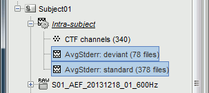
Standard error
If you computed the standard deviation or the standard error together with an average, it will be automatically represented in the time series figures.
Double-click on one of the AvgStderr files to display the MEG sensors.
The light-grey area around the sensors represent the maximum standard error around the maximum and minimum values across all the sensors.- Delete the useless events (cardiac and saccade).
Select two sensors and plot them separately (right-click > Channels > View selected, or "Enter").
The green and red areas represent, at each time point, the standard error around the signal.
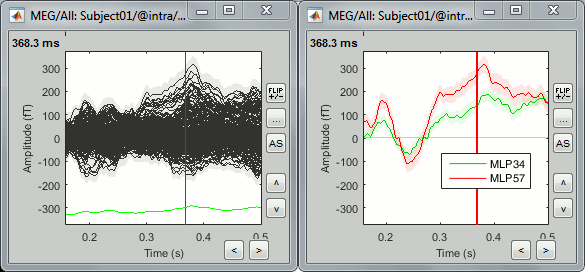
Number of trials
You should always be careful when comparing averages computed from different numbers of trials. In most cases, you can safely include all the trials in your averages, even in the case of imbalanced designs. However, for very low numbers of trials or when comparing peak amplitudes, having the same number of trials becomes more critical. See the following references for more details:
Luck SJ (2010)
Comparing conditions with different numbers of trialsThomas DG, Grice JW, Najm-Briscoe RG, Miller JW (2004)
The influence of unequal numbers of trials on comparisons of average event-related potentials
Selecting equal numbers of trials
If you decided you want to use the same number of trials across all the experimental conditions and/or across all the subjects, you can use a process to select them easily from the database.
Drag and drop all the "standard" and "deviant" trials for both runs in Process1.
Select the process "Files > Select uniform number of trials".
Select the options: By trial group (folder) and Uniformly distributed.
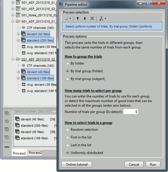
If you click on [Run], it doesn't do anything but highlighting the first selected file in the database explorer. This process just performs a file selection, it needs to be followed by another process that uses the selected files for computing something. However, you can see what was done in the process report. The reports are displayed only when an error or a warning was reported, but you can open them manually to check for additional messages. Menu File > Report viewer.
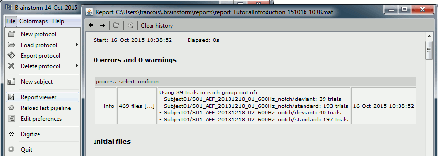
The comment in the report shows the 4 groups of trials that were identified based on the option we selected (group "by trial group and folder"), with the number of good trials per group.
The process picked 39 trials in each group, uniformly distributed in the list of available trials.
Example of trial indices selected for Run01/standard: [1, 6, 11, 16, 21, 26, 31, 36, ..., 188, 193]To average these selected trials together, you would just need to add the process "Average > Average files" after this selection process in the pipeline editor.
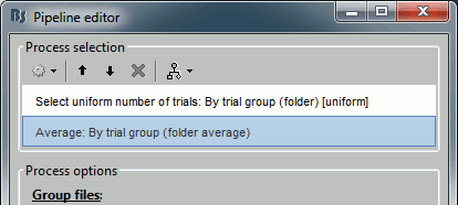
Process options
Available options in the process: File > Select uniform number of trials.
By folder: Groups by subject and by folder, ignoring the trial groups.
Here, it would identify two groups, one for each acquisition run: Run01, Run02.By trial group (folder): Groups by set of trials with the same name, separately for each folder and each subject. Here it would identify four groups: Run01/deviant, Run01/standard, Run02/deviant, Run01/standard.
By trial group (subject): Groups by set of trials with the same name, for each subject. The separation in folders is ignored. Here it would identify two groups: deviant, standard.
How many trials to select in each group:
Number of trials per group: This number of trials must be available in all the groups. If set to 0, the group with the lowest number of good trials is identified and the same number of trials is selected from all the other groups.
How to select trials in a group that contains more than the requested number (Nf files, selecting only Ns):
Random selection: Select a random subset of Ns trials. Trial indices: randperm(Nf,Ns)
First in the list: Select the first Ns trials. Trial indices: 1:Ns
Last in the list: Select the last Ns trials. Trial indices: Nf-Ns+1:Nf
Uniformly distributed: Select Ns equally spaced trials. Trial indices: round(linspace(1, Nf, Ns)))
On the hard drive
The average files have the same structure as the individual trials, described in the tutorial Import epochs.
Differences with the imported epochs
F: [Nchannels x Ntime] average recordings across all the trials, in Volts.
Std: [Nchannels x Ntime] standard error or standard deviation across all the trials, in Volts.
Leff: Effective number of averages = Number of good trials that were used to compute the file
Tutorial 17: Visual exploration
Authors: Francois Tadel, Elizabeth Bock, Sylvain Baillet
This tutorial illustrates the options Brainstorm offers to represent graphically and explore interactively the evoked responses we computed in the previous tutorial. It shows how to produce spatial maps of the sensors, temporal averages, save screen captures and movies.
Contents
2D/3D topography
The sensor values at one time instant can be represented on a surface. Each amplitude value gets associated with a color using a colormap (described in the next tutorial). We call this type of representation "sensor topography", it shows the spatial distribution of the magnetic fields (or electric potentials).
Show the MEG signals for the standard average in Run#01 (double-click on the file). This gives us a direct feedback of the current time instant and allows to jump quickly to a different time.
Right-click on the same file > MEG > select the menus: 3D sensor cap, 2D sensor cap, 2D disc.
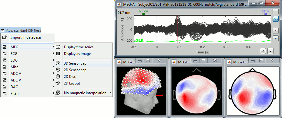
3D sensor cap: Represents the real 3D positions of the sensors.
2D sensor cap: The sensors are projected on a 2D plane. Realistic distribution of the sensors.
2D disc: The sensors are projected on a sphere, then displayed as flat disc. Sometimes distorted...
In each of these views, you can add markers to indicate the sensors and their labels.
Right-click on the figure > Channels > Display sensors/labels (or Ctrl+E).You can change the number of contour lines: Right-click > Contour lines > 0-20.

- In the 3D view, you can notice a hole in the right-occipital area. It corresponds to a damaged sensor in the MEG system we used for collecting this dataset.
For EEG/sEEG/ECoG recordings, there is an additional representation mode available:
"3D Electrode". This will be detailed in the advanced tutorials corresponding to these modalities.

Magnetic interpolation
By default, some of the views re-interpolate the fields that are recorded by the MEG sensors to get smoother displays. A simple inverse problem and forward problem are solved to reconstruct the magnetic fields on a high-resolution surface of virtual magnetometers (function channel_extrapm.m).
On Elekta-Neuromag systems, this interpolation has the effect of converting the topographies of the planar gradiometers into topographies of magnetometers, which deeply affects the display.
The menu "No magnetic interpolation" offers the same views, but without using this reconstruction of the magnetic field. A spatial interpolation of the values between the sensors is performed instead.
2D Layout
The menu 2D Layout represents, in the same figure, the spatial information (the values for each channel is represented where the sensor is actually located) and the temporal information (instead of just one single value, we represent the signal around the current time).
The light gray lines represent the zero amplitude (horizontal) and the current time (vertical lines).
To zoom in/out in each small graph, use the buttons at the bottom-right corner of the figure, or the corrsponding mouse shortcuts: Ctrl+mouse wheel and Shift+mouse wheel. To select multiple sensors simultaneously: right-click and move your mouse to enlarge the selection rectangle.
You can use this display mode to compare multiple files:
Select multiple files in the database explorer, right-click on any of them > 2DLayout.
Display as image
The menu "Display as image" shows the same information as the "time series" view, but the values for each sensor are represented with a color instead of a line.
Time selection
Click somewhere on the white part of the time series figure, hold the mouse button, and drag your mouse left or right: A transparent blue rectangle appears to represent the time selection. If you right-click on the figure, new options become available in the popup menu:
Set current time: Move the time cursor where the right-click occurred. The shortcut Shift+Click can be useful when trying to move in time on dense displays in columns view.
Set selection manually: Type the beginning and end of the selected window (in milliseconds).
Average time: Average over the selected time window and save it as a new file in the database.
Note that the best way to do this is to run the process "Average > Average time".Export to database: Extract the recordings and save them in a new file in the database.
If some sensors are selected, only their values are extracted, all the others are set to zero.
Note that the best way to do this is to run the process "Extract > Extract time".Export to file: Same, but in a user-defined file (not in the database).
Export to Matlab: Same, but export the selection as a variable in the current Matlab workspace.
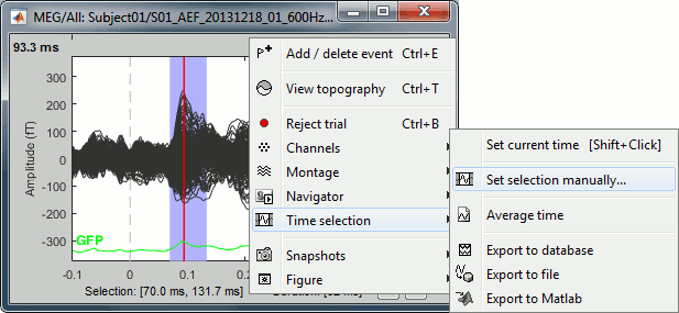
Snapshots
Using Brainstorm, you will quickly feel like saving the beautiful images you produce. Your operating system already provides some nice tools for doing this. Many other options are available in the "Snapshot" menu, accessible with a right-click on any Brainstorm figure.
Operating system
Windows/Linux: Press the PrintScreen key on your keyboard and paste the copied screen in your favorite image or text editor. The combination Alt+PrintScreen only copies the figure that is currently selected.
MacOS: Many more options available, Google for the best ones (see example).
Snapshot menu
The options available in the Snapshot menu depend on the type of data represented. Examples:
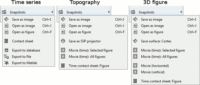
Save as image: Save the figure in a file, without the title bar and borders. Many formats available.
Open as image: Capture the figure and open it in as an image. This can be useful if you want to visually compare the selected figure with another one that you cannot display at the same time (because they have different time or frequency definitions).
Open as figure: Similar, but copies the figure as a new Matlab figure with some interactivity.
Contact sheet and movies: See next section.
Export to database: Save the recordings in the figure as a new entry in the database.
If there are selected channels, only their values will be saved, the others being set to zero.Export to file: Extract the time series displayed in this figure (or only the selected sensors), and save them in a file. Several exchange file formats available for exporting to another program.
Export to Matlab: Same thing, but exports the structure in a variable of the Matlab workspace.
Save as SSP projector: Create an SSP projector that removes the current topography.
Save surface: Save the surface in a file, with the current modifiers applied (smooth, resect).
Movie studio
Movie (horizontal/vertical): Rotate spatially the 3D scene.
Movie (time): Selected figure: Create .avi movies to show the evolution of the selected figure.
The dimensions of the movie depend on the actual size of the figure on the screen.
Resize the figure to the appropriate dimensions for the movie before using this menu.- Zoom in/out (mouse wheel) and move the image (middle click+move) to give enough space to the time stamp that is added at the bottom-left of the rendered movie.
- Don't do anything else while rendering: the captured figure must be visible all the time.
Movie (time): All figures: Instead of capturing one figure only, it captures them all. Arrange your figures the way you want and create a movie of all your workspace at once.
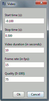
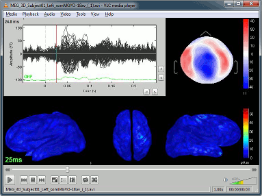
Contact sheets
A contact sheet is a large image representing many time frames of the same figure.
- Same recommendations as for movies: if you don't want the final image to be too big, reduce the size of the figure, zoom in, move, hide the colorbar. Keep the figure visible during the capture.
At the end, the image is displayed in an image viewer with which you can zoom (menu or wheel), move (click+move) and save the image (File > Save as).
Example for the standard average, run#01:
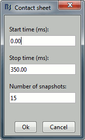
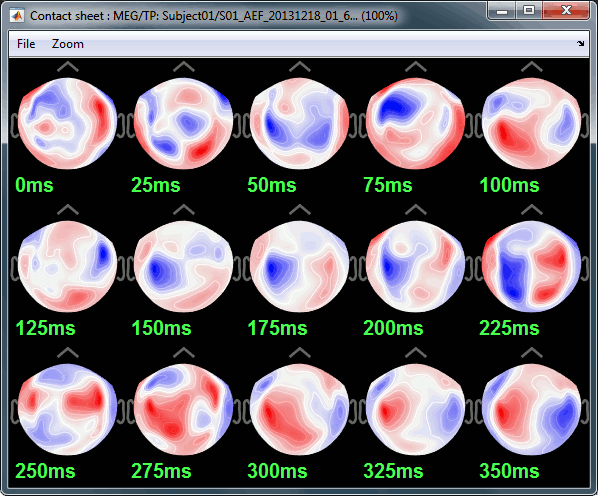
Edit the figures
All the figures can be edited with the Figure popup menu:
If you select both "Matlab controls" and "Plot edit toolbar", you will get all the tools available in the Matlab environment to explore the data and edit the figure. Select the button "Edit plot" to edit the graphic properties of an object (eg. select a signal, then right-click on it to edit its properties) or unselect it to get back to the regular Brainstorm figure interactivity.
Mouse shortcuts
Scroll
Mouse wheel: Zoom in / zoom out
Control + mouse wheel: Change the length of the displayed time window (2D Layout)
Control + mouse wheel: Vertical zoom (time series)
Click
Left click + move: Rotate (3D) or select (time)
Middle click + move: Move in zoomed figure (ie. panning)
Left click + right click + move: Move in zoomed figure (ie. panning)
Shift + left click: Force setting the current time, ignoring if a line was clicked (time series)
Right click + move: Vertical zoom (time series)
Right click + move: Select sensors (2D topography)
Right click: Popup menu
Double-click: Restore initial view
Click on something
Click on a line: Select a sensor
Shift + click on a line: Select a sensor and unselect all the others (2D topography)
Click on the colorbar + move: Change contrast (up/down) and brightness (left/right)
Keyboard shortcuts
Here is a memo of all the keyboard shortcuts for time series and topography figures. If you don't remember them, you can find most of them in the figure popup menus.
Arrows: Left, right, PageUp, PageDown: Move in time
Delete: Mark selected sensors as bad
Shift + Delete: Mark non-selected sensors as bad (=keeps ony the selected sensors)
Enter: View time series for the selected sensors
Escape: Unselect all the selected sensors
Shift + Escape: Set all the bad sensors as good (=brings back all the channels in the display)
Ctrl + A: Show axis on 3D figures (X,Y,Z)
Ctrl + B: Set trial as bad
Ctrl + D: Dock/undock figure in Matlab's figures list
Ctrl + E: Show sensors markers and labels (E=Electrode) or add an event marker (E=Event)
Ctrl + F: Copy figure, removes all the callbacks and detach from Brainstorm figure management
Ctrl + I: Save figure as image
Ctrl + J: Open figure as an image
Ctrl + R: Open Time series view (R=Recordings)
Ctrl + S: Open Sources view (S=Sources)
Ctrl + T: Open 2D sensor cap view (T=Topography)
Shift + letter: Change selected montage
F1, F2, F3: with or without Shift, calls the database navigator (F1=subject, F2=condition, F3=file)
1, 2, 3, 4, 5, 6, 7, 8, 9, 0: Set a pre-defined 3D view
+ / -: Increase/decrease the channel gain (vertical zoom for time series)
=: Apply view to all figures
*: Apply montage to all figures
- Notes for Mac users:
PageDown = Fn + DOWN
PageUp = Fn + UP
F1 = Fn + F1
Mouse wheel = Two finger up/down on the MacBook pad
Graphic bugs
If you observe any graphic problem with these displays, there might be an issue with the OpenGL drivers. You may try the following options.
- Update the drivers for your graphics card.
- Upgrade your version of Matlab.
Run the compiled version of Brainstorm (see Installation).
Turn off the OpenGL hardware acceleration: Menu File > Edit preferences > Software or Disabled.
- Send a bug report to the Mathworks.
Tutorial 18: Colormaps
Authors: Francois Tadel, Elizabeth Bock, Sylvain Baillet, Rana El Khoury Maroun
When displaying signals on the sensor array or on the cortex surface, we need to convert the amplitude of the signals into colors. The way the values are mapped to colors has a lot of influence on the visual interpretation of the figures. The selection of the appropriate colormap is an important step of the data exploration.
Contents
Colormap menus
Brainstorm keeps track of many user-defined colormaps: anatomy, EEG, MEG, sources, stat, time, time-frequency, etc. You can go to the Colormaps menu in the main window to see this list.
Usually, you will use only popup menus from specific figures to edit the colormaps.
Open a topography view for the standard average (right-click > MEG > 2D Sensor cap).
Right-click on the figure, you will only see the menu "Colormap: MEG recordings".
- If you modify a colormap, the changes will be applied to all the figures, saved in your user preferences and available the next time you start Brainstorm.
Standard color arrays
A colormap is an array of colors that are indexed and then mapped to values. It is represented by a [Nx3] matrix, where N is the number of colors available in it. Each color is coded with three values corresponding its relative levels of red, green and blue. In Matlab, the colors are coded between 0 and 1. To get an example, type "jet" in the Matlab command window, you will get the default values for the "jet" colormap.
We offer two ways of creating this array of colors in Brainstorm: you can use standard color arrays (modulated in contrast and brightness) or define your own.
Colormap name: The standard colormaps are referred to with names (bone, gray, jet, rwb, etc).
Pick a different color set in the menu to update all the figures with similar data types.
Brightness: Moves the center of the color array up and down. Example values: -80, 0, +80.
The term "brightness" is not well adapted for rbw, jet or hsv. It makes more sense for colormaps with only one tint that varies in intensity, such as the gray colormap. We use it here for lack for a better word.
Contrast: Changes the distance between the first and last colors. Example values: -80,0,+80.
You can modify these values by clicking directly on the color bar. Hold the mouse button, then:
Move up/down to change the brightness,
Move left/right to change the contrast.
Custom color arrays
To edit your own list of colors, use the menu "New..." at the end of the list of standard colormaps.
Open a 2D sensor cap view for the MEG sensors for the standard average (Run#01).
Right-click on the figure Colormap: MEG recordings > Colormap > New.Enter the name of the new colormap and the number of colors it will contain.
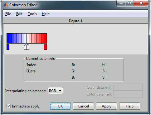
Each color in this color array is represented with a little square. The arrows in the the second row can be selected and deleted (delete key) or edited (double-click). They represent the key colors between which Matlab interpolates the other colors. Click on the second row to add more key colors.
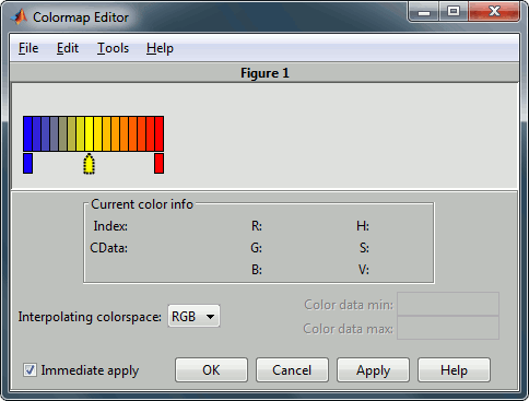
Once you are satisfied with your new colormap, click on [Ok].
It will update the figure. A new menu is now available in the list of colormap names.
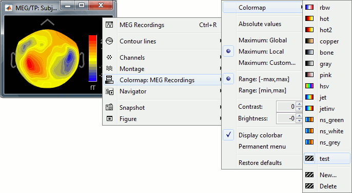
To delete the custom colormap currently selected, use the menu "Delete".
Color mapping
After defining the colors, we need to define how we want to map them with the values. The information necessary to do this color mapping is the value corresponding to the first and last colors. The color indices will be scaled linearly between these extrema.
Absolute values: Display the absolute values of the recordings, instead of the original values. This has the effect of constraining the color mapping to positive values only. It is not very useful for exploring the recordings: in EEG and MEG, the sign of the values is very important.
Maximum: Method used to estimate the minimum and maximum values of the colorbar.
Global: The bounds of the colormap are set to the extrema values found in the entire file.
Example: if you use the rbw colormap and the min and max values are [-200ft, +200ft], the colors will be mapped in the following way: -200ft is blue, +200ft is red, 0ft is white. The mapping is identical for all the time samples. If you select this option at t=0ms, the 2D topography figure will turn almost white because the average values are low before the brain response.Local: Uses the local min and max values at the current time frame AND for each figure, instead of the global min and max. Example: A t=0ms, the extrema values are roughly [-30ft, +30ft]. So the colors will be mapped in order to have: -30ft=blue and +30ft=red.
Custom: You can manually set the min/max bounds of the colorbar. It does not have to be symmetrical around zero. If you set the values to [-40,+20] ft, the white colors would correspond to values around -10ft, and values around 0ft would be displayed in pale red.

You can usually keep the option Local when looking at recordings, it is easier to read.
But keep in mind that it is not because you see flashy colors that you necessarily have strong effects. It's always a matter of colormap configuration.
Range: Use symmetrical or non-symmetrical colormaps.
[-max, max]: Symmetrical colorbar around the absolute value of the maximum.
Example: at t=170ms, the range is [-220ft, +90ft], the color mapping used is [-220ft, +220ft].[min, max]: Uses the real min and max. Useful for displaying values that are not centered on zero. Example: at t=170ms, the mapping used is [-220ft, +90ft], white is not zero.
This option is ignored when the option "Maximum: Custom" is selected.

Colormap management
Remember that when you change any of the options above, it is saved in your user preferences. If you close Brainstorm and start it again, the colormap configuration stays the same.
To reset the colormap to its default values:
Double-click on the color bar, or
Use the menu Restore defaults.
Two additional menus can help you manipulate the colormaps:
Display colorbar: In case you want to hide the color bar. Useful for contact sheets and movies.
Permanent menu: Open a window that displays this colormap sub-menu, for faster access.
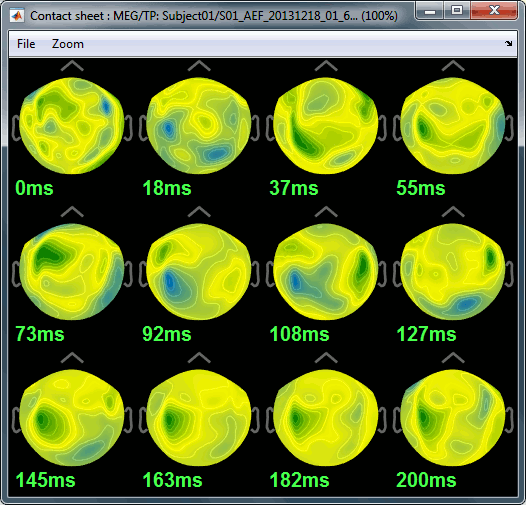
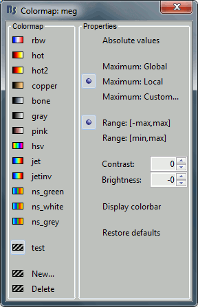
New default colormaps
Recently, the default colormaps of Brainstorm were changed because they lack important attributes of a good colormap: they don’t have linear lightness and they are not perceptually uniform. This can either cause details in the visualization to be hidden or create features that don’t exist in the underlying data, which results in a distortion of the perceived pattern. For that reason, new default colormaps were added to better represent the underlying data.
Here are the new colormaps created with their chosen names:
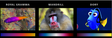
Three other colormaps were added: viridis and magma (taken from mpl colormaps) as well as a variation of viridis (viridis2). The colormaps were created using the viscm tool, which allows designing a colormap that has linear lightness and hue changes.
This paper presents the work done in more detail: colormap_optimization.pdf
JET Alternative
A new colormap created by Google, the Turbo colormap, was recently added. It is presented as a an improved rainbow colormap that can be used as an alternative to the popular JET colormap, resulting in a perceptually linear colormap.
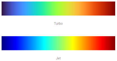
More information can be found on the following Google Blog post: https://ai.googleblog.com/2019/08/turbo-improved-rainbow-colormap-for.html
Tutorial 19: Clusters of sensors
Authors: Francois Tadel, Elizabeth Bock, Sylvain Baillet
In EEG, most of the analysis can be done directly on the electrode values. This tutorial explains how to group sensors in a cluster and overlay channels from different conditions in the same graph.
In MEG, we tend to avoid working at the sensor level because the signals are ambiguous, we work mostly in the source space, which is the topic of the next tutorials. If you are planning to work only with MEG recordings, you may skip this tutorial.
Contents
Cluster tab
The Cluster tab is not shown by default in the Brainstorm interface.
Click on the [+] button next to the Scout tab > Add: Cluster.
If the list of tabs is too busy, you can close some of them in the same way.

The Cluster tab is similar to the Scout tab, but much simpler. It contains a toolbar to create and edit clusters, a list of existing clusters and a few display options at the bottom.
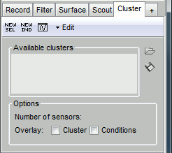
[NEW SEL]: Create a cluster containing the channels that are currently selected in the interface.
[NEW IND]: Create a cluster with channels selected by index, name or type.
[Display clusters time series]: Shows the time series of the selected clusters for all the files that are currently open in the interface.
Edit: Menus to modify the selected clusters.
Creating clusters
A cluster is a group of one or multiple channels. There are two ways for creating a new one.
Display the MEG recordings for the standard average of Run#01 (double-click on the file).
Add a 2D topography (Ctrl+T), display the sensors and select a group of them (right-click+move).

In the Cluster tab, click on [NEW SEL]. It creates a new cluster "c1".
Double-click on it to rename it to "cmax" (or menu Edit > Rename).In the Cluster tab, click on [NEW IND]. Enter the name of the sensor "MLT12". Rename it to "cmin".
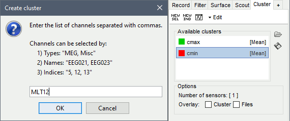
Selection: When you change the selected cluster in the list, it selects the corresponding sensors in all the figures. The number of channels involved in the selection is displayed at the bottom of the tab. You can select multiple clusters at once, holding the Ctrl/Shift/Command button while clicking.
Saving: The clusters are saved in the channel file. When you close all the figures relative to a dataset, it prompts for saving the modifications in the channel file. When opening again the dataset, the Cluster tab will open automatically to show the saved clusters.

Displaying clusters
We now have two clusters available in the list. The second one contains only one channel, displaying it corresponds to displaying the channel time series. The first one contains multiple channels, we need to apply a function to group them into one signal only.
The cluster function used to group multiple signals into one is shown on the right of the cluster list. By default it uses a simple average ("Mean"). You can edit this cluster function with the menu Edit > Set cluster function.
Select one cluster and click on the [Display cluster] button (third from the left in the toolbar).
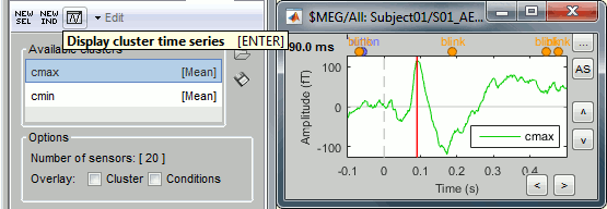
Select the two clusters at once and click on [Display cluster] again.
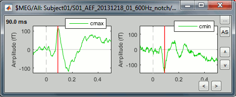
To have the two signals in the same graph, select the option "Overlay: Cluster". Click on [Display].

In the database explorer: Double-click on the deviant average of the same run.
Click on [Display cluster] again, now it displays the clusters values for both conditions.

Unselect "Overlay: Cluster" and select "Overlay: Files". If both conditions are selected in the database explorer and both clusters are selected in the Cluster tab, it will group the signals in a different way: one graph per cluster, each one showing the two condition averages.

From the database explorer
Once the clusters are defined, you can apply them to any number of files in the database in one click.
- Close all the figures with the [X] button in the top-right corner of the Brainstorm figure.
In the Cluster tab, select only one of the two clusters, select Overlay: Files.
In the database explorer, select all the averages for both runs. Right-click on one of the selected files > Clusters time series. On this graph, you can verify that the selected cluster behaves in the same way in the two acquisition runs.
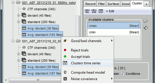
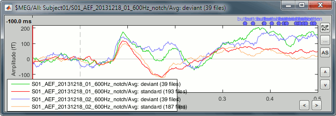
Processes
Extract > Clusters time series: The process computes the clusters signals and save them in a new file in the database. Select the files of interest in Process1, and select the option "Concatenate" if you want the cluster signals from all the input files to be saved in the matrix file. If the option is not selected, the process creates one new matrix file for each input file.
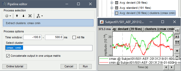
Import > Channel file > Import clusters of channels: The process allows to automate the loading of the same clusters for multiple datasets. In Process1, select at least one data file in each folder in which you want to import the clusters (it will only add it once per channel file, even if you have many data files from the same folder in input), then select the cluster file to import. This cluster file can be generated from the Cluster tab: select one or more clusters and click on the [Save] button.

Scripting
The function db_set_clusters.m allows adding clusters to multiple channels programmatically. Read the header of the function for help with the parameters. Here are some examples:
Add the clusters defined in array of structures 'sClusters' to the channel file of folder pointed by iStudy:
db_set_clusters([], iStudy, sClusters);
Copy all the clusters from a channel file to all the other channel files in the same subject:
db_set_clusters(ChannelFile, 'AllConditions');
Remove all the clusters from all the channel files in the database.
db_set_clusters([], 'AllSubjects', []);
Get a structure template for sCluster:
sCluster = db_template('cluster');Copy the clusters selected in the Clusters tab of the Brainstorm figure to specific studies:
panel_cluster('CopyClusters', iStudies);
Tutorial 20: Head modeling
Authors: Francois Tadel, Elizabeth Bock, John C Mosher, Richard Leahy, Sylvain Baillet
The following tutorials describe how cerebral currents can be estimated from the MEG/EEG recordings we have processed so far. To achieve this, we need to consider two distinct modeling problems: the modeling of the electromagnetic properties of the head and of the sensor array (a.k.a. head model or forward model), and the estimation of the brain sources which produced the data, according to the head model in question. That second step is known as source modeling or solving an inverse problem. It requires that forward modeling of head tissues and sensor characteristics is completed first. This tutorial explains how to compute a head model for the participant to the auditory oddball experiment.
Contents
Why estimate sources?
Reconstructing the activity of the brain from MEG or EEG recordings involves several sophisticated steps. Although Brainstorm simplifies the procedures, it is important to decide whether source modeling is essential to answer the neuroscience question which brought you to collect data in the first place.
If one of your primary objectives is to identify and map the regions of the brain involved in a specific stimulus response or behavior, source estimation can help address this aspect. Empirical interpretations of sensor topographies can inform where brain generators might be located: which hemisphere, what broad aspect of the anatomy (e.g., right vs. left hemisphere, frontal vs. posterior regions). Source estimation improves anatomical resolution further from the interpretation of sensor patterns. The spatial resolution of MEG and EEG depends on source depth, the principal orientation of the neural current flow, and overall SNR: still, a sub-centimeter localization accuracy can be expected in ideal conditions, especially when contrasting source maps between conditions in the same participant. As for other imaging modalities, spatial resolution of group-level effects (i.e. after averaging across multiple participants) is limited by the accuracy of anatomical registration of individual brain structures, which are very variable between participants, and intersubject variations in functional specialization with respect to cortical anatomy.
Source mapping is a form of spatial deconvolution of sensor data. In EEG in particular, scalp topographies are very smooth and it is common that contributions from distant brain regions overlap over large clusters of electrodes. Moving to the source space can help discriminating between contributing brain regions.
In MEG, source maps can be a great asset to alleviate some issues that are specific to the modality. Indeed in MEG and contrarily to EEG, the head of the participant is not fixed with respect to sensor locations. Hence data sensor topographies depend on the position of the subject's head inside the MEG sensor array. Therefore, between two runs of acquisition, or between subjects with different head shapes and sizes and positions under the helmet, the same MEG sensors may pick up signals from different parts of the brain. This problem does not exist in EEG, where electrodes are attached to the head and arranged according to standard positions.
Another important point to consider when interpreting MEG sensor maps and that can be solved by working in the MEG source space instead, is that MEG manufacturers use different types of sensor technology (e.g., magnetometers vs. gradiometers; axial vs. tangential gradiometers, etc. yielding different physical measures). This is not an issue with EEG, with essentially one sensor type (electrodes, dry or active, all measuring Volts).
Nevertheless, if your neuroscience question can be solved by measuring signal latencies over broad regions, or other aspects which do not depend crucially on anatomical localization (such as global signal properties integrated over all or clusters of sensors), source modeling is not required. To sort out this question will influence the time and computational resources required for data analysis (source analysis multiplies the needs in terms of disk storage, RAM and CPU performance).
The origins of MEG/EEG signals
To better understand how forward and inverse modeling work, we need to have a basic understanding of the physiological origins of MEG/EEG signals. Note that, as always with modeling, we need to deal with various degrees of approximation.
Overall, it is assumed that most of - but not exclusively - the MEG/EEG signals are generated by postsynaptic activity of ensembles of cortical pyramidal neurons of the cerebral cortex. The reason is essentially in the morphology and mass effect of these cells, which present elongated shapes, and are grouped in large assemblies of cells oriented in a similar manner approximately normal to the cortex. Mass effects of close-to-simultaneous changes in post-synaptic potentials across the cell group add up in time and space. These effects can conveniently be modeled at a mesoscopic spatial scale with electric dipoles distributed along the cortical mantle (green arrows in figure below). Note that there is growing evidence that MEG and EEG are also sensitive to deeper, cortical and subcortical structures, including brain nuclei and the cerebellum. Brainstorm features advanced models of these structures, as an option to your analysis. The emphasis in this tutorial is on cortical source models, for simplicity.
The primary and volume currents generated by current dipoles create differences in electrical potentials and magnetic fields that can be detected outside the head. They can be measured with electrodes placed on the skin (EEG, with respect to a reference) or very sensitive magnetic detectors (MEG).
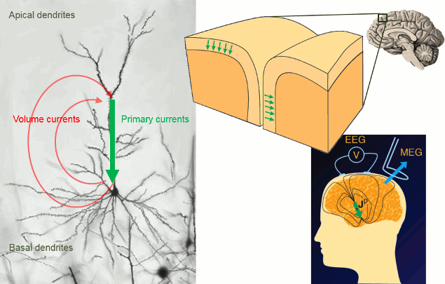
Source models
Dipole fitting vs distributed models
MEG/EEG source estimation consists in modeling brain activity with current dipoles. A current dipole is a convenient model equivalent to the net post-synaptic electrophysiological activity of local assemblies of neurons. Two main approaches have been explored for source MEG/EEG estimation: dipole fitting methods - where the position and amplitude of one to a few equivalent current dipoles (ECD) are estimated over relatively short time windows - and distributed models - where the location (and typically, the orientation) of a large number dipoles is fixed; the dipoles sample a spatial grid covering the entire brain volume or the cortical surface - requiring estimation of the amplitude of a vast number of dipoles in a fixed grid at each time point.
Equivalent dipole fitting approaches are quite straightforward and can be adequate when the number of brain regions expected to be active is small (ideally only one). Therefore, it is most adequate for responses at early post-stimulus latencies. They cannot generalize to capture complex dynamics over extended period of time (epochs) and the associated estimation techniques are quite sensitive to initial conditions (how many dipoles to fit? where does the search start? etc). Our strategy in Brainstorm is to promote distributed source models, which are less user dependent, can generalize to all experimental conditions, and yield time-resolved image volumes that can be processed in many different, powerful ways (group statistics, spatial segmentation, use of regions of interest, correspondence with fMRI, etc.)
Source constraints
When opting for distributed source models, the positions and orientations of the elementary dipoles that will define the "voxel" grid of the source images produced need to be defined. This set of dipoles is called the source space.
By default, Brainstorm constrains the source space to the cortex surface, where signal-to-noise and sensitivity is maximum in MEG/EEG. Note however that more complete models that include subcortical structures and the cerebellum are available in Brainstorm. Therefore, one decision you need to make before proceeding with source imaging is whether more complete source spaces are required to answer your neuroscience question.
For this tutorial, we use the simple approach where current dipoles are automatically assigned to each of the vertices of the cortical surface (see the nodes in the grey mesh in the leftmost image below). When importing the anatomy of the subject, we downsampled the cortex surface to 15,000 vertices.
This default number of 15,000 vertices is empirical. In our experience, this balances the adequate geometrical sampling of cortical folds with the volume of data to be analyzed. To use a smaller number of vertices (sources) oversimplifies the shape of the brain; to use more vertices yields considerably larger data volumes, without necessarily adding to spatial resolution, and may lead to practical hurdles (CPU and memory issues.)
Orientation constraints
After defining the locations of the dipoles, we also need to define their orientations. Brainstorm features two main options: unconstrained dipole orientations or orientations constrained perpendicularly with respect to the cortical surface.
In the unconstrained case, three orthogonal dipoles are assigned to each vertex of the cortex surface. This triplet can account mathematically for local currents flowing in arbitrary directions. The total number of elementary sources used in that case amounts to 45,000 dipoles (3 orientations x 15,000 vertices).
In the constrained case, one dipole is assigned to each vertex with its orientation perpendicular to the cortical surface. The benefit to this option is that it restricts the number of dipoles used to 15,000 (one per vertex). Results are also easier to process and visualize. However, there are some instances where such constraint is exaggerated and may bias source estimation, for instance when the individual anatomy is not available for the participant.
In the Brainstorm workflow, this orientation constraint is offered as an option of the inverse model and will be discussed in the following tutorial sections. In the present tutorial, we compute the forward model corresponding to a grid of 15,000 cortical sources without orientation constraints (hence a total of 45,000 dipoles). Note that the orientation constraint can be applied subsequently in the workflow: We do not have to take such hard decision (constrained vs. unconstrained source orientation) at this stage.
Whole-brain model
The constraint of restricting source locations to the cortical surface can be seen as too restrictive in some cases, especially if subcortical areas and cerebellum are regions of interest to the study. Brainstorm features the possibility to use the entire brain volume as (volume) source space (see green dots below: they represent dipole locations sampling the entire brain volume). One minor drawback of such model is that the results produced are impractical to review. We encourage users interested in more sophisticated approaches to add non-cortical structures to their MEG/EEG model to consult the sections concerning Volume and Mixed Head Volumes in the advanced tutorials about source modeling.
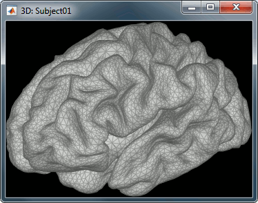
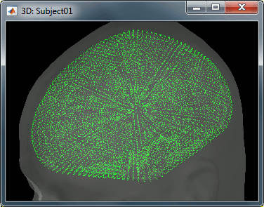
Forward model
We now need to obtain a model that explains how neural electric currents (the source space) produce magnetic fields and differences in electrical potentials at external sensors (the sensor space), given the different head tissues (essentially white and grey matter, cerebrospinal fluid (CSF), skull bone and skin).
The process of modeling how data values can be obtained outside of the head with MEG/EEG from electrical current dipoles in the brain is called forward modeling or solving a forward problem.
In Brainstorm, we call the outcome of this modeling step a "head model", a.k.a. forward model, leadfield matrix or gain matrix in the MEG/EEG literature.
In this tutorial we will use the default source space: a lower-resolution cortical surface representation, with 15,000 vertices, serving as location support to 45,000 dipoles (see above: models with unconstrained orientation). Note that we use the terms dipole and source interchangeably.
We will obtain a matrix [Nsensors x Nsources] that relates the activity of the 45,000 sources to the sensor data collected during the experiment.

Available methods for MEG forward modeling
Single sphere: The head geometry is simplified as a single sphere, with homogeneous electromagnetic properties.
Overlapping spheres: Refines the previous model by fitting one local sphere under each sensor.
OpenMEEG BEM: Symmetric Boundary Element Method from the open-source software OpenMEEG. Described in an advanced tutorial: BEM head model.
DUNEuro FEM: Finite Element Method from the open-source software DUNEuro. Described in an advanced tutorial: FEM head model
Models recommended for each modality
MEG: Overlapping spheres.
Magnetic fields are less sensitive to heterogeneity of tissue in the brain, skull and scalp than are the scalp potentials measured in EEG. We have found that this locally fittedspheres approach (one per sensor) achieves reasonable accuracy relative to more complex BEM-based methods: [Leahy 1998], [Huang 1999].EEG: OpenMEEG BEM.
Since EEG measures differential electric potentials on the scalp surface it depends on the effects of volume conduction (or secondary currents) to produce the signals we measure. As a result EEG is very sensitive to variations in conductivity not only in the tissue near the brain's current sources but also with the skull and scalp. Some tissues are very conductive (brain, CSF, skin), some are less (skull). A realistic head model is advised for integrating their properties correctly. When computing a BEM model is not an option, for instance if OpenMEEG crashes for unknown reasons, then Berg's three-layer sphere can be an acceptable option.sEEG/ECoG: The OpenMEEG BEM option is the only model available for this data modality.
Computation
The forward models depend on the anatomy of the subject and characteristics of EEG/MEG sensors: the related contextual menus are accessible by right-clicking over channel files in the Brainstorm data tree.
In the imported Run#01, right-click on the channel file or the folder > Compute head model.
Keep the default options selected: Source space=Cortex, Forward model=Overlapping spheres.
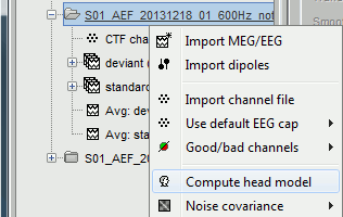
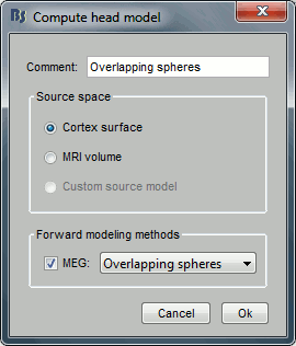
A new file will then appear in the database. Headmodel files are saved in the same folder as the channel file's.
This file is required for EEG/MEG source estimation: This next step will be described in details in the following tutorial sections.Right-click on the head model file > Check spheres. This window shows the spheres that were estimated to compute the head model. You can visualize and verify their location by following the indications written in green at the bottom of the window: use left/right arrows. At each step, the current sensor marker is displayed in red, and the sphere shown is the local estimation of the shape of the inner skull immediately below the sensor.
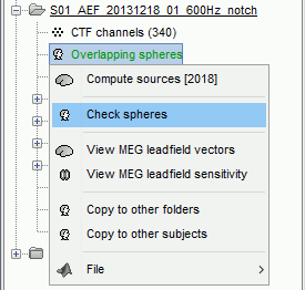
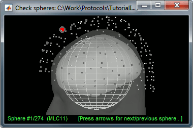
Although in principle, the overlapping-sphere method requires the inner skull surface, this data is not always available for every participant. If not available, a pseudo-innerskull surface is estimated by Brainstorm using a dilated version of the cortex envelope.
Repeat the same operation for the other file. We now have two different acquisition runs with two different relative positions of the head and of the sensors. We now need to compute two different head models (one per head/sensor location set).
In the imported Run#02, right-click on the channel file > Compute head model.
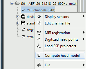
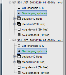
Forward Modeling: Qualitative Leadfield comparison
This page expands on the head modeling descriptions by providing a qualitative comparison of the forward model solutions across different scenarios <Qualitative Leadfield comparison>
Database explorer
This section contains additional considerations about the management of the head model files.
If multiple head models were computed in the same folder (e.g., after experimenting different forward models), one will be displayed in green and the others in black. The model in green is selected as the default head model: it will be used for all the following computation steps (e.g., source estimation). To change the default to another available head model, double-click on another head model file (or right-click over that file > Set as default head model).
You can use the database explorer for batching the computation of head models (across runs, subjects, etc.). The "Compute head model" item is available in contextual menus at multiple instances and all levels of the database explorer. The same forward model type is obtained recursively, visiting all the folders contained in the selected node(s) of the database explorer.
On the hard drive
Right-click on any head model entry > File > View file contents:
Structure of the head model files: headmodel_*.mat
MEGMethod: Type of forward model used for MEG sensors ('os_meg', 'meg_sphere', 'openmeeg' or empty).
EEGMethod: Type of forward model used for EEG sensors ('eeg_3sphereberg', 'openmeeg' or empty).
ECOGMethod: Type of forward model used for ECoG sensors ('openmeeg' or empty).
SEEGMethod: Type of forward model used for sEEG sensors ('openmeeg' or empty).
NIRSMethod: Type of forward model used for NIRS sensors.
Gain: Leadfield matrix, [Nsensors x Nsources] (in practice, equivalent to [Nsensors x 3*Nvertices]).
Comment: String displayed in the database explorer to represent this file.
HeadModelType: Type of source space used for this head model ('surface', 'volume', 'mixed').
GridLoc: [Nvertices x 3], (x,y,z) positions of the grid of source points. In the case of a surface head model, it corresponds to a copy of the 'Vertices' matrix from the cortex surface file.
GridOrient: [Nvertices x 3], directions of the normal to the surface for each vertex point (copy of the 'VertNormals' matrix of the cortex surface). Empty in the case of a volume head model.
GridAtlas: In the case of mixed head models, contains a copy of the "Source model options" atlas structure that was used for creating the model.
SurfaceFile: Relative path to the cortex surface file related with this head model.
Param: In case of a surface head model, it contains a description of the sphere that was estimated for each sensor (Center/Radius).
History: Date and brief description of the method used for computing the head model.
Gain matrix
The Gain matrix is the most important piece of information in the structure. It stores the leadfields for 3 orthogonal orientations (x,y,z) at each grid point (p1, p2, etc). The information relative to each pair sensor <-> grid source point is stored as successive columns of the matrix are ordered as: [p1_x, p1_y, p1_z, p2_x, p2_y, p2_z ...]. For the tutorial introduction dataset, with 15002 sources, the gain matrix has 45006 columns.
To convert this unconstrained leadfield matrix to that of an orientation-constrained model, where the orientation of each dipole is fixed and normal to the cortex surface:
Export the head model file to the HeadModel structure: Right-click > File > Export to Matlab.
At the Matlab prompt:
> Gain_constrained = bst_gain_orient(HeadModel.Gain, HeadModel.GridOrient);The dimension of the output matrix is three times smaller (now only one source orientation at each location): [Nsensors x Nvertices]
Useful functions
in_bst_headmodel(HeadModelFile, ApplyOrient, FieldsList): Read contents of the head model file.
bst_gain_orient(Gain, GridOrient): Apply orientation constraints.
Additional documentation
Articles
Mosher, Leahy RM, Lewis PS
EEG and MEG: Forward solutions for inverse methods
IEEE Trans Biomedical Eng, 46(3):245-259, Mar 1999Leahy RM, Mosher JC, Spencer ME, Huang MX, Lewine JD (1998)
A study of dipole localization accuracy for MEG and EEG using a human skull phantom
Electroencephalography and Clinical Neurophysiology, 107(2):159-73Huang MX, Mosher JC, Leahy RM (1999)
A sensor-weighted overlapping-sphere head model and exhaustive head model comparison for MEG
Phys Med Biol, 44:423-440Gramfort A, Papadopoulo T, Olivi E, Clerc M
OpenMEEG: opensource software for quasistatic bioelectromagnetics
BioMedical Engineering OnLine 45:9, 2010
Tutorials and forum discussions
Tutorial: BEM with OpenMEEG
Tutorial: Volume source estimation
External documentation: Electromagnetic neural source imaging
Forum: Sensor modeling: http://neuroimage.usc.edu/forums/showthread.php?1295
Forum: EEG reference: http://neuroimage.usc.edu/forums/showthread.php?1525#post6718
Forum: EEG and default anatomy: http://neuroimage.usc.edu/forums/showthread.php?1774
Forum: Mixed head models indices: http://neuroimage.usc.edu/forums/showthread.php?1878
Forum: Gain matrix units for EEG: http://neuroimage.usc.edu/forums/showthread.php?1837
Tutorial 21: Noise and data covariance matrices
Authors: Francois Tadel, Elizabeth Bock, John C Mosher, Richard Leahy, Sylvain Baillet
Modeling and measuring certain characteristics of the noise contaminating the data is beneficial to source estimation. For instance, minimum norm estimators can integrate second-order sample statistics of sensor noise (summarized into a noise covariance matrix, see below). Beamformers further require similar sample statistics for the data portion of interest (summarized into a data covariance matrix). This first section of this tutorial explains how to obtain a noise covariance estimate from MEG empty room recordings.
Contents
Noise covariance
Instrumental noise ("sensor noise") can be readily captured in MEG using two or more minutes of empty room measurements. We encourage the use of noise recordings collected the same day as the subject's recordings (if possible just before the session) and pre-processed in the same manner (with same sampling rate and same frequency filters applied) as the participant data. In this study we have already prepared a 2-min segment of noise recordings that we will use to estimate noise covariance sample statistics.
Right-click on the entry for noise recordings > Noise covariance. Available menus:
Compute from recordings: Use the selected recordings to estimate noise covariance statistics.
No noise modeling: Use an identity matrix as noise covariance. This option is useful when no noise recording is available (e.g. ongoing EEG without any baseline of no interest).
Import from file: Use noise covariance statistics available from another source (e.g., obtained using the MNE software.)
Import from Matlab: Import any [Nchannels x Nchannels] matrix as noise covariance matrix from the Matlab workspace.
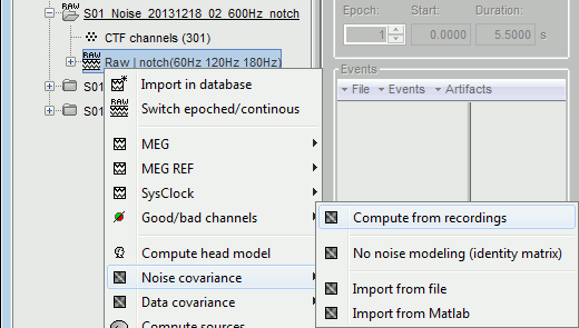
Select the menu Noise covariance > Compute from recordings. Available options:
Files: The top part of this window shows a summary of the files that have been selected to estimate the noise: 1 file of 120s at 600Hz. Total number of time samples in selected file: 72,000. We can also choose to use only a portion of this file, with the option "baseline". The large continuous files are split in blocks of a maximum of 10,000 samples that are then processed as different files.
Remove DC offset: All the selected blocks of data are baseline corrected and concatenated to form a large matrix "F". There are two options for baseline correction:
Block by block: The average value of each channel is subtracted from each block before concatenating files together. Let Fi contain data from block #i:
F = Concatenate[Fi - mean(Fi)].Global: The average value of each channel is removed after concatenation (same correction for all blocks): F = Concatenate[Fi] - mean(Concatenate[Fi]).
The sample noise covariance is computed from F: NoiseCov = F * F' / Nsamples
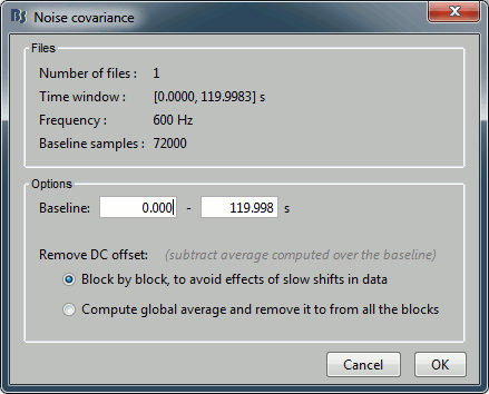
For this tutorial, keep the default options and click on [OK].
- One new file is created and appears under the noise data folder, next to the channel file. The corresponding contextual menus are:
Display as image: Opens a display of the noise covariance matrix as an indexed image (same as double-click on file). This can be useful to quickly control the quality of the recordings: for instance, noisier channels appear as rows/columns marked in red.
Copy to other folders: Copy the file obtained to all the other folders of the same subject, to avoid re-computing the noise covariance statistics again for each folder from the same session.
Copy to other subjects: Copy this file to all the folders of all the subjects in the protocol.
You can also copy a noise covariance file to another folder just like any other file:
Right-click > File > Copy/Paste, or keyboard shortcuts Ctrl+C/Ctrl+V.
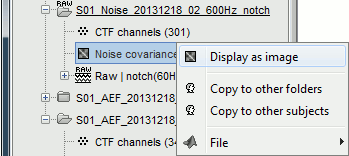
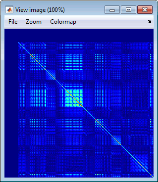
Right-click on the the noise covariance file > Copy to other folders: We need this file in the two folders where the epochs were imported before we compute the respective source models.
Variations on how to estimate sample noise covariance
The sample noise covariance matrix is straightforward to obtain. Brainstorm's interface features a lot of flexibility to select the files and time windows used to calculate the sample statistics. You need to have a clear understanding of the concept of "noise" to pick the best possible option. We support the notion that noise covariance accounts for contaminants that remain present in the data after preprocessing is complete. Hence it is not meant to account for eye blinks, heartbeats, muscle artifacts, flat or bad channels and noisy segments: all of these need to be taken care of during previous preprocessing steps, as show in previous tutorial sections. The noise covariance entry is to account for remaining and stationary instrumental, sensor and environmental noise components. For this reason, the ideal scenario is to use segments of recordings that contain exclusively this type of contaminant, or segments of recordings deemed not to contain any of brain signals of interest. This section is advanced reading material that can be used as a reference in a different experimental context.
The case of MEG
From empty-room recordings: actual noise measurements (due to the instrument, environment) using empty-room conditions (no subject under the MEG helmet) are possible in MEG. We recommend you obtain 2 to more minutes of empty-room data right before bringing the subject in the MEG room, or right after the experiment is finished.
You can verify quantitatively how stable and reproducible is the noise covariance estimated (e.g., during the day/week). The MEG system may be located in a "quiet environment", allowing that you re-use the same noise recordings and therefore, noise covariance matrix, for all runs and subjects acquired on the same day.
From resting-state segments: When studying evoked responses (aka event-related responses), you may want to collect a few minutes of recordings where the subject is resting, i.e. not performing the task. Using these segments to obtain the noise covariance estimates implies that resting brain activity will be assumed as "noise", which we know now is not the case. We therefore encourage MEG users to acquire short empty-room runs instead.
From pre-stimulus baseline: Using concatenated pre-stimulation baseline segments from individual trials is in principle similar to the previous scenario, hence has similar limitations: regions prominently active during pre-stimulation baseline will tend to be attenuated by source analysis.
The case of EEG
It is less straightforward to estimate sensor noise from EEG data, because the electrodes need to be attached to a conductive medium (i.e. the scalp) to produce signals. Therefore only the last two options shown above in the MEG section are possible in EEG:
resting baseline and pre-stimulation baseline.
EEG noise levels depend on the quality of the electrode connection with the skin. It varies considerably between subjects, and during acquisition. Indeed, the conductive gel/paste/solution used for contact tends to dry up, which affects impedance. The electrode cap/locations can also move slightly, depending on how cooperative the participants. To account for variable noise levels between subjects, it is therefore preferrable to use one channel file per subject, because it allows the definition of one noise covariance entry per participant. In some specific cases, if the quality of the recordings varies a lot over time, it is preferrable to segment long recordings into shorter runs, and obtain different noise covariance matrices for each.
EEG in resting-state conditions
If the target brain activity to your experiment is resting, resting segments cannot be used to obtain noise statistics. For MEG, use empty-room measurements as explained above. For EEG, there are possible options: use sensor variance estimates, or avoid estimating empirical noise statistics.
Option #1: Calculate noise covariance over a long segment of resting recordings, but save only the diagonal elements, i.e. the variance measured at each sensor. This option is available in Brainstorm's advanced options of source computation: select the option "Diagonal noise covariance".
Option #2: Select "No noise modeling" in the contextual menu. This option uses the identity matrix as noise covariance matrix, and therefore assumes equal, unit variance of noise on every sensor. In inverse modeling, this is equivalent to assuming that noise is homoskedastic, and equivalent on all sensors. With this latter option, if data quality is not even on all electrodes, a higher noise level on some sensors may be explained with stronger, spurious source activity.
Epilepsy
Interictal spikes are often considered as events of interest in epilepsy studies. In that respect, they can be considered as a form of brain activity evoked by the epileptogenic process, very much like a stimulus-related response. For this reason, one shall be cautious about how to define noise conditions from ongoing EEG or MEG recordings to study epilepsy. Defining a segment of time adjacent to the spike as "background noise" is certainly not justified. In practice, however, one often uses a data segment clear from visible interictal activity. As discussed above, MEG has the additional, preferred option of using empty-room data as a baseline - an option not available with EEG.
The same options as above are available to the epilepsy researcher:
Option #1a: Estimate noise covariance statistics from blocks of recordings away from the peak of any identified interictal spike, and keep only the diagonal (the variance of each sensor time series). This option is available in Brainstorm's advanced options of source computation: select the option "Diagonal noise covariance".
Option #1b: If a large period of time clear of visible interictal events is available, use this latter to estimate the full noise covariance array.
Option #2(MEG): Use empty-room data as baseline.
Option #3: Select "No noise modeling" in the popup menu (identity matrix, unit variance of noise on every sensor).
Recommendations
Long noise recordings: In order to obtain a more accurate estimation of the noise covariance, a sufficiently large number of time samples is required: at least N*(N+1)/2 samples, (N is the number of sensors.) This amounts to 40s of data for CTF275 recordings at 1000Hz, or 20s for 128-channel EEG at 500Hz. Remember to always use as much data as possible to estimate noise covariance statistics.
Do not use signal averages: For this reason, you should never compute the noise covariance matrix from averaged responses. If you want to import recordings that you have fully pre-processed with another program, we recommend you import the individual trials and use them to estimate noise covariance. If you can only import the averaged responses in Brainstorm, please be aware that you may under estimate noise levels and bias source results.
Using one block: If you want to use a segment of "quiet" recordings in a continuous file: right-click on the continuous file > Noise covariance > Compute from recordings, then copy the noise covariance to the other folders. This is the case described in this tutorial.
Use single trials: If you want to use the pre-stimulation baseline from single trials, first import the trials in the database, then select all the groups of imported trials at once, right-click on one of them > Noise covariance > Compute from recordings, and finally copy the file to the other folders.
Using multiple continuous blocks: This is similar to the single trial case. Import in the database all the blocks you consider as quiet resting baselines, then select all the imported blocks in the database explorer > Noise covariance > Compute from recordings.
Data covariance
Beamforming source mapping further requires the estimation of data covariance statistics. The LCMV beamformer uses an estimated data covariance matrix to compute spatial filters that define the beamformer. It is important that this covariance matrix contains contributions from all sources that contribute to the data over the time window to be analyzed (signal + noise).
We have found, as have others, that it is important to use a relatively long time window for robust beamformer performance. This also helps to avoid numerical instability when inverting the data covariance, as required in computing the beamformer kernel matrix. Our recommendations:
Evoked responses: Use a window that spans prestim through the end of the response of interest, with a minimum of 500ms total duration.
Spontaneous data: Use the full time window to be analyzed, with a minimum of 30s of data.
The procedure to compute the data covariance is very similar to the noise covariance:
For run#01, select all the trials, right-click > Data covariance > Compute from recordings.
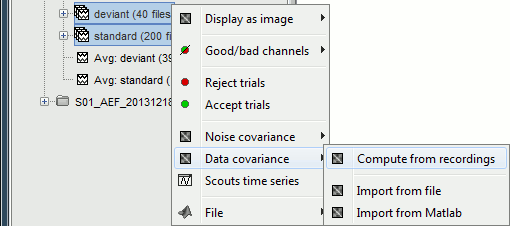
We need to specify two time windows:
Baseline: Pre-stimulus time, used for DC offset correction (subtracts the baseline mean).
Data: Time segment of interest (let's use all the time available post-stimulus in this tutorial example).
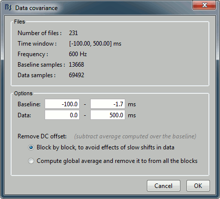
Repeat the same steps for run#02.
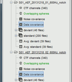
On the hard drive
Right-click on any noise covariance file > File > View file contents:
Structure of the noise/data covariance files: noisecov_*.mat / ndatacov_*.mat
Comment: String displayed in the database explorer to represent this file.
NoiseCov: [nChannels x nChannels] noise covariance: F * F' ./ (nSamples-1)
Unknown values are set to zero.FourthMoment: [nChannels x nChannels] fourth order moments: F.^2 * F'.^2 ./ (nSamples-1)
nSamples: [nChannels x nChannels] number of time samples that were used for each pair of sensors. This is not necessarily the same value everywhere, some channels can be declared as bad only for a few trials.
Related functions
process_noisecov.m: Function for process "Sources > Compute covariance (noise or data)"
bst_noisecov.m: Computes the data/noise covariance matrices.
panel_noisecov.m: Options panel.
Additional documentation
Forum: EEG reference: http://neuroimage.usc.edu/forums/showthread.php?1525#post6718
Forum: Data covariance and number of trials: https://neuroimage.usc.edu/forums/t/34094
Tutorial 22: Source estimation
Authors: Francois Tadel, Elizabeth Bock, Rey R Ramirez, John C Mosher, Richard M Leahy, Sylvain Baillet
This section describes how to estimate brain activity accounting for scalp recordings.
Contents
- Background
- Source estimation options
- Computing sources for an average
- Display: Cortex surface
- Recommended post-processing steps
- Display: MRI Viewer
- Display: MRI 3D
- Sign of constrained maps
- Unconstrained orientations
- Standardization of source maps
- Delete your experiments
- Computing sources for single trials
- Averaging in source space
- Note for beginners
- Averaging normalized values
- Display: Contact sheets and movies
- Model evaluation
- Advanced options: Minimum norm
- Advanced options: LCMV beamformer
- Advanced options: Dipole modeling
- Combining MEG+EEG for source estimation
- On the hard drive
- Additional documentation
Background
Estimating brain activity at potentially thousands of brain locations (determined by the forward head model) from much fewer sensor locations is a so-called ill-posed inverse problem. One implication is that an infinite number of source activity patterns may explain equivalently well the sensor data. These aspects are explained in detail here and here.
Such ill-posedness is not specific to EEG/MEG. It is quite typical in many other fields of science and engineering.
There is a vast EEG/MEG literature on the question. Brainstorm features three well-documented types of approaches: minimum-norm imaging, beamforming, and dipole modeling.
One common advantage between these approaches is that they are computationally efficient, even on large datasets. The estimates of brain source activity are derived via a linear recombination of sensor recordings. Brainstorm therefore computes a kernel ("a large matrix") conveniently stored in the database and that can be multiplied with sensor data arrays to obtain source time series, at specific brain locations, or across the entire brain.
Below we first describe the options of the minimum-norm imaging approach, then beamformers and dipole modeling. These latter are technically similar.
Source estimation options
Method
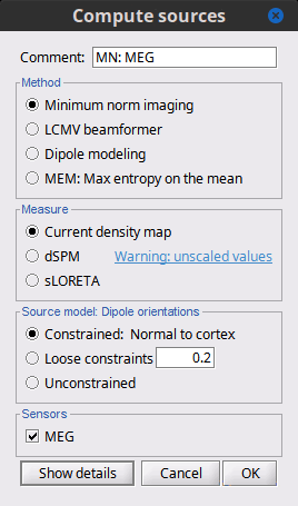
Minimum-norm (MN) imaging
- MN imaging estimates the amplitude of brain sources distributed across the brain or constrained to the cortex. The MN solution to the ill-posed EEG/MEG inverse problem is the one that best fits the sensor data with minimum overall amplitude of brain activity.
MN imaging requires the specification of noise statistics via a so-called noise covariance matrix. MEG users can best estimate noise statistics from an empty-room recording. If not available, as in EEG, noise covariance can be derived directly from recordings (e.g., from pre-stim segments, if relevant to the scientific question) or be assumed as uniform across sensors as described below.
Beamforming
- Brainstorm features the well-studied linearly constrained minimum variance (LCMV) beamformer to estimate source activity through a spatial filtering procedure. In lay terms, beamformer scans through all potential brain locations specified in the head model and estimates their respective contributions to sensor data, while attenuating the contributions from other brain regions.
Beamforming is technically similar to MN imaging, although it is more sensitive to approximations of the head model than MN imaging, and requires specific additional inputs. It is also blind to sources at different brain locations, but which time series are highly correlated.
LCMV beamformers require the specification of the data (noise+signal) covariance matrix, estimated directly from the recordings. LCMV source images can either be used as such, or post-processed, with a dipole model fitted at every time point of their largest peak(s). Please refer to the section further below for more detail about beamformers.
Dipole modeling
Brainstorm features a simple localization approach that adjusts the parameters of a single current dipole fitted to the sensor data at each point in time. As mentioned above, a LCMV-type map is first produced, and an equivalent current dipole is fitted at the strongest peak location of that map (more detail here).
Recommended option
- After exploring many, more sophisticated alternatives, our preference is to use simple and robust imaging approaches such as MN imaging or beamforming over single dipole scanning. However, this decision is often a matter of tradition in different resarch groups or subfields.
- Brainstorm enables the convenient comparison of these three approaches on your own data, with all possible sub-options, as detailed below.
MN imaging variants
By default, MN imaging estimates the amplitude of brain electrical currents at each grid location determined by the forward head model (i.e., either in volume or on the cortical surface). As discussed here, the currents are expressed in A-m. Brainstorm does not normalize by surface area (A/m, i.e., current surface density) or volume (A/m^2, i.e., current volume density). Nonetheless, we refer to this default setting as yielding a current density map.
Current density map option: implements a L2-minimum norm estimate of brain current. FOr consistency, Brainstorm's method is identical to MNE's. Please refer to the MNE manual (Section 6, "The current estimates") for a technical description. Units are scaled to pA-m.
To further compensate for the inhomogenous sensitivity of EEG/MEG with depth and orientation of the current flow, we recommend that the current density maps obtained with this option be further standardized using a z-score transformation with respect to a specific time segment of no interest (e.g., pre-stimulus baseline) or experimental condition (e.g., resting-state).
Alternatively, such standardization can be achieved directly with respect to global noise and data covariance statistics via the dSPM and sLORETA options.
dSPM [recommended]: the derivations are those of the dynamical Statistical Parametric Mapping approach by Dale et al. (2000), based on the default MN option above and scaled with respect to the noise covariance. The resulting dSPM maps are a set of z-scores. Units: unitless "z".
sLORETA: Standardized LOw Resolution brain Electromagnetic TomogrAphy approach proposed by Pasqual-Marqui (2002).. The default current density maps are normalized with respect to the theoretical data covariance, found as the sum of the noise covariance and a model of brain signal covariance (see original paper for detail). (Note that the sLORETA data covariance is not the empirical data covariance estimated directly from the data, as used in beamformers, but rather the theoretical “statistical” data covariance used in minimum norm estimation). Per Eq 16 and 17 of Pascual-Marqui’s technical details paper, Brainstorm employs sLORETA’s concept of the unitless Resolution Kernell R. Thus the units of Brainstorm’s sLORETA implementation are output in units of A-m, which are the units of the minimum norm source estimation, which pass through the square root of the inverted resolution kernel.
Source model: Dipole orientations [TODO]
The current flow of neural activity at each source localtion is modeled by the orientation of an equivalent current dipole. Brainstorm features the following options to determine this orientation:
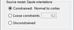
Constrained: Normal to cortex: this option is available only when working with "surface" grid locations (such as the cortical surface). Current dipoles are oriented normally to the cortical surface, to model the orientation of macrocolumns of pyramidal neurons perpendicular to the cortex.
Size of the imaging kernel: [Nvertices x Nchannels].Loose: This option is available only when working with "surface" grid locations (such as the cortical surface). In addition to a dipole normal to cortex as above, two additional dipoles are adeed in the tangential plane at each cortical location. Their amplitude is constrained below a fraction of the main normal dipole's. The recommended values are between 0.1 and 0.6. This option relaxes the constraint of strict orientation to the cortex to account for anatomical and physiological uncertainties.
Size of the imaging kernel: [3*Nvertices x Nchannels].Unconstrained: This option is available for both "surface" and "volume" source grids. There are 3 orthogonal dipoles at each grid location along the x, y, and z ("Cartesian") directions of the coordinate system.
Size of the imaging kernel: [3*Nvertices x Nchannels].Recommended option: The fully constrained option require only one dipole per source grid location, instead of three. Therefore, the source and kernel files are smaller, faster to compute and display. However, when using MRI templates instead of individual anatomy, loose/unconstrained orientation models may account for some of the model uncertainties (see this section).
Sensors

Brainstorm automatically detects the type of sensors (mEg, EEG, etc.) available from the head model selected for source imaging. In the example above, only MEG sensors are available. Select one or all the sensor types available you are interested in.
However, cross-modality calculations -- the fusion between MEG and EEG data to yield a joint source map -- are very sensitive to covariance calculations and head model approximations. As of Spring of 2018, we have also elected to NOT account for cross-covariances between different sensor types. If you wish to obtain a joint, multimodal source model, we recommend that you compute each source map separately and then combine them visually or quantitatively.
Computing sources for an average
We describe here a basic example of how to use Brainstorm to obtain a MN imaging maps of event-related average sensor data.
In Run#01, right-click on the average response for the deviant stim > Compute sources [2018].
Select the options: Minimum norm imaging, Current density map, Constrained: Normal to cortex.
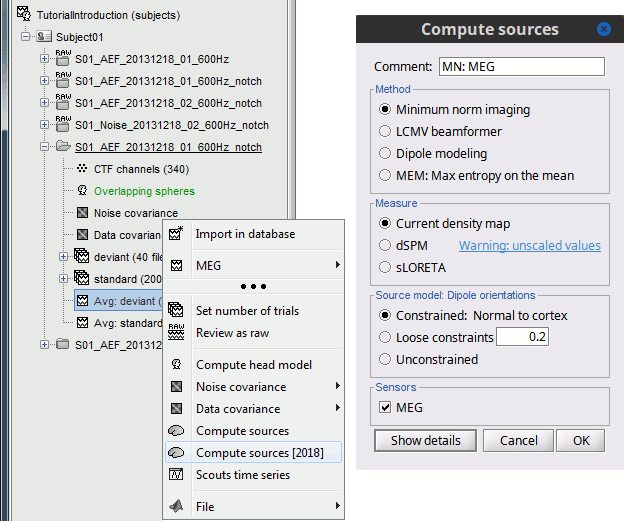
(The other "Compute sources" menu is for legacy options and implementations of the same imaging options.)The outcome of this process is a new dependent file of the sensor data, indicated with a brain icon. The file label (aka "comment") indicates "MN", which stands for "minimum-norm", and "Constr", which stands for "Constrained: normal orientation".
Display: Cortex surface
Right-click on this new source file with the brain icon and select > Cortical activations > Display on cortex.
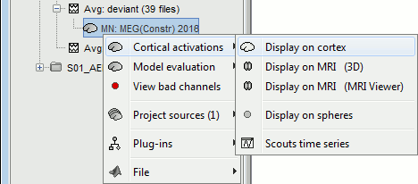
Double-click on the recordings for the deviant average to display the sensor time series alongside their brain source maps.
In the filter tab, add a low-pass filter at 40Hz to smooth the time series a bit.
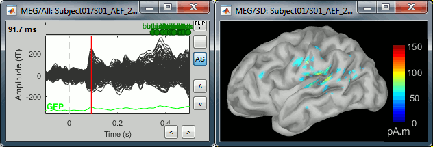
- Note how the display of the sensor and brain map windows are sync'd in time (click anywhere in the white portion of the time series window or use the left/right keyboard arrows to change the time stamp). You can also use all the menus and shortcuts introduced in the anatomy tutorial to use pre-set displays (0-6 keys).
Edit the display properties of the brain map in the Surface tab:
Amplitude: applies a minimum threshold to the source amplitude values displayed. The threshold is defined as a percentage ratio of the maximum amplitude value of the currrent color scale.
Min size: removes the smaller clusters in the source map, which number of source is smaller than the "min size" value entered.
Transparency: changes the opacity of the source map on the cortex surface.
Note that these parameters only adjust the visualization of source maps. They do not have effect on the actual source time series.
A few more words about the amplitude threshold parameter:
The maximum of the current colorbar depends on the Sources colormap parameters. If "Maximum: Global" is selected, the maximum indicated should be around 150 pA.m in the present dataset. This value represents the maximum of the source map across the entire dataset (across space and time). You can change the colorbar maximum value with the colormap option "Maximum: Custom".
On the screen capture below, the threshold value is set to 20%: only sources with amplitudes greater than 0.20*150 = 30 pA.m are shown.
The threshold value is shown in the colorbar with a horizontal white line.In the current data example, the source map should indicate strong activations around the primary auditory cortex around 91ms, bilaterally.
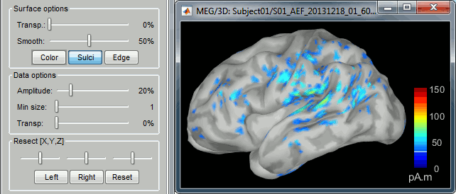
Recommended post-processing steps
The original source maps may look noisy or patchy. This is due to the strict orientation constraint used in the brain mapping procedure, which emphasizes the sensitivity of brain current strengths to the curvature of the cortex (this effect is more pronounced with MEG than EEG).
Please be cautious not to interpret disconnected colored patches as distinct brain activations without further post processing. The absolute spatial resolution of MEG source mapping is limited (~5-10mm, worse in EEG), although its relative resolution between experimental conditions, hence with post processing, can be much finer (1mm or less, see for instance this retinotopy study).
For now, you may generate smoother versions of the source maps by applying a spatial smoothing process (process "Sources > Spatial smoothing"), or using unconstrained source models, or standardizing source amplitude by applying a z-score transformation with respect to a time period of reference.
Brain maps obtained with dSPM or sLORETA are also standardize, more immune to orientation confounds (see below for more detail).
Display: MRI Viewer
Right-click on the source file for the deviant average > Cortical activations > Display on MRI (MRI Viewer).
See Brainstorm's MRI Viewer detailed tutorial in Sections #2 and #3.
This display shows cortical source activity interpolated in the the MRI volume. Set the amplitude threshold to 0% to visualize the cortex ribbon used onto which source activity is mapped.
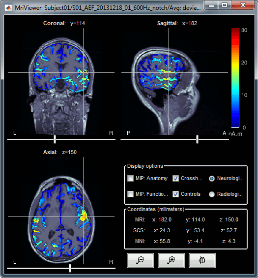
- Visualization parameters:
MIP Anatomy: check this box to obtain a "glass brain" view of the structural MRI, across all three spatial dimensions. MIP stands for "Maximum Intensity Projection"
MIP Functional: to obtain a glass brain view of the source map.
Amplitude threshold: in the Surface tab of the main Brainstorm window, to apply a threshold on the source map, as explained for the 3-D cortex view above.
Current time: shows the current time stamp in the data recordings, at the top-right of the main Brainstorm window. You also use the right/left arrows to move in time, or click anywhere in the white area of the sensor time series window.
Overlay options: Right-on the figure to get access additional options.
Smooth: Increase this value to smooth the source map further, for visualization purposes. This parameter defines the size of the smoothing kernel, in number of voxels.
Interpolation sources>MRI: Parameters to compute the interpolation on the MRI volume of the source maps, available on a source space of 15000 points located on the cortex surface. This procedure associates to each of the millions of MRI voxels a value computed from these 15000 source values. This menu lets you control some parameters of this interpolation.
Interpolate values: If enabled, performs a distance-weighted interpolation with 3 nearest neighbors (default for source results). If disable, performs a single nearest-neighbor lookup instead (useful to represent integer values that should not be interpolated, such as parcel labels).
Distance threshold: Maximum distance between a colored voxel and a grid point.
Resolution: Spatial resolution of the interpolated source maps. By default, the interpolation computes a source volume downsampled by a factor 3 with respect to the anatomical MRI, in order to make the computation faster. In that case, each colored element has a dimension of 3x3x3 voxels. If a higher resolution is needed (e.g. for displaying SEEG data) this parameter can be lowered to 1 or 2 voxels. Using a 1-voxel resolution requires the computation of 3*3*3=27 times more voxel values than with the default option, leading to much longer computation times.
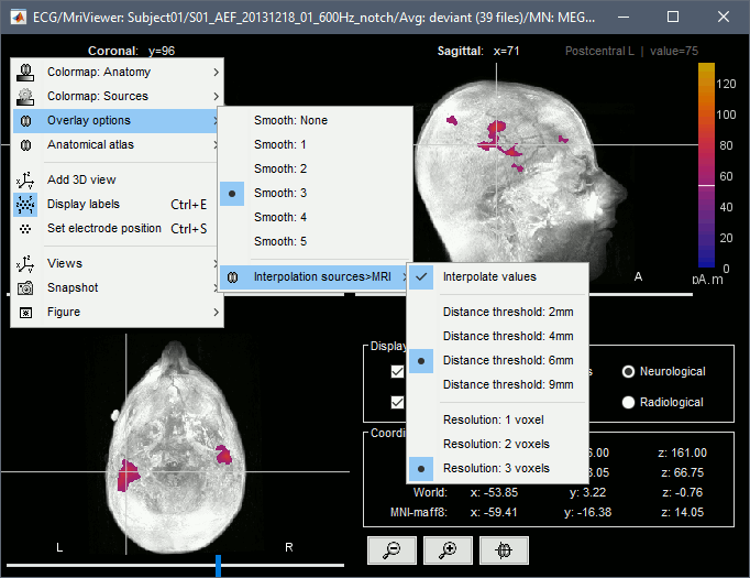
Display: MRI 3D
Right-click on the source file for the deviant average > Cortical activations > Display on MRI (3D).
We detailed this feature in the previous tutorial sections about MRI and surface visualization.
Keep right mouse button pressed and move the mouse to change the MR slices displayed. You can also use the Resect panel of the Surface tab.
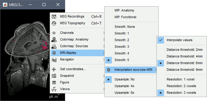
Sign of constrained maps
Source brain maps consist of time series that are complex curves of positive and negative values.
You can visualize how the sign of source amplitudes is distributed across the cortex using the cortical display of sources: set the amplitude threshold to 0%, then make sure the colormap shows relative (i.e., both positive and negative) values. For this, right click over the colorbar Colormap: Sources > uncheck the "Absolute values" option. At any time, you can double-click on the colorbar to reset the colormap options to default values.
As shown below, a typical brain map will show stripes of positive and negative values, with sign changes around sulcal locations. This is another manifestation of the limited absolute spatial resolution of MEG/EEG source mapping. Sources of opposite sides of sulcus are oriented in opposite directions by default. Source mapping shows they have oppositive signs meaning that the respective neural currents are estimated as flowing in the same direction. We will see later how this sign ambiguity can be managed via either the processing of rectified source time series (if you wish to map source amplitude effects only). It is crucial to preserve the sign though if you are in interested in frequency specific brain activity, such as spectral, time-frequency and connectivity analyses.
More on sign ambiguity: On opposite walls of a sulcus, brain source are very close to each other, with opposite orientations. If the true brain activity sits only on one side of a sulcus as shown below with a green arrow, the MN-imaging brain map lower spatial resolution will spread the estimated currents over multiple nearby locations, shown with the red and blue arrows below, which have opposite default directions that are imposed by anatomy (dipoles pointing outwards the cortical surface). The signs of the current flows will be opposite, with positive values (red arrows) on one side of the sulcus and negative values on the other side (blue arrows).
For visualization purposes, we are mostly interested at this stage in visualizing the magnitude of brain activity, hence the default colormap option "absolute values" being selected.
Unconstrained orientations
The "loose constraints" and "unconstrained" options for source orientations yield 3 time series per brain location (from three orthogonal elementary sources), which increases the dimensionality of the source maps, hence complexify their interpretation, but produces smoother renderings of current flows. We recommend these options when using an MRI template instead of the individual MRI volume of study participants, or when studying subcortical brain structures. Unconstrained maps can subsequently be converted to "flat" maps, i.e. a single orientation per location, which may be needed for some processes.
Here we will illustrate the fully unconstrained case. The procedure for the loose constraints options is similar.
In Run#01, right-click on the trial average of the deviant condition > Compute sources [2018].
Select the options: Minimum norm imaging, Current density map, Unconstrained.Double-click on the source file produced (brain icon, labelled with "Unconstr") and on the corresponding sensor data file. The two brain maps below represent the same file at 91ms, with different colormap options (absolute values on the left, relative values on the right). Explanations below.
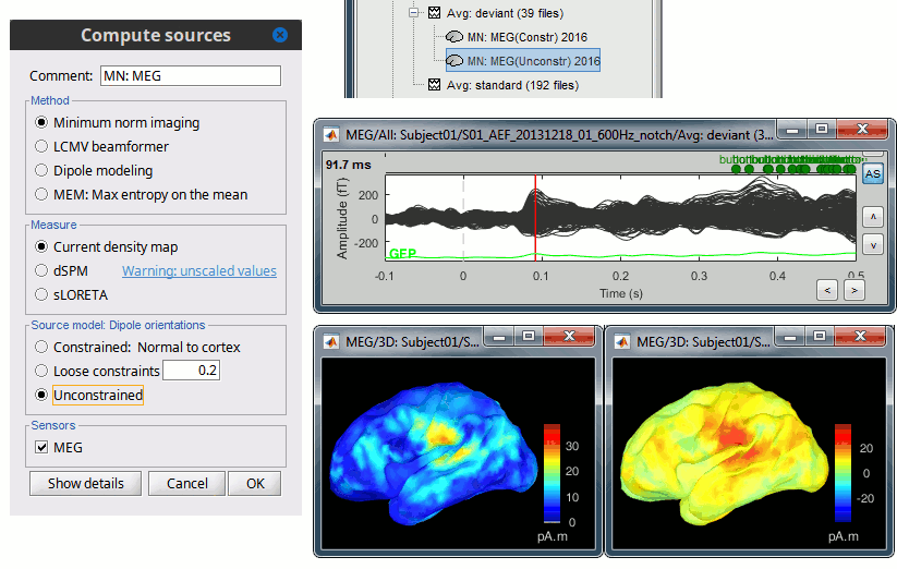
Again, using unconstrained/loose source orientations consists of triplets of dipoles with orthogonal orientations at each cortex location. To display their activity in a visually-meaningful manner, we first need to reduce the dimensions of the source data and color code the outcome. Brainstorm displays the norm of the vectorial sum of the three orientations at each vertex.
S = sqrt(Sx2 + Sy2 + Sz2)

This explains that only positive values are displayed over the source map. Note that the actual full values along each orientation (x,y,z) are signed and can be retrieved from the source file for further derivations (e.g., spectral analyses).
- The unconstrained/loose orientation maps are typically smoother than with the constrained orientation option (but see post-processing steps below) because they are less overly sensitive to changes in the curvature of the cortex.
You may delete the unconstrained source file: we will not use this option further in the introduction tutorials. Please refer to the tutorial EEG and epilepsy for further exploration of this option.
Standardization of source maps
Standardization procedures can compensate some of the bias of MN imaging source maps towards superficial source locations (in both MEG and EEG) and radially oriented current flows (in MEG). It also enables a fairer comparison of brain activity between individuals, based on its relative change with a data segment of reference.
Reference data segments can be extracted from empty-room recordings (MEG), pre-stimulus baseline or resting state data (MEG and EEG).
dSPM and sLORETA proceed to such standardization within their respective source mapping procedures. Brainstorm also features a Z-score normalization process, which enables a versatile definition of the reference data segment.
Source map standardization does not alter the dynamics of the source time series and only scales their respective amplitude changes. The scaling factors are different at each brain location, hence the resulting source maps will look different than the original MN images, but with the same temporal dynamics.
dSPM, sLORETA (embedded standardization)
In Run#01, right-click on the average sensor data of the deviant condition > Compute sources [2018].
Select successively the two normalization options: dSPM, sLORETA, (constrained).

Double-click on all the resulting source files to compare them (screen capture below is at the 143-ms time point):

Current density maps (MN imaging): without further standardization, MN imaging tends be biased towards the most superficial gyral crowns (see Z-score procedure below).
dSPM: compensates some of this bias. The amplitude of brain maps are converted to z-scores. You may adjust the z-scores with the number of trials used to obtain the sample average via specific process "Sources > Scale averaged dSPM" (see Averaging normalized values).
sLORETA: the statistics are proper to the method and therefore, are not related to z-scores.
Z-score transformation of brain maps
The Z-transformation of MN imaging brain maps centre source amplitudes around their mean over a reference segment, and scale them with respect to their standard deviation over the same reference segment: Z = (Data - μ) / σ
- The mean and standard deviation parameters are estimated from the data and are specific of each source location. Hence, sources with lower fluctuations over the reference segment (e.g., with less noise, or overall smaller amplitude) will be boosted by the transformation.
In Process1: Select the constrained current density map (file MN: MEG(Constr)).
Run process "Standardize > Baseline normalization", [-100,-1.7]ms, Z-score transformation
Do not select "Use absolute values" as for now, we wish to preserve the sign of source amplitudes.
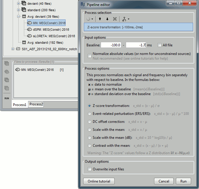
Double-click on the new brain map file (with the "| zscore" tag).

- We can appreciate that the standardized map is now qualitatively similar to dSPM and sLORETA versions.
- A map value of 3 means that the source amplitude at this time point is 3 times above the typical amplitude of that same source during the reference segment.
Please note Brainstorm's online filters do not affect the z-transformed source maps. Using the Filter tab and applying a bandpass filter will update the display all sensor time series and source maps on display, except the z-transormed maps.
If you wish to use a reference segment from another data file (e.g., a resting state recording as reference for the current task recording), use the Process2 process tab by dragging and dropping the reference source map in the Files A list on the left, and the source maps to be standardized in the Files B list on the right.
Recommended options
Use non-standardized current density maps (MN imaging) for:
- Computing imaging kernels shared across single trials.
- Averaging files across several MEG/EEG runs.
- Deriving spectral, time-frequency decompositions, phase-amplitude, or connectivity measures on single trials.
Use standardized maps (dSPM, sLORETA, Z-score) for:
- Producing source maps of trial averages (ERP/ERF).
- Before running a group analysis of source maps.
- Recommended standardization approach:
- dSPM and sLORETA are convenient linear measures which are easy to manipulate with Brainstorm.
- sLORETA maps are spatially smoother but with no direct statistical interpretation without further inference testing.
- dSPM and Z-score maps are statistically interpretable as excursions with respect to a reference data segment (Z-score), or with respect to noise covariance statistics (dSPM).
Delete your experiments
Before we proceed with the rest of the tutorial, please delete the source maps computed so far.
Select all the source files you computed until now and delete them.
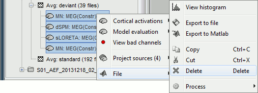
Computing sources for single trials
MN imaging models are linear: their respective imaging kernels can be pre-computed from anatomy and sensor locations only, then can be applied at once on long, ongoing or several epoched data segments on the fly. Here we show how to obtain source maps across multiple single trial epochs.
Right-click on the head model or the folder for Run#01 > Compute sources [2018].
Select: Minimum norm imaging, Current density map, Constrained: Normal to cortex
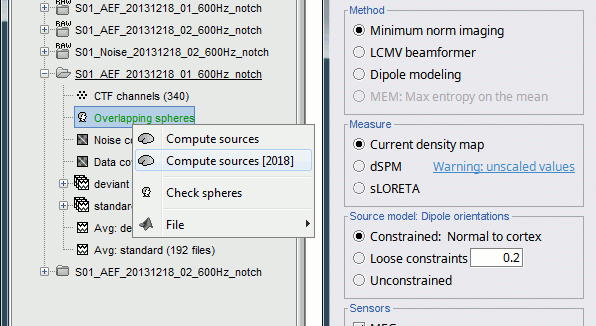
This procedure produces a shared imaging kernel (white brain icon) that is comon to all data files in Run #01. If you right-click on this new file, a warning message pops up that says "Inversion kernel". This file does not contain source maps, only the linear operator (kernel) to convert the sensor data into source maps.
All data files in Run #01 (averages and single epochs) now show a link to a source file (grey brain icon), which is a virtual brain map that is computed on the fly when visualized: Brainstorm multiplies the imaging kernel by the sensor data time series, for greater computational and data storage efficacy. You may now visualize and manipulate these virtual source maps just like the maps we computed above.
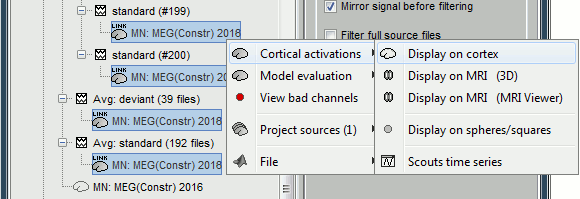
Averaging in source space
Computing the average
First compute the same source model for the the second acquisition run.
In Run#02, right-click on the head model or the folder > Compute sources [2018].
Select: Minimum norm imaging, Current density map, Constrained: Normal to cortex
Now we have the source maps available for all the recordings, we can average them in source space across runs. This allows us to average MEG recordings that were recorded with different head positions (in this case Run#01 and Run#02 have different channel files so they could potentially have different head positions preventing the direct averaging at the sensor level).
Thanks to the linearity of the minimum norm model: MN(Average(trials)) = Average(MN(trials))
The two following approaches are equivalent:- Averaging the sources of all the individual trials across runs,
- Averaging the sources for the sensor averages that we already computed for each run.
- We will use the second option: using the sources for the sensor-level averages. It is a lot faster because it needs to read 4 files (one average file per run and per condition) instead of 456 files (total number of good trials in the two runs).
Drag and drop to the Process1 tab the average recordings for Run01 and Run02, then press the [Process sources] button on the left to select the source files instead of the MEG recordings.
Run process "Average > Average files":
Select "By trial group (subject average)" to average together files with similar names.
Select "Arithmetic average" function.
Check "Weighted average" to account for the different numbers of trials in both runs.
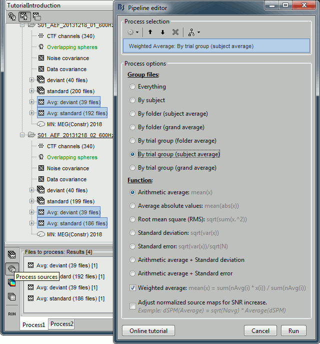
The two averages that are produced (one for each condition) are saved in the folder Intra-subject. This is where all the files computed using information from multiple folders within the same subject are saved. If you prefer to have them somewhere else, you can create new folders and move them there, just like you would do with a regular file explorer.
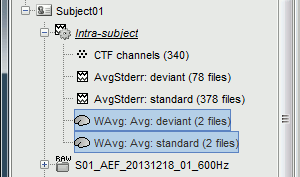
The file comments say "2 files" because they were computed from two averages each (one from each run), but the number of corresponding trials is correctly updated in the file structure.
Right-click on each of them > File > View file contents, and check the Leff field:
78 trials for the deviant condition, 378 trials for the standard condition.Double-click on the source averages to display them (deviant=top, standard=bottom).
Open the sensor-level averages as a time reference.
Use the predefined view "Left, Right" for looking at the two sides at the same time (shortcut: "7").
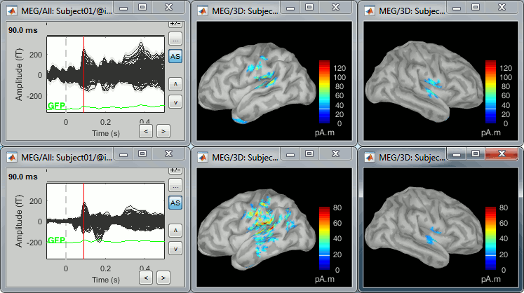
Visualization filters
Note that opening the source maps can be very long because of the filters for visualization. Check in the Filter tab, you may have a filter applied with the option "Filter all results" selected. In the case of averaged source maps, the 15,000 source signals are filtered on the fly when you load a source file. This filtering of the full source files can take a significant amount of time, consider unchecking this option if the display is too slow on your computer.
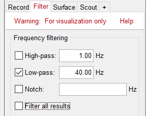
- It was not a problem until now because the source files were saved in the compact form (Kernel*recordings) and the visualization filters were applied on the recordings, then projected to the source space. This fast option is not available anymore with these averages across runs.
- The visualization filters will not be available anymore after we apply a Z-score normalization. If we want to display Z-score source maps that are smoothed in time, we will have to apply explicitly the filters on the file, with the Process1 tab.
Low-pass filter
- Clear the Process1 list, then drag and drop the new averages in it.
Run process "Pre-process > Band-pass filter": [0,40] Hz
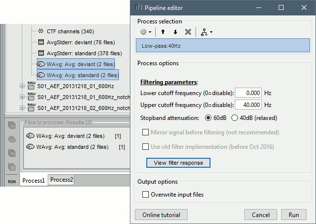
Epochs are too short: Look at the filter response, the expected transient duration is at least 78ms. The first and last 78ms of the average should be discarded after filtering. However, doing this would get rid of almost all the 100ms baseline, which we need for normalization. As mentioned here, we should have been importing longer epochs in order to filter and normalize the averages properly.
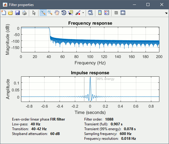
Z-score normalization
- In Process1, select the two filtered averages.
Run process "Standardize > Baseline normalization", baseline=[-100,-1.7]ms, Z-score.
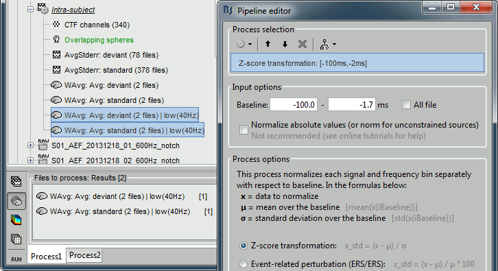
Four new files are accessible in the database: two filtered and two filtered+normalized.
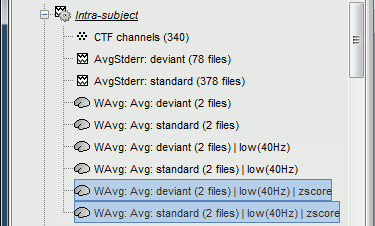
Double-click on the source averages to display them (deviant=top, standard=bottom).
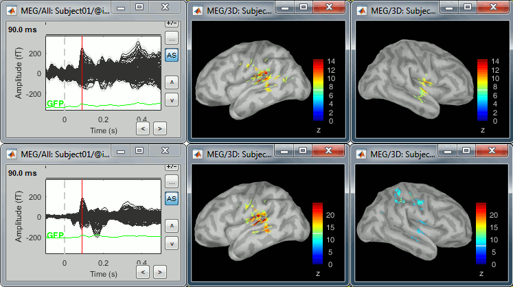
- The Z-score source values at 90ms are higher for the standard condition (~25) than for the deviant condition (~15). We observe this because the two conditions have very different signal-to-noise ratios. The standard condition has about 5x more trials, therefore the standard deviation over the baseline is a lot lower, leading to higher Z-score.
Delete the non-normalized filtered files, we will not use them in the following tutorials.
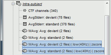
Note for beginners
Everything below is advanced documentation, you can skip it for now.
Averaging normalized values
Averaging normalized source maps within a single subject requires more attention than averaging current density maps. Since averaging reduces variance, the resulting source maps will have a different statistical distribution than the nominal distribution of the individual maps.
For example, averaging z-score normalized maps will result in maps with variance less than 1. The same holds true for dSPM maps. Assuming independent samples, the variance of an average of N maps drops by 1/N. For this reason, it is generally recommended to select the "Weighted average" option in the ‘Average files’ process when averaging trials or source maps (which performs mean(x) = (N1*sum(x1(i)) + N2*sum(x2(i)) + …)/ (N1+N2+…) ) in order to keep track of the number of samples and the actual variance of averaged statistical maps.
dSPM
- An averaged dSPM map has variance equal to 1/N (and thus standard deviation equal to 1/sqrt(N)). Therefore one could multiply the averaged dSPM map by sqrt(N) in order to maintain variance 1 under the null hypothesis. In previous versions of Brainstorm, this was done automatically when visualizing the files, and when averaging source maps with the option "Adjust normalized source maps for SNR increase". To simplify the interface and make the interpretation of maps more intuitive and consistent with other cases (min-norm, z-scored), we now dropped this option. Thus averaging dSPM maps now results in maps with variance less than 1, and is consistent with handling min-norm, z-scored and sLORETA maps.
Ajusting an averaged dSPM file by this sqrt(N) factor is still possible manually, eg. in order to visualize cortical maps that can be interpreted as Z values. Select the average dSPM files in Process1 and run process "Sources > Scale averaged dSPM". This should be used only for visualization and interpretation, scaled dSPM should never be averaged or used for any other statistical analysis.
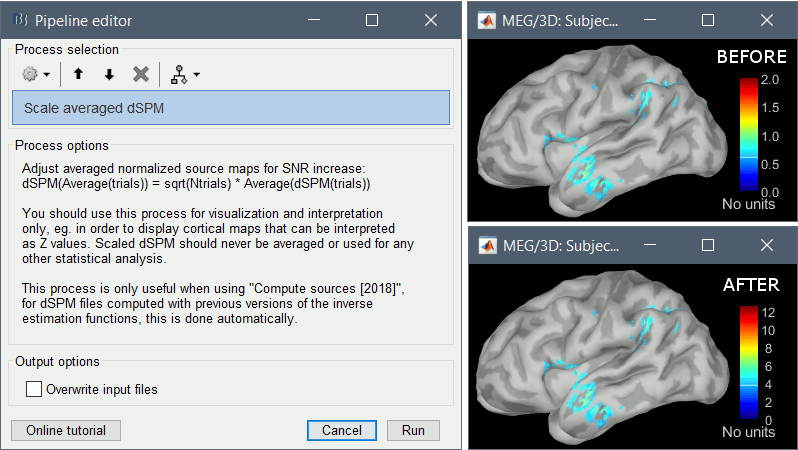
Z-score
- The same SNR issues arise while averaging Z-scores: the average of the Z-scores is lower than the Z-score of the average.
When computing averages at the subject level: Always avoid averaging Z-score maps.
Average the current density maps, then normalize.
sLORETA
- This normalization is not based on the SNR of signal, but rather on the spatial smoothness of the maps. Managing these maps is similar to min-norm maps: the variance of the individual maps is not explicitly modeled or known analytically.
- As in other cases, sLORETA(Average(trials)) = Average(sLORETA(trials)), and this relationship is guaranteed to hold with averaging uneven number of samples when using the option "Weighted average".
Display: Contact sheets and movies
A good way to represent what is happening in time is to generate contact sheets or videos. Right-click on any figure and go to the menu Snapshot to check out all the possible options. For a nicer result, take some time to adjust the size of the figure, the amplitude threshold and the colormap options (hiding the colorbar can be a good option for contact sheets).
A time stamp is added to the captured figure. The size of the text font is fixed, so if you want it to be readable in the contact sheet, you should make you figure very small before starting the capture. The screen captures below where produced with the colormap "hot".
Contact sheet: Right-click on any figure > Snapshot > Time contact sheet: Figure
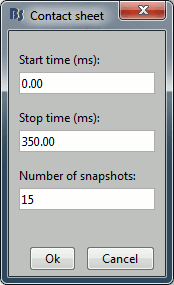
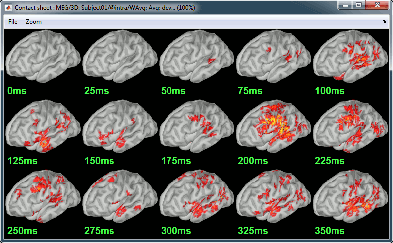
Movies: Right-click on any figure > Snapshot > Movie (time): All figures
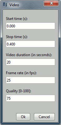
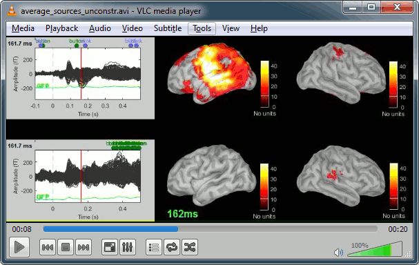
Model evaluation
One way to evaluate the accuracy of the source reconstruction if to simulate recordings using the estimated source maps. This is done simply by multiplying the source time series with the forward model:
MEG_simulated [Nmeg x Ntime] = Forward_model [Nmeg x Nsources] * MN_sources [Nsources x Ntime]
Then you can compare visually the original MEG recordings with the simulated ones. More formally, you can compute an error measure from the residuals (recordings - simulated).
To simulate MEG recordings from a minimum norm source model, right-click on the source file, then select the menu "Model evaluation > Simulate recordings".
Open side-by-side the original and simulated MEG recordings for the same condition:
Advanced options: Minimum norm
Right-click on the deviant average for Run#01 > Compute sources [2018].
Click on the button [Show details] to bring up all the advanced minimum norm options.
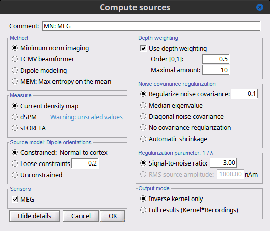
Depth weighting
Briefly, the use of various depth weightings was far more debated in the 1990s, before the introduction of MNE normalization via dSPM, sLORETA, and other "z-scoring" methods, which mostly cancel the effects of depth weighting (put another way, after normalization min norm results tend to look quite similar whether depth weighting is used or not).
By modifying the source covariance model at each point in the source grid, deeper sources are "boosted" to increase their signal strength relative to the shallower dipoles; otherwise, the resulting MNE current density maps are too dominated by the shallower sources. If using dSPM or sLORETA, little difference in using depth weighting should be noted. To understand how to set these parameters, please refer to the MNE manual. (options --depth, --weightexp and --weightlimit).
Noise covariance regularization [TODO]
MNE and dipole modeling are best done with an accurate model of the noise covariance, which is generally computed from experimental data. As such, these estimates are themselves prone to errors that arise from relatively too few data points, weak sensors, and strange data dependencies that can cause the eigenspectrum of the covariance matrix to be illconditioned (i.e. a large eigenvalue spread or matrix condition number). In Brainstorm, we provide several means to "stabilize" or "regularize" the noise covariance matrix, so that source estimation calculations are more robust to small errors.
Regularize noise covariance: The L2 matrix norm is defined as the largest eigenvalue of its eigenspectrum. This option adds to the covariance matrix a diagonal matrix whos entries are a fraction of the matrix norm. The default is 0.1, such that covariance matrix is stabilized by adding to it an identity matrix that is scaled to 10% of the largest eigenvalue.
Median eigenvalue: The eigenspectrum of MEG data can often span many decades, due to highly colored spatial noise, but this broad spectrum is generally confined to the first several modes only. Thus the L2 norm is many times greater than the majority of the eigenvalues, and it is difficult to prescribe a conventional regularization parameter. Instability in the inverse is dominated by defects found in the smallest eigenvalues. This approach stabilizes the eigenspectrum by replicating the median (middle) eigenvalue for the remainder of the small eigenvalues.
Diagonal noise covariance: Deficiencies in the eigenspectrum often arise from numerical inter-dependencies found among the channels, particularly in covariance matrices computed from relatively short sequences of data. One common method of stabilization is to simply take the diagonal of the covariance matrix and zero-out the cross-covariances. Each channel is therefore modeled as independent of the other channels. The eigenspectrum is now simply the (sorted) diagonal values.
No covariance regularization: We simply use the noise covariance matrix as computed or provided by the user.
Automatic shrinkage: Stabilization method of Ledoit and Wolf (2004), still under testing in the Brainstorm environment. Basically tries to estimate a good tradeoff between no regularization and diagonal regularization, using a "shrinkage" factor. See Brainstorm code "bst_inverse_linear_2018.m" for notes and details.
Recommended option: This author (Mosher) votes for the median eigenvalue as being generally effective. The other options are useful for comparing with other software packages that generally employ similar regularization methods. [TODO]
Regularization parameter [TODO]
In minimum norm estimates, as mentioned above in the comparisons among methods, the data covariance matrix is essentially synthesized by adding the noise covariance matrix to a modeled signal covariance matrix. The signal covariance matrix is generated by passing the source prior through the forward model. The source prior is in turn prescribed by the source model orientation and the depth weighting.
A final regularization parameter, however, determines how much weight the signal model should be given relative to the noise model, i.e. the "signal to noise ratio" (SNR). In Brainstorm, we follow the definition of SNR as first defined in the original MNE software of Hamalainen. The signal covariance matrix is "whitened" by the noise covariance matrix, such that the whitened eigenspectrum has elements in terms of SNR (power). We find the mean of this spectrum, then take the square root to yield the average SNR (amplitude). The default in MNE and in Brainstorm is "3", i.e. the average SNR (power) is 9.
Signal-to-noise ratio: Use SNR of 3 as the classic recommendation, as discussed above.
RMS source amplitude: An alternative definition of SNR, but still under test and may be dropped. [TODO]
Output mode
As mentioned above, these methods create a convenient linear imaging kernel that is "tall" in the number of elemental dipoles (one or three per grid point) and "wide" only in the number of sensors. At subsequent visualization time, we efficiently multiply the kernel with the data matrix to compute the min norm images.
For some custom purposes, however, a user may find it convenient to pre-multiply the data matrix and generate the full source estimation matrix. This would only be recommended in small data sets, since the full results can become quite large.
Kernel only: Saves only the linear inverse operator, a model that converts sensor values into source values. The size of this matrix is: number of sources (15000) x number of MEG sensors (274). The multiplication with the recordings is done on the fly by Brainstorm in a transparent way. For long recordings or numerous epochs, this form of compact storage helps saving a lot of disk space and computation time, and it speeds up significantly the display. Always select this option when possible.
Full results: Saves in one big matrix the values of all the sources (15,000) for all the time samples (361). The size in memory of such a matrix is about 45Mb for 600ms of recordings. This is still reasonable, so you may use this option in this case. But if you need to process longer recordings, you may face "Out of memory" errors in Matlab, or fill your hard drive quickly.
- Full results [15000x361] = Inverse kernel [15000x274] * Recordings [274x361]
Advanced options: LCMV beamformer
As mentioned in the introduction above, two other methods can be selected for source estimation, a beamformer and dipole modeling. In this section, we review the options for the beamformer. On top of the noise covariance matrix, you need to estimate a data covariance matrix in order to enable the option "LCMV beamformer" in the interface.
Note that pre-whitening with the noise covariance matrix has not yet been implemented for the LCMV beamformer, and only the data covariance is used in the current version. The noise covariance has no impact on the LCMV beamformer results. However, if there is no noise covariance file available in the database, the "Compute sources" interface returns an error: to go around this limitation, you may select the "No noise modeling (identity matrix)" option in the contextual menu for the noise covariance.
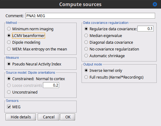
Measure
The only option "Pseudo Neural Activity Index" (PNAI), is named after the definition of the Neural Activity Index (NAI). We have modified Van Veen’s definition to rely strictly on the data covariance, without need for a separate noise covariance matrix, but the basic premise is the same as in dSPM, sLORETA, and other normalizations. Viewing the resulting "map," in an identical manner to that with MNE, dSPM, and sLORETA described above, reveals possibly multiple sources as peaks in the map. Note that PNAI scores are unitless, because they correspond to standardized statistical fluctuations of neural currents. In this way, PNAI scores are analogous to z-scoring.
Dipole orientations
We recommend you choose "unconstrained" and let the later Dipole scanning process, which finds the best fitting dipole at each time point, optimize the orientation with respect to the data.
Data covariance regularization
Same definitions as in MNE, only applied to the data covariance matrix, rather than the noise covariance matrix. Our recommendation is to use median eigenvalue.
Advanced options: Dipole modeling
Dipole modeling fits a single dipole at each potential source location to produce a dipole scanning map. This map can be viewed as a indication of how well, and where, the dipole fits at each time point. However, we recommend using the subsequent best-dipole fitting routine (dipole scanning) to determine the final location and orientation of the dipole (one per time point). Please note that this function does not fit multiple simultaneous dipoles.
Although not widely recognized, dipole modeling and beamforming are more alike than they are different – when comparing the inverse operators required to compute the dipole scanning map (dipole modeling) and the beamformer output map (LCMV), we see that they differ only in that the former uses an inverse noise covariance matrix while the latter replaces this with the inverse of the data covariance.
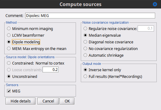
Measure
This field is now missing, but the resulting imaging kernel file is directly analogous to the PNAI result from LCMV beamforming. The user can display this scanning measure just as with the LCMV case, where again the normalization and units are a form of z-scoring.
Dipole orientations
Use "unconstrained source" modeling and let the process "dipole scanning" optimize the orientation of the dipole for every time instance.
Noise covariance regularization
Similarly, use "median eigenvalue".
The tutorial "MEG current phantom (Elekta)" demonstrates dipole modeling of 32 individual dipoles under realistic experimental noise conditions.
Combining MEG+EEG for source estimation
Magnetoencephalography and EEG sensor data can be processed jointly to produce combined source estimates. Joint processing presents unique challenges because EEG and MEG use head models that exhibit differing sensitivities to modeling errors, which can in turn lead to inconsistencies between EEG and MEG with respect to the (common) source model. In practice joint processing is relatively rare (Baillet et al., 1999). However, these data are complementary, which means that joint processing can potentially yield insights that cannot be seen with either modality alone.
For example, in the evoked responses in the data set used here, the first peak over the occipital areas is observed in MEG (90 ms) slightly before EEG (110 ms). This delay is too large to be caused by acquisition imprecisions. This indicates that we are not capturing the same brain processes with the two modalities, possibly because the orientation and type of activity in the underlying cortical sources is different.
MEG and EEG have different sensitivities to source orientation and depth. Given the challenges of joint processing, our advice is to first look at the source reconstructions for the two modalities separately before trying to use any type of fusion technique.
On the hard drive
Constrained shared kernel
Right-click on a shared inverse file in the database explorer > File > View file contents.
Structure of the source files: results_*.mat
Mandatory fields:
ImagingKernel: Linear inverse operator that must be multiplied by the recordings in order to get the full source time series. If defined, ImageGridAmp must be empty.
- Size for constrained sources [Nsources x Nchannels]
- Size for unconstrained sources [3xNsources x Nchannels]. Order of sources: source1.x, source1.y, source1.z, ... sourceN.z)
ImageGridAmp: Full source time series, in Amper.meter. If this field is defined, ImagingKernel must be empty. If you want this field to be set instead of ImagingKernel, make sure you select the advanced option Full results when estimating the sources.
- Size for constrained sources [Nsources x Ntime]
- Size for unconstrained sources [3xNsources x Ntime]. Order of sources: source1.x, source1.y, source1.z, ... sourceN.z)
Time: [1 x Ntime] Time values for each sample recorded in F, in seconds.
nComponents: Number of dipoles per grid point: 1=Constrained, 3=Unconstrained, 0=Mixed. In the case of mixed head models, the atlas GridAtlas documents region by region how the list of grid points matches the list of dipoles.
Function: Type of values currently saved in the file: 'mn', 'mnp', 'dspm', 'dspm2018', 'dspm2018sc', 'sloreta', 'lcmv', 'lcmvp', 'lcmvnai', 'lcmvpow', 'gls', 'glsp', 'glsfit', 'glschi', 'zscore', 'ersd'...
HeadModelType: Type of source space used for this head model ('surface', 'volume', 'mixed').
HeadModelFile: Relative path to the head model used to compute the sources.
SurfaceFile: Relative path to the cortex surface file related with this head model.
Atlas: Used only by the process "Sources > Downsample to atlas".
GridLoc: [Nvertices x 3], (x,y,z) positions of the grid of source points. In the case of a surface head model, it is empty and you read directly the positions from the surface file.
GridOrient: [Nvertices x 3], direction of the normal to the surface for each vertex point (copy of the 'VertNormals' matrix of the cortex surface). Empty in the case of a volume head model or unconstrained sources.
GridAtlas: Atlas "Source model" used with mixed source models.
GoodChannel: [1 x Nchannels] Array of channel indices used to estimate the sources.
DataFile: Relative path to the recordings file for which the sources where computed. If this field is set, the source file appears as a dependent of the DataFile.
Comment: String displayed in the database explorer to represent this file.
History: Operations performed on the file since it was create (menu "View file history").
Optional fields:
Options: Structure that contains all the options of the inverse calculation. This is saved in the file only for bookkeeping.
Whitener: Noise covariance whitener computed in bst_inverse_linear_2018.m
DataWhitener: Data covariance whitener computed in bst_inverse_linear_2018.m
SourceDecompVa: [3 x Nsources] Concatenated right singular vectors from the SVD decomposition of the whitened leadfield for each source (only for unconstrained sources).
SourceDecompSa: [3 x Nvertices] Vector diagonal of the singular values from the SVD decomposition of the whitened leadfield for each source (only for unconstrained sources).
Std: For averaged files, number of trials that were used to compute this file.
DisplayUnits: String, force the display of this file using a specific type of units.
ChannelFlag: [Nchannels x 1] Copy of the ChannelFlag field from the original data file.
Leff: Effective number of averages. For averaged files, number of trials that were used to compute this file. For source files that are attached to a data file, we use the Leff field from the data file.
Full source maps
In Intra-subject, right-click on one of the normalized averages > File > View file contents.
This file has the same structure as a shared inverse kernel, with the following differences:
It contains the full time series (ImageGridAmp) instead of an inverse operator (ImagingKernel).
The Z-score process updated the field Function ('mn' => 'zscore')
Source links
- The links are not real files on the hard drive, if you select the menu "View file contents" for any of them it would display the structure of the corresponding shared kernel.
They are saved in the database as strings with a specific structure: "link|kernel_file|data_file". This string associates a shared inverse operator with some recordings. The two files have to be available to load the this file. All the functions in Brainstorm are equipped to reconstruct the full source matrix dynamically.
Filename tags
_KERNEL_: Indicates that the file contains only an inverse kernel, it needs to be associated with recordings to be opened.
Useful functions
in_bst_results(ResultsFile, LoadFull, FieldsList): Load a source file and optionally reconstruct the full source time series on the fly (ImagingKernel * recordings).
in_bst(FileName, TimeBounds, LoadFull): Load any Brainstorm data file with the possibility to load only a specific part of the file.
bst_process('LoadInputFile', FileName, Target, TimeWindow, OPTIONS): The most high-level function for reading data files, can compute scout values on the fly.
Additional documentation
Articles
Minimum norm: Baillet S, Mosher JC, Leahy RM
Electromagnetic brain mapping, IEEE SP MAG 2001.dSPM: Dale AM, Liu AK, Fischl BR, Buckner RL, Belliveau JW, Lewine JD, Halgren E
Dynamic statistical parametric mapping: combining fMRI and MEG for high-resolution imaging of cortical activity. Neuron 2000 Apr, 26(1):55-67sLORETA: Pascual-Marqui RD
Standardized low-resolution brain electromagnetic tomography (sLORETA): technical details, Methods Find Exp Clin Pharmacol 2002, 24 Suppl D:5-12LCMV Beamformer:
Jaiswal A, Nenonen J, Stenroos M, Gramfort A, Dalal SS, Westner BU, Litvak V, Mosher JC, Schoffelen JM, Witton C, Oostenveld R,
Comparison of beamformer implementations for MEG source localization,
Neuroimage. 2020 Aug 1, 216: 116797
Westner BU, Dalal SS, Gramfort A, Litvak V, Mosher JC, Oostenveld R, Schoffelen JM
A unified view on beamformers for M/EEG source reconstruction,
NeuroImage. 2022 Feb 1;246:118789
Tutorials
Tutorial: Volume source estimation
Tutorial: Deep cerebral structures
Tutorial: Computing and displaying dipoles
Tutorial: Dipole fitting with FieldTrip
Tutorial: Maximum Entropy on the Mean (MEM)
Forum discussions
Forum: Minimum norm units (pA.m): http://neuroimage.usc.edu/forums/showthread.php?1246
Forum: Imaging resolution kernels: http://neuroimage.usc.edu/forums/showthread.php?1298
Forum: Spatial smoothing: http://neuroimage.usc.edu/forums/showthread.php?1409
Forum: Units for dSPM/sLORETA: http://neuroimage.usc.edu/forums/showthread.php?1535
Forum: EEG reference: http://neuroimage.usc.edu/forums/showthread.php?1525#post6718
Forum: Sign of the MNE values: http://neuroimage.usc.edu/forums/showthread.php?1649
Forum: Combine MEG+EEG: https://neuroimage.usc.edu/forums/t/1684
Forum: Combine mag+gradiometers: http://neuroimage.usc.edu/forums/showthread.php?1900
Forum: Combine EEG+fMRI: http://neuroimage.usc.edu/forums/showthread.php?2679
Forum: Residual ocular artifacts: http://neuroimage.usc.edu/forums/showthread.php?1272
Forum: Dipole fitting: http://neuroimage.usc.edu/forums/showthread.php?2400
Forum: Dipole scanning and goodness of fit: https://neuroimage.usc.edu/forums/t/33645
Forum: Simulate recordings from sources: http://neuroimage.usc.edu/forums/showthread.php?2563
Forum: Simulate recordings from simulated signals: https://neuroimage.usc.edu/forums/t/2421
Forum: Pre-whitening: https://neuroimage.usc.edu/forums/t/10459
Forum: Adjustment of SNR option: https://neuroimage.usc.edu/forums/t/36817
Forum: LCMV beamformer and noise covariance: https://neuroimage.usc.edu/forums/t/30943
Forum: Debugging weird sLORETA results: https://neuroimage.usc.edu/forums/t/21265
Forum: Subset of sensors: https://neuroimage.usc.edu/forums/t/26496
Tutorial 23: Scouts
Authors: Francois Tadel, Elizabeth Bock, Raymundo Cassani, John C Mosher, Richard Leahy, Sylvain Baillet
In Brainstorm jargon, a scout represents a region of interest (ROI) in the available source space. It is a subset of dipoles defined on the cortex surface or the head volume. This tutorial explains how to create one or several scouts, use them to represent the activity in specific brain regions and compare the responses between different experimental conditions.
Here, all the steps are done from the scout panel, but scout time series can also be saved with the process "Extract > Scout time series" for further analysis, or computed directly within various processes, e.g. many under Frequency or Connectivity.
Contents
Hypothesis
For all the brain imaging experiments, it is highly recommended to have a clear hypothesis to test before starting the analysis of the recordings. With this auditory oddball experiment, we would like to explore the temporal dynamics of the auditory network, the deviant detection and the motor response. According to the literature, we expect to observe at least the following effects:
Bilateral response in the primary auditory cortex (P50, N100), in both experimental conditions (standard and deviant beeps).
Bilateral activity in the inferior frontal gyrus and the auditory cortex corresponding to the detection of an abnormality (latency: 150-250ms) for the deviant beeps only.
Decision making and motor preparation, for the deviant beeps only (after 300ms).
We will start by creating regions of interest corresponding to the auditory cortices to illustrate the tools, then define other regions to better explore the dynamics of the brain response.
Creating a scout
Almost all the features related to scout manipulation are accessible in the Scout tab in the main Brainstorm window. The scouts are automatically saved in the surface file from which they are created, and they are loaded and automatically displayed each time the surface is loaded.
An atlas designates, in this context, a list of scouts. For one cortex surface, we can have as many atlases as needed. An atlas can be an anatomical parcellation (like the ones loaded when using FreeSurfer), a random parcellation generated by Brainstorm, or a user-defined list of ROIs. All the surfaces contain, by default, an empty atlas called "User scouts", for the user to create new regions of interest.
First vertex (seed)
In Intra-subject, double-click on the normalized standard average.
Open the average recordings for the standard condition, to have a time reference.
Go to the first peak in the response, around 90ms.
In the Surface tab, increase the amplitude threshold to see something relatively focal. The response is larger in the left hemisphere, so let's start with the left.

Switch to the Scout tab, click on the first button in the toolbar (the big cross).
In the 3D figure, click where we expect to find the primary auditory cortex (rotate and zoom before if necessary). A small green dot with the label "1" appears where you clicked. Your first scout is created in the User scouts atlas, and contains only one vertex for the moment.
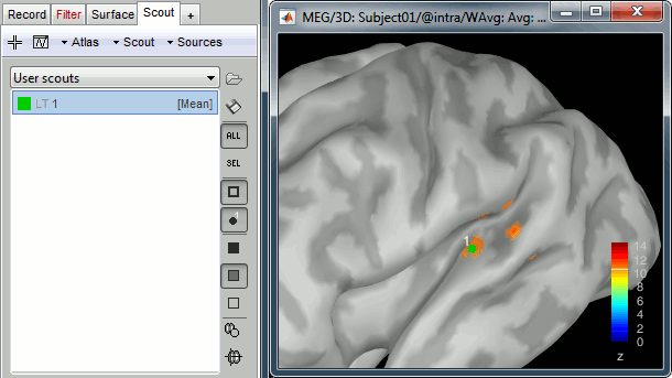
If you are not satisfied with the position of the vertex you selected, delete the new scout (select it in the list and press the Delete key, or menu Scout > Delete) and try again.
Rename it "A1L", for primary auditory left: double-click on it in the list, or menu Scout > Rename.
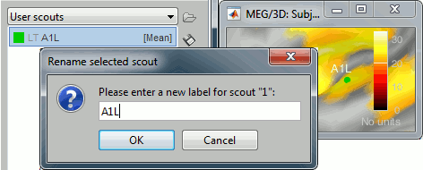
In light grey, you can see in the list the letters "LT", this means that based on the anatomical atlases imported from FreeSurfer, the point you clicked is in the left temporal lobe.
Growing a scout
For now, our scout contains only one vertex of the cortex surface. Most of the time, the aim of a scout is to extract the average activity over a larger region. The buttons in the Scout size section offer basic operations to define the scout extension.
[>]: Add the closest vertex (with respect to the seed) to the current scout.
[<]: Remove the furthest vertex (with respect to the seed) from the current scout.
[>>]: Grow scout in all directions.
[<<]: Shrink scout in all directions.
'Constrained': If this button is pressed, only the vertices that have a source value above the threshold will be added to the scout (its growth will be limited to the colored patch on the surface).
Add vertex manually: Select the Select point button, then select again the "A1L" scout. When you click on a vertex on the surface, it is added to the selected scout.
Remove vertex manually: Same as previously, but holding the SHIFT key at the same time.
Grow the scout A1L to 20 vertices, not in constrained mode. You can read the number of vertices and the estimated cortical area just below the [<<] and [>>] buttons.
Display time series
Select the scout in the list, click on the second button in the toolbar [Display scouts time series]. It displays the signal associated with this region for the entire time window (-100ms to 500ms).
We can now observe the early response at 50ms (P50) that was not very obvious before.
3D display options
In the toolbar on the right side of the scouts list, you can find a list of display options. Leave your mouse over each button for a few seconds to get a short description.
 Load Atlas
  Save selected scouts
  Show all the scouts
  Show only the selected scouts
 Hide all: Uncheck both buttons above to hide the scouts in the 3D figure.
 Show / hide the contour line
  Show / hide the scouts labels
  Scout patch: Opaque
  Scout patch: Transparent
  Scout patch: None
  Display the color of the region instead of the scout color (only for anatomical atlases)
  Center MRI on scout (open the MRI viewer and show the position of the scout's seed)
Scout function
We have extended the scout A1L to 20 vertices. Because this is a source model with constrained dipoles orientations, we have one source only per vertex. The region A1L corresponds to 20 signals.
The signals are grouped together into one unique signal that is then used to represent the activity of the region of interest. In the list of available scouts, you can see the indication [Mean] next to the name of the scout. It represents the name of the function that is used for combining all the source signals into one. This function can be changed individually for each scout, with the menu Scout > Set function.
Here is a description of the different options. In the case of unconstrained sources (3 signals for each vertex, one for each orientation), the function is applied separately for each orientation and produces 3 time series instead of one. For more details, see the code of bst_scout_value.m.
Mean: Average all the signals.

PCA: Take the first mode of the Principal Component Analysis decomposition of all the signals. Here, this is computed on a single file for display, but PCA works best when all epochs and conditions are processed together, through the process tabs. See PCA tutorial.
Fast PCA: Same as PCA function, but computes the first PCA decomposition based only on a subset of the strongest signals. It gives very similar results, but its computation is much faster for scouts that group a large number of dipoles (>50).

Mean(norm): Average the absolute values of all the signals: mean(abs(signal))

Max: For each time point, get the maximum across all the vertices.
Signed maximum: m = max(abs(signal)), scout = sign(signal(m)) * m

Power: Average the square of all the signals: mean(signal^2)

RMS: Square root of average the square of all the signals: sqrt(mean(signal^2))

All: Do not apply any operation on the scouts signals, returns all the signals.

Note that the function selected here is ignored when running a process with a scout function option, like "Extract > Scout time series" or Connectivity.
Option: Absolute / relative
As said in the previous tutorial, the minimum norm current amplitudes can be positive or negative depending on the dipole orientation. This means that the values of the scouts, depending on the function that is used, may be positive or negative too. Most of the time we are interested in visualizing the absolute values of the scouts time series, to compare the activation level in different conditions or subjects. But it is sometimes easier to understand the temporal dynamic of a ROI with the relative values.
At the bottom of the Scout tab, you can choose to display either Absolute or Relative values.
The effect of this options changes whether you are processing source files with constrained (1 signal per vertex) or unconstrained (3 signals per vertex) dipoles orientations:
Constrained: Apply the scout function to all source signals, then:
Absolute: abs(ScoutFunc(sources))

Relative: ScoutFunc(sources)

Unconstrained: Apply the scout function to the source signals for each orientation (Sx,Sy,Sz) separately, and then returns either the norm of the 3 orientations, or each orientation separately (except PCA, see below):
Absolute: Returns one time series:
sqrt( ScoutFunc(Sx)2 + ScoutFunc(Sy)2 + ScoutFunc(Sz)2)

Relative: Returns three time series:
A1L1=ScoutFunc(Sx), A1L2=ScoutFunc(Sy), A1L3=ScoutFunc(Sz)

- Since PCA can also be used to combine the 3 orientations, it is applied here across all sources and orientations at once, producing a single time series, like in the constrained case above.
Display only: Note that this relative/absolute selection is a display option, it is not saved in the scouts themselves. It is used only when displaying the scouts time series with the [Display scouts time series] button of the Scout tab. In all other cases, such as the extraction of the scouts values from a script, this relative/absolute option is ignored. In those cases, there may also be an option to flatten unconstrained source orientations first, resulting in a single time series per scout instead of 3.
Multiple conditions
We can easily compare the activity between multiple conditions and multiple regions of interest.
In Intra-subject, open at the same time the normalized sources for deviant and standard condition.
Select the scout A1L and click on [Display scouts time series].
This computes the scouts time series for all the files that are currently open.

Use the checkbox Uniform amplitude scale to configure the amplitude of multiple axes.
Select it to force multiple graphs to use the same scale, unselect it to scale each graph separately.

At the bottom of the Scout tab, select the option "Overlay: Files", then click [Display] again.

The Z-score value for the standard condition is a lot higher than the deviant condition because of the number of trials we used for computing the two averages (5x more trials for the standard). The SNR is higher with more trials, the baseline has less variance so the Z-score is higher.
To overlay the results of two conditions averaged with very different numbers of trials, it makes more sense to display the scout time series for non-normalized maps (averaged current density).

Other regions of interest
- Let's place all the regions of interest starting from the easiest to identify.
Open the normalized average source files (standard and deviant), together with the average recordings for the deviant and standard condition for Run#01 for an easier time navigation.
In the Surface tab, smooth the cortical surface at 70%.
- For each region: go to the indicated time point, adjust the amplitude threshold in the Surface tab, identify the area of interest, click on its center, grow the scout, rename it.
Grow all the regions to the same size: 20 vertices.
A1L: Left primary auditory cortex (Heschl gyrus) - Already marked.
- The most visible region in both conditions. Active during all the main steps of the auditory processing: P50, N100, MMN, P200, P300.
Standard condition, t=90ms, amplitude threshold=50%

A1R: Right primary auditory cortex (Heschl gyrus)
- The response in this region is not as obvious than A1L. These binaural auditory stimulations should be generating similar responses in both left and right auditory cortices at early latencies. Possible explanations for this observation:
- The earplug was not adjusted on the right side and the sound was not well delivered.
- The subject's hearing from the right ear is impaired.
- The response is actually stronger in the left auditory cortex for this subject.
- The orientation of the source makes it more difficult for the MEG sensors to capture.
Deviant condition, t=90ms, amplitude threshold=50%

- The response in this region is not as obvious than A1L. These binaural auditory stimulations should be generating similar responses in both left and right auditory cortices at early latencies. Possible explanations for this observation:
IFGL: Left inferior frontal gyrus (Brodmann area 44)
- Involved in the auditory processing, particularly while processing irregularities.
- You can use the atlas "Brodmann-thresh" available in the Scout tab for identifying this region.
Deviant condition, t=130ms, amplitude threshold=30%

M1L: Left motor cortex
- The subject taps with the right index when a deviant is presented.
- The motor cortex responds at very early latencies together with the auditory cortex, in both conditions (50ms and 100ms). The subject is ready for a fast response to the task.
- At 170ms, the peak in the standard condition probably corresponds to an inhibition: the sound heard is not a deviant, there is no further motor processing required.
- At 230ms, the peak in the deviant condition is probably a motor preparation. At 350ms, the motor task begins, the subject moves the right hand (recorded reaction times 500ms +/- 108ms).
- We cannot expect to have clear responses during the motor response because of the averaging. The response times are variable, so in order to get a better representation of the regions involved we should import and average the trials based on the response triggers.
Deviant condition, t=440ms, amplitude threshold=25%

Multiple scouts
We can display the activity of multiple regions simultaneously.
- Close everything (toolbar button [X]).
Open the two normalized average source files (standard and deviant).
In the Scout tab, select the A1L and IFGL scouts simultaneously.
Select the option "Overlay:Scouts", do not select "Overlay:Files", Absolute values.
Click on [Display scouts time series].

Now select the option "Overlay:Files", do not select "Overlay:Scouts", click on [Display].

In both conditions, we observe similar early responses (P50 and N100), then it diverges.
In the deviant condition, we observe a pattern A1-IFG-A1 that is absent in the standard condition.
From the database explorer
You have to display the sources on the cortex to create the scouts. But once they are created, you can directly display the scouts time series from the database explorer. It means that you can quickly compare the values for a scout between many different conditions without having to open them all.
- Close everything (toolbar button [X]).
Select the option "Overlay:Files", do not select "Overlay:Scouts".
Select the two average recordings in Run#01 folder > right-click > Scouts time series.
Note that this menu is present at all the levels in the database explorer.
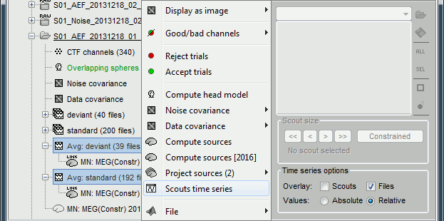
If no scout is currently loaded in the Scout tab, it shows all the scouts available in the surface.
If a surface is loaded, and at least one scout selected in the Scout tab, this popup menu would display only the selected scouts.
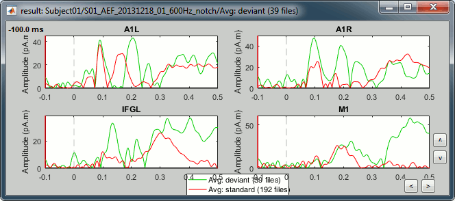
Once the list of scouts is loaded in the Scout tab, you can select one of them, and then display its values for all the trials of a single condition (overlay:files).
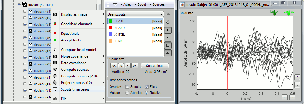
Sign flip
In the case of source models with constrained orientations (normal to the cortex), the sign of the current can be an issue. If the region is large enough to include vertices with normals in opposite directions, averaging the source values may cancel out the activity.
Let's use the example from the previous tutorial and consider that one scout contains all the dipoles corresponding to both the red arrows (positive values) and the blue arrows (negative values). If we average all the values from this scout, we get a value close to zero.
To avoid this, a mechanism was added in the scout calculation, to flip the sign of sources with opposite directions before the averaging. We start by finding the dominant orientation of the scout, then flip the sign of the values that are not in the same direction (scalar product of the orientations < 0).
If the sign of some sources is flipped, you get a message in the Matlab command window, for example:
BST> Flipped the sign of 7 sources.
Scout toolbar and menus
Menu: Atlas
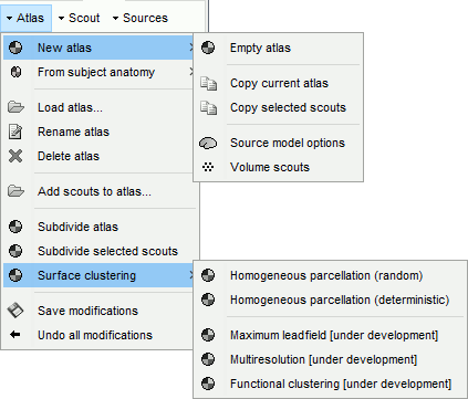
New atlas:
Empty atlas: Create a new empty atlas.
Copy atlas: Duplicate an atlas and all the scouts it contains.
Copy selected scouts: Create a new atlas and copy only the selected scouts to it.
Source model options: Create a special atlas "Source model", with which you can attribute different modeling constraints to each region, after merging the cortex with some subcortical regions. This is required to use the option "Custom head model" (mixed models).
Volume scouts: Create a volume atlas in order to define 3D scouts (volume head models).
From subject anatomy: Import as surface or volume scouts the ROIs defined in one of the volume parcellation available in the subject's anatomy (MNI-based atlases or subject parcellations from CAT12 or FreeSurfer).
Load atlas: Load ROIs or a cortical parcellation coming from FreeSurfer or BrainSuite as a new atlas.
Rename atlas: Change the name that appears in the atlas list to refer to the selected atlas.
Delete atlas: Delete the current atlas and all the scouts in contains.
Add scouts to atlas: Load ROIs or a cortical parcellation and add them to the current atlas.
Subdivide atlas: Splits all the scouts of the current atlas in smaller ROIs. Available options:
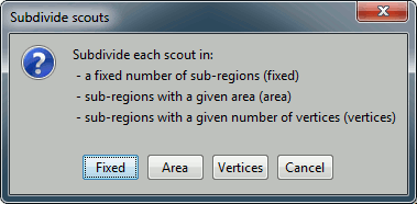
Subdivide selected scouts: Same thing, but processes only the selected scouts.
Surface clustering: Create a parcellation of the cortex surface and saves it as a new atlas.
Only the "Homogeneous parcellation" clustering is currently available.Save modifications: Force the current modifications to be saved to the cortex surface.
Undo all modifications: Restore the atlas the way it was the last time the surface was loaded.
Menu: Scout
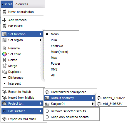
New: coordinates: Create a new scout starting from the vertex that is the closest to the specified coordinates. You can enter coordinates in MRI, SCS or MNI coordinates.
Add vertices: The user can select some points on the cortex surface and add them to the scout.
Equivalent: Click on Select point (first toolbar button) then select the scout in list.Edit in MRI: Open an interface to edit the selected scout as a 3D ROI, slice by slice. Only the vertices contained in the 3D mask are kept, all the volume information is lost. It means that the mask you intended to draw might be very different from what you get as a scout at the end. This is not a very reliable tool, as there is no direct correspondence between the volume and the surface.
Set function: Set the scout function for the selected scouts.
Set region: Set the cortical region for the selected scouts.
Rename: Rename the selected scout. Shortcut: double-click.
Set color: Change the display color of the selected scout.
Delete: Delete selected scouts. Shortcut: Delete key
Merge: Join two or more selected scouts.
Duplicate: Duplicate selected scouts.
Difference: With two scouts A and B selected, this menu removes the vertices included scouts A from scout B, or vice versa. The direction of the difference is asked in a dialog window.
Intersect: With two or more scouts selected, this menu creates a new scout with the vertices that are common for all the selected scouts.
Export to Matlab: Export the structures of the selected scouts to the Matlab environment and makes them accessible from the command window. This menu can be useful to get quickly the list of vertex indices or modify a scout manually.
Import from Matlab: Import scouts structures that you modified manually from your Matlab command window directly as new scouts.
Project to: Project the selected scout on another surface available in the database.
Project to: Contralateral hemisphere: Transfer scouts defined on one hemisphere to the other hemisphere. This feature is only available with FreeSurfer, and the recon-all segmentation pipeline must be executed with additional options. In the anatomy of the tutorial dataset, this option was not used, and therefore this menu generates an error. However, this option was used in the in the ICBM152 2023b template anatomy. To get this contralateral projection to work, FreeSurfer recon-all must be executed again with the extra option, and the anatomy of the subject must be imported again. More information.
Edit surface: Create a new surface containing only the desired parts (remove or keep only the selected scouts). This is useful for instance for selecting one sub-cortical region from the Aseg FreeSurfer atlas (see the FreeSurfer tutorial).
Export as MRI mask: Create a MRI mask/parcellation using selected scouts (all scouts are used if none is selected). For volume scouts, they are projected from the source grid to the MRI volume. For surface scouts, their cortex patch is projected to the MRI volume, this is based on the registration of the cortical surface and MRI volume.
Menu: Sources
Correlation with sensor: Create a new scout with all the sources that are strongly correlated with a given sensor.
Expand with correlation: Computes the correlation between the values for the scout's seed (first point) and all the other sources. The sources that have correlation coefficient superior to a given threshold are added to the scout.
Maximal value (new scout): Find the vertex with the maximal intensity at the current time, and create a scout centered on it.
Maximal value (selected scout): Move the scout's seed to the source that has the maximum amplitude in the scout, at the current time.
Simulate recordings: Multiply the selected scouts with the forward model. Simulate the scalp data that would be recorded if only the selected cortex region was activated; all the other sources are set to zero. Create a new data file in the database.
If no scout selected: simulate recordings produced by the activity of the entire cortex.
Scout region
A scout is defined by its name, and it has several properties: a list of vertices and an aggregating function. These are usually enough to explore the activity at the cortex level the way we did it in these tutorials. An extra property can be defined on the scout: the explicit classification in a brain region. This property is used only in more advanced functional connectivity analysis, for the representation of the NxN connection graphs. It is introduced here for reference purpose.
A brain region in Brainstorm is following a hierarchy with three levels: hemisphere / lobe / sub-region. The definition at each level is optional: a region can be classified only at the hemisphere level, or at the hemisphere+lobe level, or none of them. It depends on level or hierarchy you are interested in to explore the connectivity graphs.
The region for a scout can be set with the Scout > Set region menus, and is encoded in a string that contains at least 2 characters: "HLxxx". H represents the hemisphere (L,R,U), L stands for the lobe (F,PF,C,P,T,O,L,U), and xxx for the sub-region name (optional). For both the hemisphere and the lobe, the value "U" stands for "Undefined", meaning that the classification is simply not set. The menu Set region>Custom region... lets you directly edit this string.
When set, the region string is shown before the scout name in the list, representing only the defined levels. It doesn't show the letters U for "undefined".
On the hard drive
The scouts are saved in the surface file on which they have been defined.
In the anatomy view, right-click on the selected cortex surface (cortex_15002V) > View file contents.
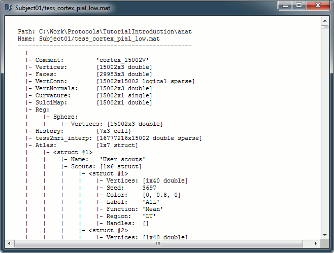
iAtlas: Index of the atlas that is currently selected for this surface.
Atlas: Array of structures, each entry is one menu in the drop-down list in the Scout tab.
Name: Label of the atlas (reserved names: "User scouts", "Structures", "Source model").
Scouts: Array of structures, one per scout in this atlas.
Vertices: Array of indices of the vertices that are part of the scout.
Seed: Index of the central point of the scout (or the most relevant one).
Color: [r,b,g] color array, with values between 0 and 1.
Label: Display name of the scout (must be unique in this atlas).
Function: Scout function {'Mean', 'PCA', 'FastPCA', 'Mean_norm', 'Max', 'Power', 'All'}
Region: Code name for indicating the anatomical region in which the scout is located.
Handles: Graphic handles if the scout is currently displayed (always empty in a file).
Useful functions
bst_scout_value: Combine multiple signals into one.
process_extract_scout: Process "Extract > Scouts time series"
view_scouts: Compute scouts time series and displays them in a new figure.
Additional documentation
Forum: Scout coordinates: http://neuroimage.usc.edu/forums/showthread.php?2375
Forum: Coordinates of the max value from a scout: https://neuroimage.usc.edu/forums/t/get-the-coordinates-of-a-max-value-from-scouts/4959/2
Forum: Importing other FreeSurfer atlases: https://neuroimage.usc.edu/forums/t/930
Tutorial 24: Time-frequency
Authors: Francois Tadel, Dimitrios Pantazis, Elizabeth Bock, Sylvain Baillet
This tutorial introduces how to compute time-frequency decomposition of MEG/EEG recordings and cortical currents using complex Morlet wavelets and Hilbert transforms.
Contents
- Introduction
- Morlet wavelets
- Edge effects
- Simulation
- Process options
- Display: Time-frequency map
- Display: Mouse and keyboard shortcuts
- Display: Power spectrum and time series
- Normalized time-frequency maps
- Tuning the wavelet parameters
- Hilbert transform
- MEG recordings: Single trials
- Display: All channels
- Display: Topography
- Scouts
- Full cortical maps
- Unconstrained sources
- Getting rid of the edge effects
- On the hard drive
- Additional documentation
Introduction
Some of the MEG/EEG signal properties are difficult to access in time domain (graphs time/amplitude). A lot of the information of interest is carried by oscillations at certain frequencies, but the amplitude of these oscillations is sometimes a lot lower than the amplitude of the slower components of the signal, making them difficult to observe.
The averaging in time domain may also lead to a cancellation of these oscillations when they are not strictly locked in phase across trials. Averaging trials in time-frequency domain allows to extract the power of the oscillation regardless of the phase shifts. For a better understanding of this topic, we recommend the lecture of the following article: Bertrand O, Tallon-Baudry C (2000), Oscillatory gamma activity in humans: a possible role for object representation.
In Brainstorm we offer two approaches for computing time-frequency decomposition (TF): the first one is based on the convolution of the signal with series of complex Morlet wavelets, the second filters the signal in different frequency bands and extracts the envelope of the filtered signals using the Hilbert transform.
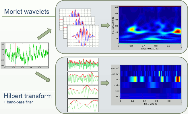
Morlet wavelets
Complex Morlet wavelets are very popular in EEG/MEG data analysis for time-frequency decomposition. They have the shape of a sinusoid, weighted by a Gaussian kernel, and they can therefore capture local oscillatory components in the time series. An example of this wavelet is shown below, where the blue and red curves represent the real and imaginary part, respectively.
Contrary to the standard short-time Fourier transform, wavelets have variable resolution in time and frequency. For low frequencies, the frequency resolution is high but the time resolution is low. For high frenqucies, it's the opposite. When designing the wavelet, we basically decide a trade-off between temporal and spectral resolution.
To design the wavelet, we first need to choose a central frequency, ie. the frequency where we will define the mother wavelet. All other wavelets will be scaled and shifted versions of the mother wavelet. Unless interested in designing the wavelet at a particular frequency band, the default 1Hz should be fine.
Then, the desirable time resolution for the central frequency should be defined. For example, we may wish to have a temporal resolution of 3 seconds at frequency 1 Hz (default parameters). These two parameters, uniquely define the temporal and spectral resolution of the wavelet for all other frequencies, as shown in the plots below. Resolution is given in units of Full Width Half Maximum of the Gaussian kernel, both in time and frequency.
Edge effects
Users should pay attention to edge effects when applying wavelet analysis. Wavelet coefficients are computed by convolving the wavelet kernel with the time series. Similarly to any convolution of signals, there is zero padding at the edges of the time series and therefore the wavelet coefficients are weaker at the beginning and end of the time series.
From the figure above, which designs the Morlet wavelet, we can see that the default wavelet (central frequency fc=1Hz, FWHM_tc=3sec) has temporal resolution 0.6sec at 5Hz and 0.3sec at 10Hz. In such case, the edge effects are roughly half these times: 300ms in 5Hz and 150ms in 10Hz.
More precisely, if f is your frequency of interest, you can expect the edge effects to span over FWHM_t seconds: FWHM_t = FWHM_tc * fc / f / 2. Examples of such transients are given in the figures below.
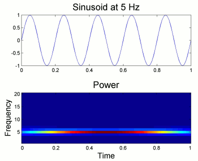
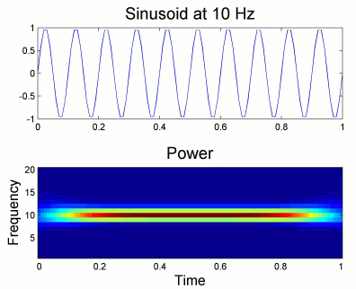
We also need to consider these edge effects when using the Hilbert transform approach. The band-pass filters used before extracting the signal envelope are relatively narrow and may cause long transients. To evaluate the duration of these edge effects for a given frequency band, use the interface of the process "Pre-process > Band-pass filter" or refer to the filters specifications (tutorial #10).
Simulation
We will illustrate the time-frequency decomposition process with a simulated signal.
The following code generates a sum of three sinusoids (2Hz, 20Hz, 50Hz) with random white noise. The 50Hz and noise are present everywhere, the 2Hz and 20Hz start only after two seconds.
f1 = 2; f2 = 20; f3 = 50;
i =2000:6000;
Data(1,i) = sin(f1*2*pi*t(i)) + 0.4 * cos(f2*2*pi*t(i));
Data = Data + 0.2 * sin(f3*2*pi*t) + 0.4 * rand(1,6000);
Empty the Process1 list (right-click > Clear list) then click on [Run].
Run process: Simulate > Simulate generic signals.
Ntime=6000, Sampling frequency=1000Hz (signal duration = 6000/1000 = 6 seconds).
Copy-paste the few lines of code above to generate the sum of three sinusoids.
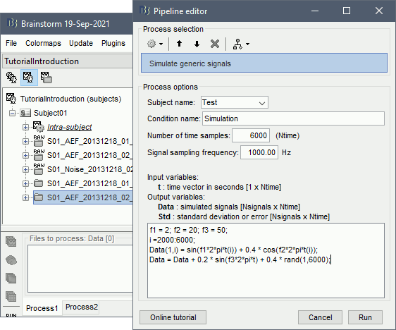
Double-click on the new file to look at the simulated signal.

- In Process1, select the simulated signal.
Run process: Frequency > Time-frequency (Morlet wavelets).
Select the option Spectral flattening: The normalization will be discussed later.
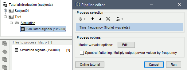
Click on the button [Edit] to see all the process options.
Time definition: Same as input, Frequency definition: Linear 1:1:60, Compute measure: Power.
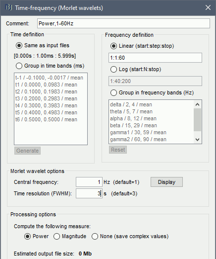
Process options
Comment: String that will be displayed in the database explorer to represent the output file.
Time definition
Same as input file: The output file has the same time definition as the input file.
In this example, it means: 6000 samples between 0 and 6s.Group in time bands: This option adds a step of computation. First it computes the TF decomposition for all the input file, then averages the power by time band. To define a time band:
Enter your own time bands in the text area, one line per time band, with the following format: "name / time definition / function"
- Click on the button [Generate] to automatically create a list of time bands with the same length. You will be asked the maximal length of each time band.
The function is the measure we take to combine the values for all the individual frequencies into one for the frequency band. Possible values are: mean, max, std, median.
Frequency definition: Frequencies for which the power will be estimated at each time instant.
Linear: You can specify the frequencies with the Matlab syntax start:step:stop.
The default is "1:1:60", which produces 60 values [1, 2, 3, 4, ..., 59, 60].Log: With the option start:N:stop, produces a list of N frequencies logarithmically scaled between "start" and "stop". For example "1:40:80" is converted to [1, 1.5, 2.1, 2.7, ..., 61.5, 65.8, 75, 80]
Group in frequency bands: As for the time definition, this option leads to a two-step process. First it computes the TF decomposition for several values in the frequency band, then it averages the power of TF coefficients per frequency band. To define a frequency band:
One line per frequency band, with the format "name / frequency definition / function"
The frequency definition is a Matlab expression evaluated with an eval() call. If the frequency definition contains only two values, Brainstorm adds two extra values in the middle so that the final averaged value is a bit more robust. Example of valid expressions:
"2,4": Evaluates to [2,4], and then expands to the frequency vector [2, 2.66, 3.33, 4]
"2:0.5:4": Evaluates to [2 2.5 3 3.5 4]
"2, 2.5, 3, 3.5, 4": Evaluates to [2 2.5 3 3.5 4]The function is the measure we take to combine the values for all the individual frequencies into one for the frequency band. Possible values are: mean, max, std, median.
Morlet wavelet options
Central frequency: Frequency where the mother wavelet is designed. All other wavelets will be shifted and scaled versions of the mother wavelet
Time resolution (FWHM): Temporal resolution of the wavelet at the central frequency (in units of Full Width Half Maximum). Click [Display] to see the resolution of the wavelet for other frequencies.
Compute the following measure:
The convolution of the signal with complex Morlet wavelets returns the complex coefficients for each frequency/time/sensor. Typically, what we display is the power of the coefficients (square of the amplitude: abs(TF)2). You can choose if you want to apply this transformation or not.
Power: Computes the "power" transformation immediately after the TF decomposition. This discards the phase information, but produces files that are twice smaller and a lot easier to process.
Magnitude: Save the magnitude of the complex values instead of the power: abs(TF).
None: Save the TF coefficients as they are computed (complex values). This can be useful if you plan to use these decompositions for other purposes that require the phase.
- Some combinations of options may disable this choice. If you select frequency bands, the program will have to compute the power before averaging the values, therefore "none" is not an option.
Display: Time-frequency map
Right on the new time-frequency file > Time-freq: One matrix (same as double-clicking).
This menu displays the time-frequency decomposition of the first (and only) signal. The Brainstorm window shows two new elements: the tab "Display" and the frequency slider.

- We can easily identify the three horizontal bars as the three sinusoids in the simulated signals, and the trade-off between accuracy in time and accuracy in frequency. Set the measure to "magnitude" in the Display tab if you don't. Click on the figure to move the time-frequency cursor and explore the two axes of the plane.
2Hz: High frequency resolution but poor time resolution (supposed to start sharply at 2s)
20Hz: Better time resolution but poorer frequency resolution (17-24Hz)
50Hz: Continuous over the 6s - Frequency resolution gets even worse (40-60Hz). It looks discontinuous because this oscillation has the same amplitude as the white noise we added in the signal (weight 0.4, relatively to the 2Hz oscillation).
Current frequency: Slider that shows the current frequency selected in all the figures.
Just like the time, the frequency selection is centralized and managed by one control only for all the figures. As a consequence, it is impossible to display TF files with different frequency definitions at the same time. This can be perceived as an annoying limitation, but it allows all the simultaneous displays to be consistent at anytime and makes the interface more intuitive to manipulate, with lower risks of mistakes in the interpretation of the different figures.List of signals: This drop-down list shows the signal currently displayed in the selected figure. In this case, there is only one channel of data called "s1". It will be more useful later.
Hide edge effects: When this option is selected, the time-frequency coefficients that could not be properly estimated because of a lack of time samples are hidden. It allows you to see only the information that is really reliable. The lower the frequency, the longer the edge effects. In the screen capture below, the colormap has been changed to "jet" and the maximum set manually to 0.2 (measure=power).
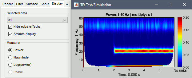
Smooth display: Re-interpolates the time-frequency maps on a finer grid to produce nicer plots.
Measure: Type of measure that is currently represented in the selected figure. The entries that are enabled depend on the type of data that is saved in the file. In this case, we saved directly the power of the wavelet coefficients in the file, we discarded the angle/phase information, so the "phase" option is disabled. The other options are: Magnitude = sqrt(power), Log = 10*log10(power)
Colormap: As explained in the previous tutorials, you can change the colormap by clicking+moving on the colorbar on the right of the figure. Double-click on the colorbar to restore the defaults.
Display: Mouse and keyboard shortcuts
Mouse shortcuts
Left-click: Selection of current time and frequency.
Left-click + move: Select a time/frequency range. The legends of the X/Y axis show the selection.
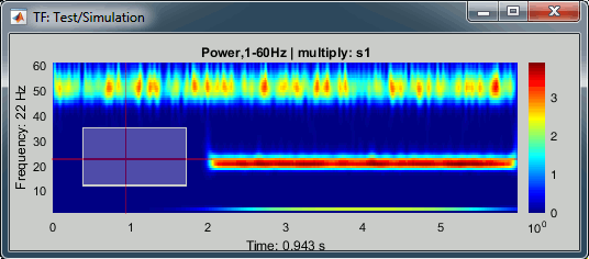
Mouse wheel: Zoom in time, centered on the current time cursor.
Control + mouse wheel: Zoom in frequencies, centered on the current frequency cursor.
Right-click + move, or Control + left-click + move: Move in the zoomed image.
Double-click: Restore initial view.
Keyboard shortcuts:
Left/right arrows: Change the current time.
Page-up/page-down: Change the current time, 10 time samples at a time.
Up/down arrows: Change the the sensor displayed in this figure.
Control + up/down arrows: Change the current frequency.
Enter: View the original time series for this sensor.
Control + R: View the original MEG recordings.
Control + T: View the time-frequency 2D topography.
Control + I: Save as image.
Control + D: Dock figure in the Matlab environment.
Figure popup menu
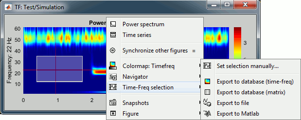
Set selection manually: Does the same thing as drawing a time/freq selection square on a figure, but by typing the values for time and frequency manually.
Export to database: Save the selection for the displayed sensor in a new file in the database.
Export to file: Same as "Export to database", but the saved file is not registered in the database.
Export to Matlab: Same as "Export to database", but the output structure is sent to a variable in the Matlab base workspace instead of being saved to a file.
Display: Power spectrum and time series
Right-click on the file in the database or directly on the time-frequency figure to access these menus.
Power spectrum: For the current time, shows the power for all the frequencies.
Time series: For the current frequency, shows the power for all the time samples.
Example: Power spectrum density at 0.5s and power time series at 2Hz.
We see the oscillation at the 50Hz in the PSD plot, and the oscillation at 2Hz in the TS plot.
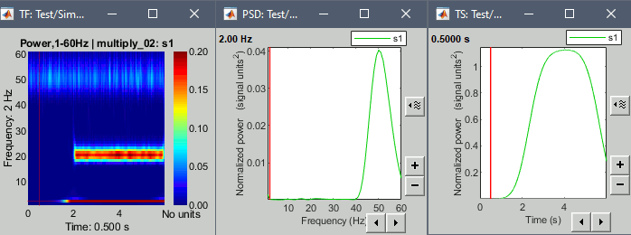
Example: Power spectrum density at 4s and power time series at 20Hz.
We see all three oscillations in the PSD plot, and the oscillation at 20Hz in the TS plot.
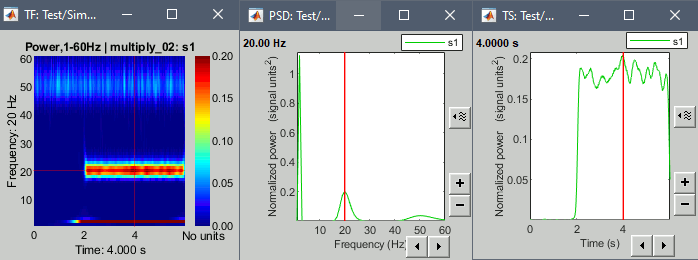
Note that if you right-click on the file in the database explorer and then select one of these menus, it will show all the signals. If you right-click on an existing time-frequency figure, it will show only the selected signal. It doesn't make any difference here because there is only one signal, but it will with the MEG recordings.
Normalized time-frequency maps
The brain is always active, the MEG/EEG recordings are never flat, some oscillations are always present in the signals. Therefore we are often more interested in the transient changes in the power at certain frequencies than at the actual power. A good way to observe these changes is to compute a deviation of the power with respect with a baseline.
There is another reason for which we are usually interested in standardizing the TF values. The power of the time-frequency coefficients are always lower in the higher frequencies than in the lower frequencies, the signal carries a lot less power in the faster oscillations than in the slow brain responses. This 1/f decrease in power is an observation that we already made with the power spectrum density in the filtering tutorial. If we represent the TF maps with a linear color scale, we will always see values close to zero in the higher frequency ranges. Normalizing each frequency separately with respect with a baseline helps obtaining more readable TF maps.
No normalization
The values we were looking at were already normalized (checkbox "Spectral flattening" in the process options), but not with respect to a baseline. We will now compute the non-normalized power obtained with the Morlet wavelets and try the various options available for normalizing them.
- In Process1, keep the simulated signal selected.
Run process: Frequency > Time-frequency (Morlet wavelets), No spectral flattening.
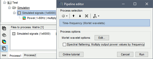
Double-click on the file. As expected, we only see the lower frequencies in this representation: the power of the 2Hz oscillation is a lot larger than the power at 20Hz or 60Hz.
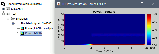
Spectrum normalization
- In Process1: Select this new non-normalized file "Power,1-60Hz".
Run process: Standardize > Spectrum normalization, Method=1/f compensation.
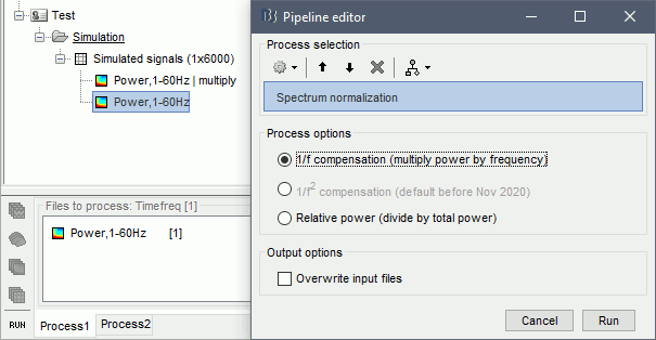
This produces exactly the same results as previously (option "Spectral flattening" in the time-frequency process). It multiplies the power at each frequency bin with the frequency value (eg. multiplies by 20 the power at 20Hz), in order to correct for the 1/f shape we observe in the power spectrum. This works well for the lower part of the spectrum and up to 60-80Hz, but past this range it tends to overcompensate the higher frequencies.
Note that it does not do any form of baseline correction: the 50Hz oscillation is visible everywhere.
Baseline normalization
The second way to proceed is to normalize the power with respect to its average level during a reference time period. We can consider the oscillations at 2Hz and 20Hz as our events of interest, and the 50Hz as noise we want to get rid of. The segment from 0 to 2 seconds does not contain any of the signals of interest, therefore we can consider it as a baseline.
However, we will not be able to use the full segment [0,2]s because of the edge effects we described at the beginning of this tutorial. The time-frequency map at 2Hz with the display option "Hide edge effects" (left figure below) shows that the power could not be estimated correctly before 0.75s, therefore we shouldn't use it as a baseline. The power time series at 2Hz (right) shows that the power related with the 2Hz oscillation starts to increase significantly after 1.25s, therefore it's not really a "baseline" anymore. This leaves only the segment [0.75,1.25]s available.
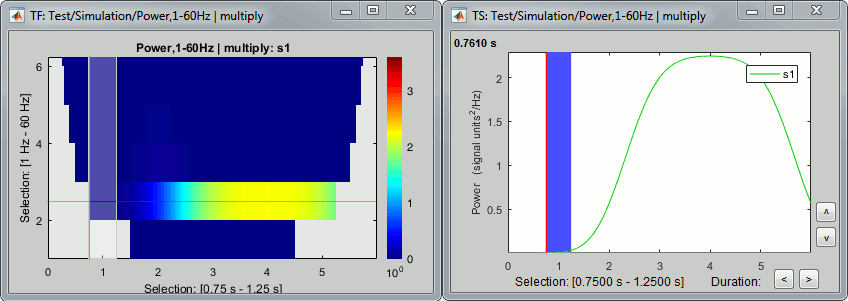
At 20Hz, the expected transient effects are only 75ms long, therefore we could use a much longer baseline if we were not interested by the lower frequencies: [0.075, 1.925]s.
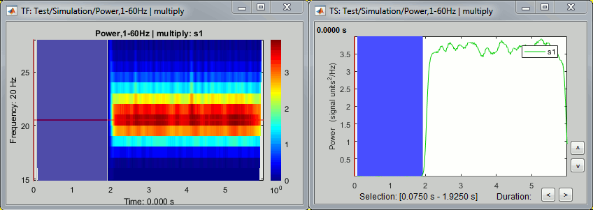
In this case, we have a very long "resting" time segment (2s), therefore the edge effects are not a problem for picking a time window for the baseline normalization. We will use the first time window mentioned, [0.75,1.25]s as it is long enough (500ms) to estimate the baseline mean power. In real-life cases, with shorter epochs, it is sometimes difficult to find an acceptable trade-off between the baseline duration and the exclusion of the edge effects, especially for the lower frequencies.
Run process: Standardize > Baseline normalization, Baseline=[0.75, 1.25]s.
Method=Event-related perturbation: ERS/ERD stands for "event-related synchronization / desynchronization", a widely used normalization measure for time-frequency power maps. It evaluates the deviation from the mean over the baseline, in percents: (x-mean)/mean*100.
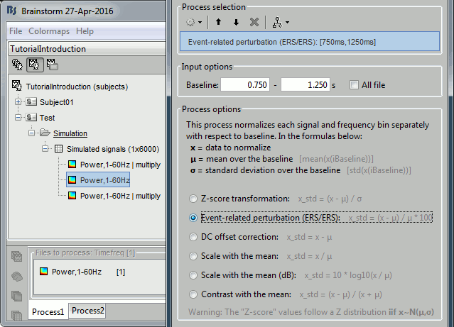
Double-click on the new "ersd" file. The colormap type changed from "Timefreq" to "Stat2", which uses by default the "rwb" color set and shows relative values. Indeed, the ERS/ERD values can be positive or negative: the power at a given time sample can be higher or lower than the average level during the baseline. In the simple simulation we used, there is no power decrease at any frequency after 2s, so the strong values are mostly positive. However, if you look in the file, you would see that there are many small negative values (due to the random noise we added).
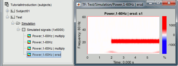
Note that the 50Hz disappeared because it was present during the baseline, while the 2Hz and 20Hz oscillations show high positive values (between 100% and 2000% increase from baseline).
Remember to select your baseline very carefully according to the frequency range you are interested in. See below examples obtained with different baselines: 0.075-1.925s, 0-2s, 0-6s.
Change the colormap to "jet" if you prefer, and adjust the colormap contrast as needed.

This video may help you understand better what are the implications of the baseline selection: http://www.mikexcohen.com/lecturelets/whichbaseline/whichbaseline.html
Tuning the wavelet parameters
Time resolution
You can adjust the relative time and frequency resolution of your wavelet transformation by adjusting the parameters of the mother wavelet in the options of the process.
Increasing the option "time resolution" will produce longer wavelets at a given frequency, hence increase the frequency accuracy (lower Δf) and decrease the time accuracy (higher Δt). Expect longer edge effects.
Decrease the time resolution will produce shorter wavelets at a given frequency, hence decrease the frequency accuracy (higher Δf) and increase the time accuracy (higher Δt). Expect shorter edge effects.
You can modify one or the other parameter, what is important is the product of the two. All the following combinations fc/FWHM_t produce the same results because their product is constant: (1Hz,3s), (3Hz,1s), (6Hz,0.5s), (60Hz,0.05s)

Examples for a constant central frequency of 1Hz with various time resolutions: 1.5s, 4s, 10s.
Frequency axis
You can also obtain very different representations of the data by changing the list of frequencies for which you estimate the power. You can change this in the options of the process.
Examples: Log 1:20:150, Log 1:300:150, Linear 15:0.1:25
Hilbert transform
We can repeat the same analysis with the other approach available for exploring the simulated signal in the time-frequency plane. The process "Frequency > Hilbert transform" first filters the signals in various frequency bands with a band-pass filter, then computes the Hilbert transform of the filtered signal. The magnitude of the Hilbert transform of a narrow-band signal is a measure of the envelope of this signal, and therefore gives an indication of the activity in this frequency band.
No normalization
Let's compute the same three results as before: non-normalized, spectral flattening, baseline normalization.
- In Process1, select the simulated signal.
Run process: Frequency > Hilbert transform, No spectral flattening, Do not mirror.
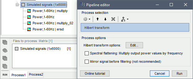
In the advanced options panel, keep the default options: Default frequency bands and Power.
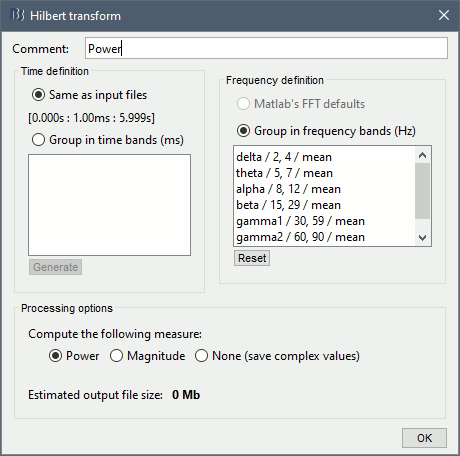
Double-click on the new file. The figure now has only 6 rows, one for each frequency band.
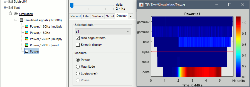
- The non-normalized results are already easy to interpret:
delta (2-4Hz): Includes the 2Hz oscillation, contribution starts at 2s
beta (15-29Hz): Includes the 20Hz oscillation, contribution starts at 2s
gamma1(30-59Hz): Includes the 50Hz oscillation, contribution starts at the beginning (0s)
Right-click on the file or figure > Time series. Example for delta and beta.

Normalization
- In Process1, select the non-normalized Hilbert-based decomposition.
Run process: Standardize > Spectrum normalization, Method=1/f compensation.
Run process: Standardize > Baseline normalization, Baseline=[0.75, 1.25]s, Method=ERS/ERD.
Display the two normalized files side by side.

Method specifications
Band-pass filters: Same filters as in the process "Pre-process > Band-pass filter", with the option "Stop-band attenuation: 60dB". For details, see the tutorial Power spectrum and frequency filters.
Edge effects: To estimate the duration of the transient effects for each frequency band, select the process "Band-pass filter", enter the frequency band of interest and click "View filter response". Example for the alpha band:
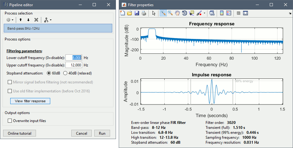
Hilbert transformation: Using the Matlab's hilbert() function.
Extraction of the envelope: Power of the complex Hilbert transform, abs(hilbert(x))2.
MEG recordings: Single trials
Let's go back to our auditory oddball paradigm and apply the concepts to MEG recordings. We will use all the trials available for one condition to estimate the average time-frequency decomposition.
Spectrum normalization
In Process1, select all the deviant trials in Run#01.
Run process: Frequency > Time-frequency (Morlet wavelets), No spectral flattening.
In the advanced options, select: Log 1:40:150, Power, Save average time-frequency maps.
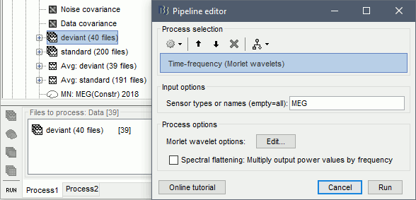
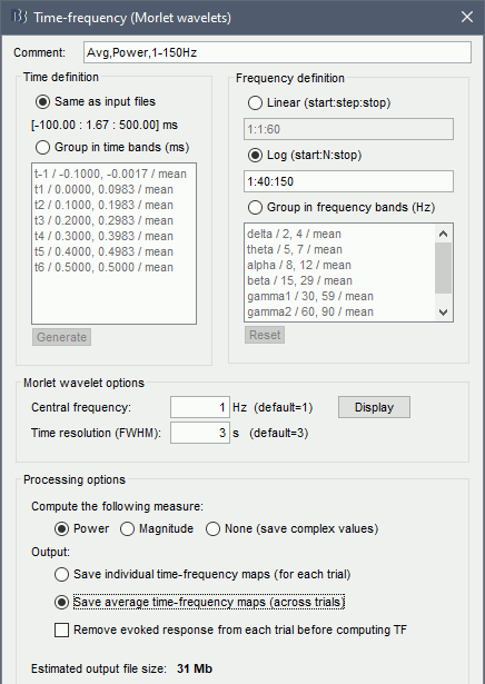
Save individual TF maps: This option stops the computation here and saves in the database one time-frequency file for each input file (40 files), with one TF map for each scout.
Save average TF maps: Instead of saving the TF for each file separately, it automatically computes the average of the power of all the TF. This is a good choice if you do not plan to use independently all the TF files, because it saves a lot of time and disk space.
Remove evoked response from each trial before computing TF: This option first computes the average of all the trials, then subtracts this average from each trial before computing the time-frequency decomposition. This brings the signals to a slightly more stationary state, which may help for the evaluation of the frequency contents.
Baseline normalization
Double-click on the new file Avg,Power,1-150Hz (MEG). Select "Hide edge effects".
In the drop-down list, select sensor MLP56 (the one with the strongest respons at 90ms).
Right-click on the TF figure > Time series.

Defining a baseline is now a lot trickier than with 6s-long simulated signal. The epochs are only 600ms long, and the power at many frequencies could not be estimated correctly. If we want all the values to be "good" after 0s, we cannot use anything below 15Hz. If we want to normalize the values, we have to go even higher: 30Hz if we want a baseline of 50ms before 0.
The epochs we use in this tutorial are too short to perform a correct time-frequency analysis. We should have imported at least 200ms more on each side, just for controlling the edge effects. You should always think carefully about the length of the epochs you import in your database if you are planning to run any form of frequency or time-frequency analysis.
- For the purpose of illustrating the tools available in Brainstorm, we will keep on working with these short epochs. Let's try to do the best we can with what we have here. We could use a baseline of 50ms to get a correct estimation above 30Hz, but this is probably a bit too short. We propose to include some more of the baseline (75ms), hoping there are not major edge effects in this segment.
- In Process1, select the average time-frequency file.
Run process: Standardize > Baseline normalization, Baseline=[-75, 0]ms, Method=ERS/ERD.
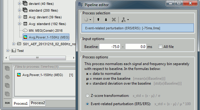
The new menus available to display this file are described in the next section.

Things to avoid
Avoid computing the time-frequency decomposition of the average of the trials, you would miss some of the induced response, the brain activity in higher frequencies that is not strictly time-locked to the stimulus, and not aligned in phase across trials. Always prefer the computation of the average of the time-frequency power maps of each trials, as we did here.
This is well documented in: Bertrand O, Tallon-Baudry C (2000).Avoid using the Hilbert transform approach on short recordings or averages, always use the wavelet approach in these cases. The band-pass filters used for the lower frequency bands may have very high orders, leading to long transients. The example below shows the expected transients for the default frequency bands using the process "Frequency > Hilbert transform", they can be much more invalidating than with the process "Frequency > Time-frequency (Morlet wavelets)".
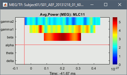
Display: All channels
Three menus display the time-frequency of all the sensors with different spatial organizations. All the figures below represent the ERS/ERD-normalized average. They use the "jet" colormap, which is not the default configuration for these files. To get the same displays, change the colormap configuration:
right-click on the figure > Colormap: Stat2 > Colormap > jet.
All channels: All the maps are displayed one after the other, in the order they are saved in the file.
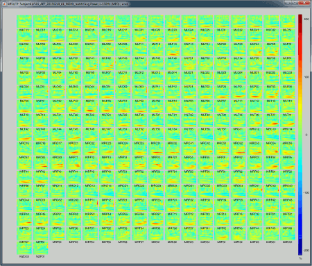
2D Layout (maps): Show each TF map where the sensor is located on a flattened 2D map. Most display options are available, such as the colormap management and the option "Hide edge effects".
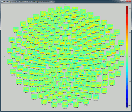
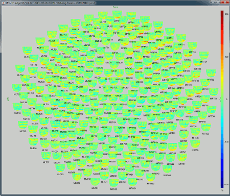
2D Layout (no overlap): Similar to the the previous display, but the positions of the images are reorganized so that they do not overlap.
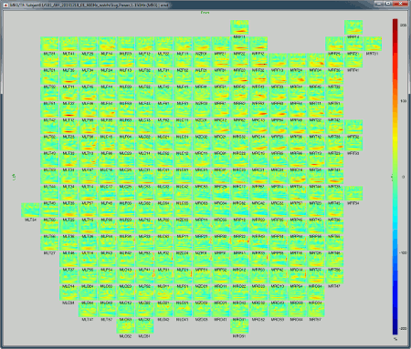
Image [channel x time]: Shows the values of all the sensors over time for one frequency.
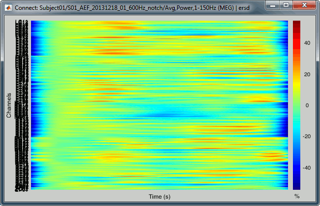
Useful shortcuts for the first three figures:
Click: Clicking on any small TF image opens a new figure with only the selected sensor.
Shift + click: Opens the original recordings time series of the selected sensor, when available. Here, we display an average of time-frequency maps, so this menu has no effect.
Mouse wheel: Zoom in/out.
Right click + move: Move in a zoomed figure.
Display: Topography
The menus below show the distribution of TF power over the sensors, for one time point and one frequency bin, very similarly to what was introduced in tutorial Visual exploration.
2D Sensor cap / 2D Disc / 3D Sensor cap: 175ms, 8Hz

2D Layout: 8Hz (black), 35Hz (white)
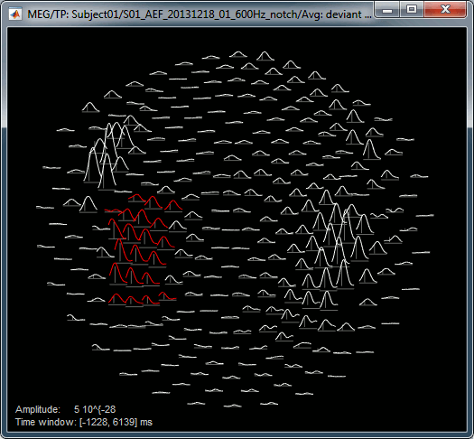
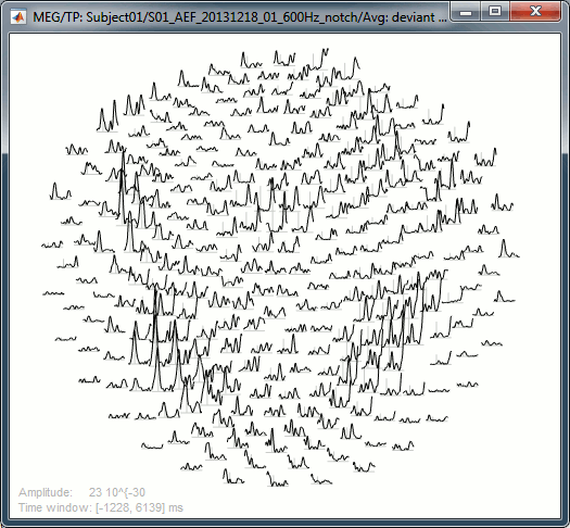
Useful shortcuts for these figures:
Left/right arrows: Change the current time.
Up/down arrows: Change the current frequency.
Control + E: Display the sensors markers/names.
Shift + click on a sensor: Displays the time-frequency decomposition for that specific sensors.
Right click + move: Select a group of sensors.
Shift + scroll: Change the gain of the time series (2D Layout).
Control + scroll: Change the length of the window displayed around the current time (2D Layout).
Scouts
Similar calculations can be done at the level of the sources, either on the full cortex surface or on a limited number of regions of interests. We will start with the latter as it is usually an easier approach.
Drag and drop all the deviant trials from both runs, select [Process sources].
Run process "Frequency > Time-frequency (Morlet wavelets)".
Select the option "Use scouts" and select all the scouts defined in the previous tutorial.
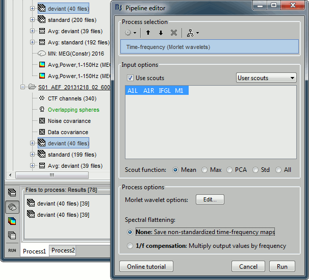
In the advanced options, select "Scout function: After" and "Output: Save average".
Run the process (it may take a while).
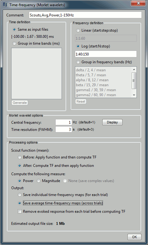
The scout function was introduced in the previous tutorial. It is the method we use to group the time series for the 20 dipoles we have in each scout into one unique signal. When computing the TF of one scout, we have the choice between applying this function before or after the time-frequency decomposition itself.
Before: Extract the 20 source signals, apply the scout function to get one signal, run the TF decomposition of this signal. This is faster but may lead to information loss.
After: Extract the 20 source signals, run the TF decomposition of the 20 signals, apply the scout function on the power of the TF maps. Always prefer this option when possible.
Rename the new file to add a tag "Deviant" in it. Then right-click > Time-freq: All scouts.
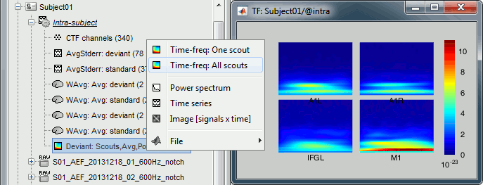
- In Process1, select the new average TF file.
Run process: Standardize > Baseline normalization, Baseline=[-75, 0]ms, Method=ERS/ERD.

Full cortical maps
Computing the time-frequency decomposition for all the sources of the cortex surface is possible but complicated because it can easily generate gigantic files, completely out of the reach of most computers. For instance the full TF matrix for each trial we have here would be [Nsources x Ntimes x Nfrequencies] = [15000 x 361 x 40] double-complex = 3.2 Gb!
We have two ways of going around this issue: computing the TF decomposition for fewer frequency bins or frequency bands at a time, or as we did previously, use only limited number of regions of interest.
In Process1, keep all the deviant trials both conditions selected, select [Process sources].
Run process "Frequency > Hilbert transform", No spectral flattening, Mirror signal before.
To process the entire brain, do not select the option "Use scouts".
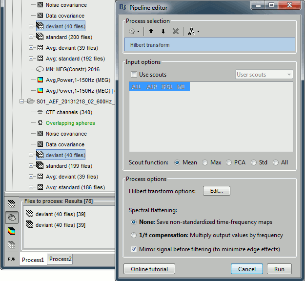
In the advanced options, select "Optimize storage: No", this option is not available when computing on the fly the average of multiple trials. Save the power, Save the average Hilbert maps.
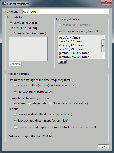
Optimize the storage of the time frequency file: Let's describe this option in more details.
- When computing the TF decomposition of a source file, we are actually applying sequentially two linear transformations to the original recordings: the TF analysis and the source inversion. These two processes can be permuted: TF(Inverse(Recordings)) = Inverse(TF(Recordings)).
Therefore we can optimize the TF computation time by applying the wavelet transformation only to the sensor recordings, and then multiply the wavelet complex coefficients by the inverse operator (ImagingKernel). This trick is always used in the computation of the Hilbert and Morlet transforms.
- When we have the option to the save the complex values (constrained sources and no averaging), this can also be used to optimize the storage of the files. In these cases, we save only the wavelet transformation of the sensor data. Later, when the file is loaded for display, the imaging kernel is applied on the fly. This can be disabled explicitly with this option.
- Rename the new Hilbert file to include the tag "Deviant", and select it in Process1.
Run process: Standardize > Baseline normalization, Baseline=[-75, 0]ms, Method=ERS/ERD.
Right-click on the Hilbert file > Display on cortex.
The frequency slider now shows frequency bands ("alpha:8-12Hz") instead of frequencies ("12Hz"). You can explore the source activity in time and frequency dimensions. The screen capture below shows the activity at 175ms: a 60% increase in the alpha band around the auditory cortex and a 20% decrease in the beta band around the motor cortex.

Shift + click on the cortex surface: Displays the TF decomposition of the selected source.
Right-click on the brain: Selects the closest vertex and displays the popup menu at the same time. The first three menus are relative to the source that was just clicked.
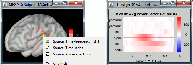
Unconstrained sources
In the current example, we are working with the simple case: sources with constrained orientations. The unconstrained case is more difficult to deal with, because we have to handle correctly the three orientations we have at each vertex.
Full cortex: Computes the TF decompositions for all the sources (3*15000=45000), then sum at each location the power for the three orientations.
Scouts: Option "Scout function" in the process.
Before: Extract the 20*3=60 source signals, apply the scout function to get three signals (one per orientation), run the TF decomposition of the three signals, and finally sum the power of the three TF maps. This is faster but may lose some frequency resolution (especially for constrained sources).
After: Extract the 20*3=60 source signals, run the TF decomposition of the 60 signals, apply the scout function on the power of the TF maps for each orientation separately, and finally sum the power obtained for the three orientations.
- The storage optimization option is not available with unconstrained sources.
Getting rid of the edge effects
To avoid making mistakes in the manipulation of the data and producing more readable figures, we encourage you to cut out the edge effects from your time frequency maps after computation.
- In Process1, select the very first computed in this tutorial: Test/Simulation/Power,1-60Hz | multiply
Run the process: "Extract > Extract time", Time window = [0.75, 5.25]s
Open the new file, select the option "Hide edge effects": Almost everything left in this new file is correctly estimated. Brainstorm keeps track of the edge effects in the TFmask field of the file.
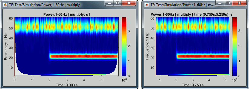
- We recommend you do the same when epoching your recordings: import trials that are longer than necessary, and after the time-frequency estimation, remove the unnecessary segments.
On the hard drive
Right click on the first TF file we computed > File > View file contents.
Structure of the time-frequency files: timefreq_*.mat
TF: [Nsignals x Ntime x Nfreq] matrix containing all the values of the time-frequency decomposition (complex wavelet coefficients, or double values for power/magnitude/Z-score).
TFmask: [Nfreq x Ntime] logical mask indicating the edge effects (0=edge, 1=valid value).
Std: [Nsignals x Ntime x Nfreq] standard deviation if this file is an average.
Comment: String displayed in the database explorer to represent the file.
DataType: From what kind of data this file was computed: {'data', 'results', 'scout, 'matrix'}
Time: [1 x Ntime] Time vector used to estimate this file.
TimeBands: [Ntimebands x 3] Cell array where each line represents a time band:
{'band_name', 'time definition', 'function'}Freqs: For regular frequency binning: vector containing all the frequencies.
If using frequency bands: [Nfreqbands x 3] cell array, where each line represents a frequency band {'band_name', 'frequency definition', 'function'}RefRowNames: Used only for connectivity matrices.
RowNames: [1 x Nsignals] Cell array of strings that describes each row of the TF matrix. In this specific case, it would be the list of all the MEG sensor names. But it could also be a list of names of scouts or clusters.
Measure: Contains the name of the function that was applied right after the computation of the wavelet coefficients. So it represents the type of data contained in the TF matrix. Possible values:
none: No measure applied, TF contains the complex wavelet coefficients.
power: Power for each frequency, ie. the square of the amplitude: abs(coefficients)2
magnitude: abs(coefficients)
log: 10 * log10( abs(coefficients)2)
phase: angle(coefficients)
Method: String that identifies the process that generated the file:
{'morlet', 'fft', 'psd', 'hilbert', 'corr', 'cohere', 'granger', 'plv'}DataFile: Initial file from which this file was computed. In the database explorer, the TF file will be shown as a child of this DataFile file.
SurfaceFile / GridLoc / GridAtlas: Source space that was used, only for source files.
Leff: Effective number of averages = Number of trials that were averaged to obtain this file.
ColormapType: String, force a specific colormap type to be used when displaying this file.
DisplayUnits: String, force to use specific units when displaying this file.
Options: Options that were selected in the time-frequency options window.
History: List of operations performed on this file (menu File > View file history).
Useful functions
in_bst_timefreq(TimefreqFile): Read a time-frequency file.
in_bst(FileName, TimeWindow): Read any Brainstorm file with the possibility to load only a specific part of the file. "TimeWindow" is an range of time values in seconds: [tStart, tStop].
bst_process('LoadInputFile', FileName, Target, TimeWindow): The most high-level function for reading data files. "Target" is a string with the list of sensor names or types to load.
morlet_transform(): Applies complex Morlet wavelet transform to the time series in input.
Additional documentation
Articles
Bertrand O, Tallon-Baudry C (2000)
Oscillatory gamma activity in humans: a possible role for object representation
Int J Psychophysiol, 38(3):211-23Bruns A (2004)
Fourier-, Hilbert- and wavelet-based signal analysis: are they really different approaches?
J Neurosci Methods, 137(2):321-32Le Van Quyen M, Foucher J, Lachaux J, Rodriguez E, Lutz A, Martinerie J, Varela FJ (2001)
Comparison of Hilbert transform and wavelet methods for the analysis of neuronal synchrony
J Neurosci Methods, 111(2):83-98Pantazis D, Weber DL, Dale CL, Nichols TE, Simpson GV, Leahy RM (2005)
Imaging of oscillatory behavior in event-related MEG studies (pdf)
in Proceedings of SPIE, Computational Imaging III, Vol. 5674, eds C. Bouman and E. MillerPfurtscheller G (1992)
Event-related synchronization (ERS): an electrophysiological correlate of cortical areas at rest
Electroencephalogr Clin Neurophysiol, 83(1):62-9Series of lectures by Mike X Cohen:
http://www.mikexcohen.com/lectures.htmlCassani, R. & Falk, T. H. (2018)
Spectrotemporal Modeling of Biomedical Signals: Theoretical Foundation and Applications. in Reference Module in Biomedical Sciences (Elsevier, 2018).
Forum discussions
Forum: Time and frequency resolution:
http://neuroimage.usc.edu/forums/showthread.php?1848
Tutorial 26: Statistics
Authors: Francois Tadel, Elizabeth Bock, Dimitrios Pantazis, Richard Leahy, Sylvain Baillet
In this auditory oddball experiment, we would like to test for the significant differences between the brain response to the deviant beeps and the standard beeps, time sample by time sample. Until now we have been computing measures of the brain activity in time or time-frequency domain. We were able to see clear effects or slight tendencies, but these observations were always dependent on an arbitrary amplitude threshold and the configuration of the colormap. With appropriate statistical tests, we can go beyond these empirical observations and assess what are the significant effects in a more formal way.
Contents
- Random variables
- Histograms
- Statistical inference
- Parametric Student's t-test
- Example 1: Parametric t-test on recordings
- Correction for multiple comparisons
- Nonparametric permutation tests
- Example 2: Permutation t-test
- FieldTrip implementation
- Example 3: Cluster-based correction
- Example 4: Parametric test on sources
- Directionality: Difference of absolute values
- Example 5: Parametric test on scouts
- Convert statistic results to regular files
- Example 6: Nonparametric test on time-frequency maps
- Export to SPM
- On the hard drive
- Additional documentation
Random variables
In most cases we are interested in comparing the brain signals recorded for two populations or two experimental conditions A and B.
A and B are two random variables for which we have a limited number of repeated measures: multiple trials in the case of a single subject study, or multiple subject averages in the case of a group analysis. To start with, we will consider that each time sample and each signal (source or sensor) is independent: a random variable represents the possible measures for one sensor/source at one specific time point.
A random variable can be described with its probability distribution: a function which indicates what are the chances to obtain one specific measure if we run the experiment. By repeating the same experiment many times, we can approximate this function with a discrete histogram of observed measures.
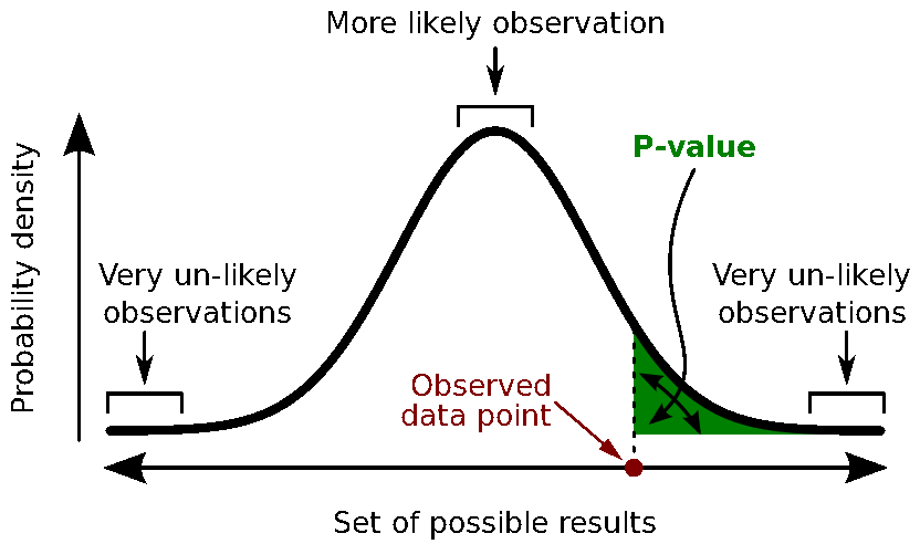
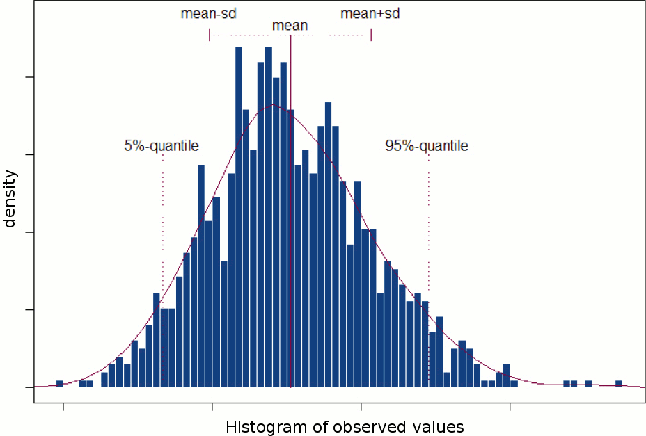
Histograms
You can plot histograms like this one in Brainstorm, it may help you understand what you can expect from the statistics functions described in the rest of this tutorial. For instance, seeing a histogram computed with only 4 values would discourage you forever from running a group analysis with 4 subjects...
Recordings
Let's evaluate the recordings we obtained for sensor MLP57, the channel that was showing the highest value at 160ms in the difference of averages computed in the previous tutorial.

We are going to extract only one value for each trial we have imported in the database, and save these values in two separate files, one for each condition (standard and deviant).
In order to observe more meaningful effects, we will process the trials together from the two acquisition runs. As explained in the previous tutorials (link), this is usually not recommended in MEG analysis, but it can be an acceptable approximation if the subject didn't move between runs.In Process1, select all the deviant trials from both runs.
Run process Extract > Extract values:
Options: Time=[160,160]ms, Sensor="MLP57", Concatenate time (dimension 2)
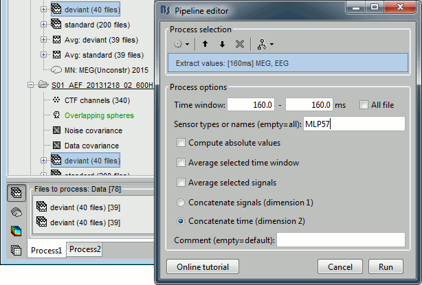
Repeat the same operation for all the standard trials.
You obtain two new files in the folder Intra-subject. If you look inside the files, you can observe that the size of the Value matrix matches the number of trials (78 for deviant, 383 for standard). The matrix is [1 x Ntrials] because we asked to concatenate the extracted values in the 2nd dimension.

To display the distribution of the values in these two files:
select them simultaneously, right-click > File > View histograms.
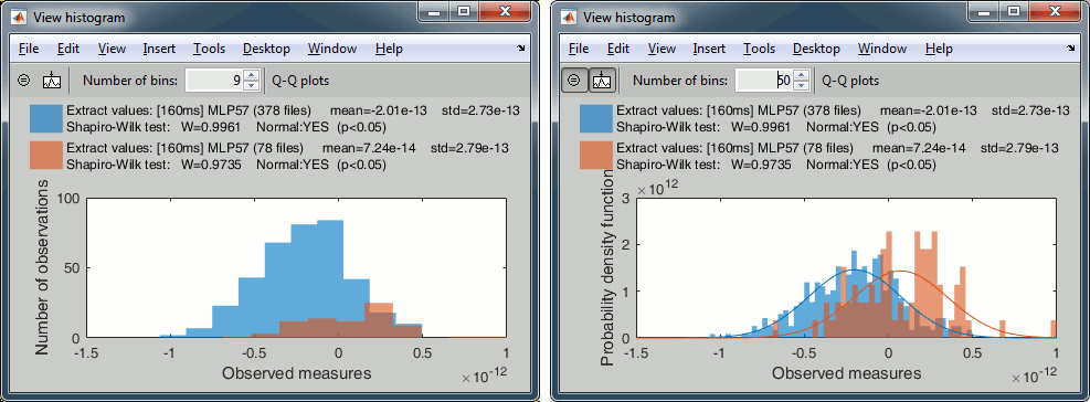
With the buttons in the toolbar, you can edit the way these distributions are represented: number of bins in the histogram, total number of occurrences (shows taller bars for standard because it has more values) or density of probability (normalized by the total number of values).
In addition, you can plot the normal distribution corresponding to the mean μ and standard deviation σ computed from the set of values (using Matlab functions mean and std).When comparing two sample sets A and B, we try to evaluate if the distributions of the measures are equal or not. In most of the questions we explore in EEG/MEG analysis, the distributions are overlapping a lot. The very sparse sampling of the data (a few tens or hundreds of repeated measures) doesn't help with the task. Some representations will be more convincing than others to estimate the differences between the two conditions.

The legend of the histograms shows the result of the Shapiro-Wilk normality test, as implemented by Ahmed BenSaïda (Matlab FileExchange). The button "Q-Q plots" gives another way to compare the current samples to the normal distribution (see: Wikipedia, Matlab FileExchange).
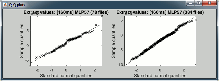
- Everything seems to indicate that the values recorded on the sensor MLP57 at 160ms follow a normal distribution, in both conditions.
Sources (relative)
We can repeat the same operation at the source level and extract all the values for scout A1L.
In Process1, select all the deviant trials from both runs. Select button [Process sources].
Run process Extract > Extract values: Time=[160,160]ms, Scout="A1L"
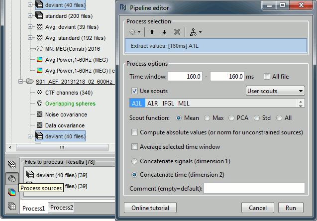
Repeat the same operation for all the standard trials.
Select the two files > Right-click > File > View histogram.
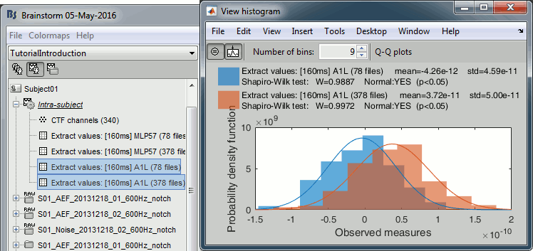
- The distributions still look normal, but the variances are now slightly different. You have to pay attention to this information when choosing which parametric t-test to run.
Sources (absolute)
Run again the process Extract > Extract values, but this time select Compute absolute values.
Display the histograms of the two rectified files.
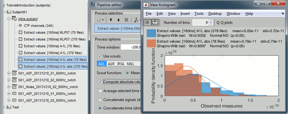
The rectified source values are definitely not following a normal distribution, the shape of the histogram has nothing to do with the corresponding Gaussian curves. As a consequence, if you are using rectified source maps, you will not be able to run independent parametric t-tests.
Additionally, you may have issues with the detection of some effects (see tutorial Difference).
Time-frequency
Time-frequency power for sensor MLP57 at 55ms / 48Hz (left=no normalization, right=ERS/ERD):

- These sample sets are clearly not normally distributed. Parametric t-tests don't look like good candidates for testing time-frequency power across trials.
Group studies and central limit theorem
The observations above hold only for the specific case we are looking at: single subject analysis, testing for differences across trials.
In the context of a group analysis, we usually test subject averages between conditions or populations. This corresponds to comparing the distributions of the mean of the trials across subjects, which will tend to be normal when we increase the number of trials (Central-limit theorem). In general, it is easier to obtain sample sets with normal distributions at the group level.
Additionally, some tricks can help bringing the samples closer to a normal distribution, like averaging in time/space/frequencies, or testing the square root of the data, in the case of time-frequency power. Some solutions are explored in (Kiebel, Tallon-Baudry & Friston, HBM 2005).
Statistical inference
Hypothesis testing
To show that there is a difference between A and B, we can use a statistical hypothesis test. We start by assuming that the two sets are identical then reject this hypothesis. For all the tests we will use here, the logic is similar:
Define a null hypothesis (H0:"A=B") and an alternative hypothesis (eg. H1:"A<B").
- Make some assumptions on the samples we have (eg. A and B are independent, A and B follow normal distributions, A and B have equal variances).
Decide which test is appropriate, and state the relevant test statistic T (eg. Student t-test).
Compute from the measures (Aobs, Bobs) the observed value of the test statistic (tobs).
Calculate the p-value. This is the probability, under the null hypothesis, of sampling a test statistic at least as extreme as that which was observed. A value of (p<0.05) for the null hypothesis has to be interpreted as follows: "If the null hypothesis is true, the chance that we find a test statistic as extreme or more extreme than the one observed is less than 5%".
Reject the null hypothesis if and only if the p-value is less than the significance level threshold (α).
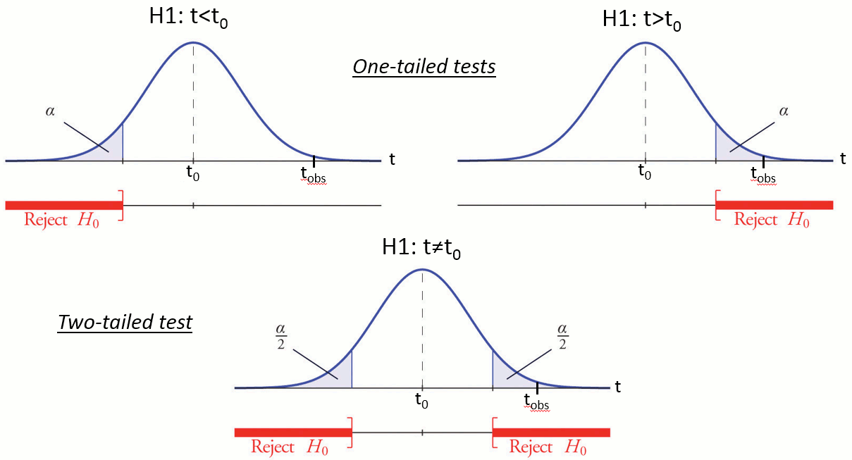
Evaluation of a test
The quality of test can be evaluated based on two criteria:
Sensitivity: True positive rate = power = ability to correctly reject the null hypothesis and control for the false negative rate (type II error rate). A very sensitive test detects a lot of significant effects, but with a lot of false positive.
Specificity: True negative rate = ability to correctly accept the null hypothesis and control for the false positive rate (type I error rate). A very specific test detects only the effects that are clearly non-ambiguous, but can be too conservative and miss a lot of the effects of interest.
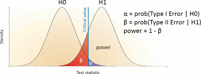
Different categories of tests
Two families of tests can be helpful in our case: parametric and nonparametric tests.
Parametric tests need some strong assumptions on the probability distributions of A and B then use some well-known properties of these distributions to compare them, based on a few simple parameters (typically the mean and variance). The estimation of these parameters is highly optimized and requires very little memory. The examples which will be described here are the Student's t-tests.
Nonparametric tests do not require any assumption on the distribution of the data. They are therefore more reliable and more generic. On the other hand, they are a lot more complicated to implement: they require a lot more memory because all the tested data has to be loaded at once, and a lot more computation time because the same test is repeated thousands of times.
Parametric Student's t-test
Assumptions
The Student's t-test is a widely-used parametric test to evaluate the difference between the means of two random variables (two-sample test), or between the mean of one variable and one known value (one-sample test). If the assumptions are correct, the t-statistic follows a Student's t-distribution.
The main assumption for using a t-test is that the random variables involved follow a normal distribution (mean: μ, standard deviation: σ). The figure below shows a few example of normal distributions.
t-statistic
Depending on the type of data we are testing, we can have different variants for this test:
One-sample t-test (testing against a known mean μ0):

where is the sample mean, σ is the sample standard deviation and n is the sample size.
 Dependent t-test for paired samples (eg. when testing two conditions across a group of subjects). Equivalent to testing the difference of the pairs of samples against zero with a one-sample t-test:

where D=A-B, is the average of D and σD its standard deviation.
 Independent two-sample test, equal variance (equal or unequal sample sizes):

where and
and  are the unbiased estimators of the variances of the two samples.
 Independent two-sample test, unequal variance (Welch's t-test):

where and
and  are the sample sizes of A and B.
p-value
Once the t-value is computed (tobs in the previous section), we can convert it to a p-value based on the known distributions of the t-statistic. This conversion depends on two factors: the number of degrees of freedom and the tails of the distribution we want to consider. For a two-tailed t-test, the two following commands in Matlab are equivalent and can convert the t-values in p-values.
p = betainc(df./(df + t.^2), df/2, 0.5);    % Without the Statistics toolbox
p = 2*(1 - tcdf(abs(t),df));                % With the Statistics toolbox
The distribution of this function for different numbers of degrees of freedom:
Example 1: Parametric t-test on recordings
Parametric t-tests require the values tested to follow a normal distribution. The recordings evaluated in the histograms sections above (MLP57/160ms) show distributions that are matching this assumption relatively well: the histograms follow the traces of the corresponding normal functions, and the two conditions have very similar variances. It looks reasonable to use a parametric t-test in this case.
In the Process2 tab, select the following files, from both runs (approximation discussed previously):
Files A: All the deviant trials, with the [Process recordings] button selected.
Files B: All the standard trials, with the [Process recordings] button selected.
The t-tests work well with unbalanced number of samples: It is better to use all the possible samples you have, even if you have 80 trials in one condition and 400 in the other.
Run the process "Test > Parametric test: Independent": Select all the data, do not average.
Sensor types: Leave this empty instead of entering "MEG", it won't affect the results but the computation will be faster (optimized when processing full files).
Test: Student's t-test (equal variance), two-tailed.
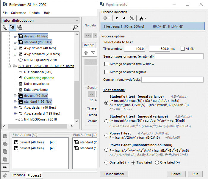
Double-click on the new file and add a 2D topography (CTRL+T). The values displayed in the 2D view are the significant t-values. All the sensors that have p-values higher than the significance level threshold (α) are set to zero.
With the new Stat tab you can control the significance level α and the correction you want to apply for multiple comparisons (see next section).
With the option minimum duration, you can exclude from the display all the data points that are significant only for isolated time samples, and which are mostly likely false positives. If this parameter is set to zero it has no impact on the display. Otherwise all the data points that are not significant continuously for at least this duration are set to zero.

Correction for multiple comparisons
Multiple comparison problem
The approach described in this first example performs many tests simultaneously. We test, independently, each MEG sensor and each time sample across the trials, so we run a total of 274*361 = 98914 t-tests.
If we select a critical value of 0.05 (p<0.05), it means that we want to see what is significantly different between the conditions while accepting the risk of observing a false positive in 5% of the cases. If we run the test around 100,000 times, we can expect to observe around 5,000 false positives. We need to better control for false positives (type I errors) when dealing with multiple tests.
Bonferroni correction
The probability to observe at least one false positive, or familywise error rate (FWER) is almost 1:
FWER = 1 - prob(no significant results) = 1 - (1 - 0.05)^100000 ~ 1
A classical way to control the familywise error rate is to replace the p-value threshold with a corrected value, to enforce the expected FWER. The Bonferroni correction sets the significance cut-off at  /Ntest. If we set (p ≤
  /Ntest), then we have (FWER ≤
  ). Following the previous example:
FWER = 1 - prob(no significant results) = 1 - (1 - 0.05/100000)^100000 ~ 0.0488 < 0.05
This works well in a context where all the tests are strictly independent. However, in the case of MEG/EEG recordings, the tests have an important level of dependence: two adjacent sensors or time samples often have similar values. In the case of highly correlated tests, the Bonferroni correction tends too be conservative, leading to a high rate of false negatives.
FDR correction
The false discovery rate (FDR) is another way of representing the rate of type I errors in null hypothesis testing when conducting multiple comparisons. It is designed to control the expected proportion of false positives, while the Bonferroni correction controls the probability to have at least one false positive. FDR-controlling procedures have greater power, at the cost of increased rates of Type I errors (Wikipedia)
In Brainstorm, we implement the Benjamini–Hochberg step-up procedure (1995):
Sort the p-values p(k) obtained across all the multiple tests (k=1..Ntest).
Find the largest k such as p(k) < k / Ntest *
 .
. Reject the null hypotheses corresponding to the first k smallest p-values.
This is is the same procedure as Matlab's call: mafdr(p, 'BHFDR', alpha)
Note that there are different implementations of FDR. FieldTrip uses the Benjamini–Yekutieli (2001) algorithm as described in (Genovese, 2002), which usually gives less true positive results. Don't be surprised if you get empty displays when using the option "FDR" in the FieldTrip processes, while you get significant results with the Brainstorm FDR correction.
In the interface
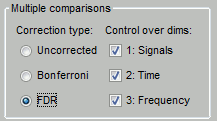
You can select interactively the type of correction to apply for multiple comparison while reviewing your statistical results. The checkboxes "Control over dims" allow you to select which are the dimensions that you consider as multiple comparisons (1=sensor, 2=time, 3=not applicable here). If you select all the dimensions, all the values available in the file are considered as the same repeated test, and only one corrected p-threshold is computed for all the time samples and all the sensors.
If you select only the first dimension, only the values recorded at the same time sample are considered as repeated tests, the different time points are corrected independently, with one different corrected p-threshold for each time point.
When changing these options, a message is displayed in the Matlab command window, showing the number of repeated tests that are considered, and the corrected p-value threshold (or the average if there are multiple corrected p-thresholds, when not all the dimensions are selected):
BST> Average corrected p-threshold: 5.0549e-07  (Bonferroni, Ntests=98914)
BST> Average corrected p-threshold: 0.00440939  (FDR, Ntests=98914)
"It doesn't work"
If nothing appears significant after correction, don't start by blaming the method ("FDR doesn't work"). In the first place, it's probably because there is no clear difference between your sample sets or simply because your sample size is too small. For instance, with less than 10 subjects you cannot expect to observe very significant effects in your data.
If you have good reasons to think your observations are meaningful but cannot increase the sample size, consider reducing the number of multiple comparisons you perform (test only the average over a short time window, a few sensors or a region of interest) or using a cluster-based approach. When using permutation tests, increasing the number of random permutations also decreases the p-value of the very significant effects.
Nonparametric permutation tests
Principle
A permutation test (or randomization test) is a type of test in which the distribution of the test statistic under the null hypothesis is obtained by calculating all possible values of the test statistic under rearrangements of the labels on the observed data points. (Wikipedia)
If the null hypothesis is true, the two sets of tested values A and B follow the same distribution. Therefore the values are exchangeable between the two sets: we can move one value from set A to set B, and one value from B to A, and we expect to obtain the same value for the test statistic T.
By taking all the possible permutations between sets A and B and computing the statistic for each of them, we can build a histogram that approximates the permutation distribution.
Then we compare the observed statistic with the permutation distribution. From the histogram, we calculate the proportion of permutations that resulted in a larger test statistic than the observed one. This proportion is called the p-value. If the p-value is smaller than the critical value (typically 0.05), we conclude that the data in the two experimental conditions are significantly different.
The number of possible permutations between the two sets of data is usually too large to compute an exhaustive permutation test in a reasonable amount of time. The permutation distribution of the statistic of interest is approximated using a Monte-Carlo approach. A relatively small number of random selection of possible permutations can give us a reasonably good idea of the distribution.
Permutation tests can be used for any test statistic, regardless of whether or not its distribution is known. The hypothesis is about the data itself, not about a specific parameter. In the examples below, we use the t-statistic, but we could use any other function.
Practical limitations
Computation time: If you increase the number of random permutations you use for estimating the distribution, the computation time will increase linearly. You need to find a good balance between the total computation time and the accuracy of the result.
Memory (RAM): The implementations of the permutation tests available in Brainstorm require all the data to be loaded in memory before starting the evaluation of the permutation statistics. Running this function on large datasets or on source data could quickly crash your computer. For example, loading the data for the nonparametric equivalent to the parametric t-test we ran previously would require:
276(sensors) * 461(trials) * 361(time) * 8(bytes) / 1024^3(Gb) = 0.3 Gb of memory.
This is acceptable on most recent computers. But to perform the same at the source level, you need:
45000*461*361*8/1024^3 = 58 Gb of memory just to load the data. This is impossible on most computers, we have to give up at least one dimension and run the test only for one region of interest or one time sample (or average over a short time window).
Example 2: Permutation t-test
Let's run the nonparametric equivalent to the test we ran in the first example.
In the Process2 tab, select the following files, from both runs (approximation discussed previously):
Files A: All the deviant trials, with the [Process recordings] button selected.
Files B: All the standard trials, with the [Process recordings] button selected.
Run the process "Test > Permutation test: Independent", set the options as shown below.
Sensor type: You should enter explicitly "MEG" instead of leaving this field empty. It will decrease the computation time (no optimization for full files in the nonparametric tests).
Note that it may require more than 3Gb of RAM and take more than 10min.
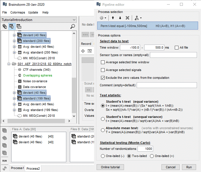
Open the parametric and nonparametric results side by side, the results should be very similar. You may have to increase the significance level α to 0.05 to see something significant in the nonparametric version (edit the value in the Stat tab). Alternatively, you can obtain lower p-values by running the same process with more randomizations (for instance 2000 or 10000).
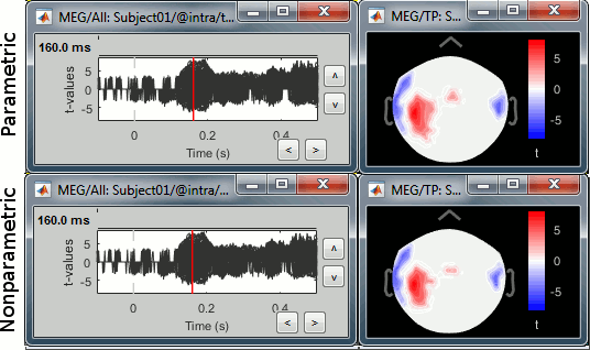
In this case, the distributions of the values for each sensor and each time point (non-rectified MEG recordings) are very close to normal distributions. This was illustrated at the top of this page, in the section "Histograms". Therefore the assumptions behind the parametric t-test are verified, the results of the parametric tests are correct and very similar to the nonparametric ones.
- If you get different results with the parametric and nonparametric approaches: trust the nonparametric one. If you want to increase the precision of a nonparametric test a decrease the p-values, increase the number of random permutations.
MacOS troubleshooting
Error "mexmaci64 cannot be opened because the developer cannot be verified":
FieldTrip implementation
FieldTrip functions in Brainstorm
We have the possibility to call some of the FieldTrip toolbox functions from the Brainstorm environment. If you are running the compiled version of Brainstorm these functions are already packaged with Brainstorm, otherwise you need to install FieldTrip on your computer, either manually or as a Brainstorm plugin. See the Plugins tutorial.
Cluster-based correction
One interesting method that has been promoted by the FieldTrip developers is the cluster-based approach for nonparametric tests. In the type of data we manipulate in MEG/EEG analysis, the neighboring channels, time points or frequency bins are expected to show similar behavior. We can group these neighbors into clusters to "accumulate the evidence". A cluster can have a multi-dimensional extent in space/time/frequency.
In the context of a nonparametric test, the test statistic computed at each permutation is the extent of the largest cluster. To reject or accept the null hypothesis, we compare the largest observed cluster with the randomization distribution of the largest clusters.
This approach solves the multiple comparisons problem, because the test statistic that is used (the maximum cluster size) is computed using all the values at the same time, along all the dimensions (time, sensors, frequency). There is only one test that is performed, so there is no multiple comparisons problem.
The result is simpler to report but also a lot less informative than FDR-corrected nonparametric tests. We have only one null hypothesis, "the two sets of data follow the same probability distribution", and the outcome of the test is to accept or reject this hypothesis. Therefore we cannot report the spatial or temporal extent of the most significant clusters. Make sure you read this recommendation before reporting cluster-based results in your publications.
Reference documentation
For a complete description of nonparametric cluster-based statistics in FieldTrip, read the following:
Article: Maris & Oostendveld (2007)
Video: Statistics using non-parametric randomization techniques (E Maris)
Video: Non-parametric cluster-based statistical testing of MEG/EEG data (R Oostenveld)
Tutorial: Parametric and non-parametric statistics on event-related fields
Tutorial: Cluster-based permutation tests on event related fields
Tutorial: Cluster-based permutation tests on time-frequency data
Tutorial: How NOT to interpret results from a cluster-based permutation test
Functions references: ft_timelockstatistics, ft_sourcestatistics, ft_freqstatistics
Process options
There are three separate processes in Brainstorm, to call the three FieldTrip functions.
ft_timelockstatistics: Compare imported trials (recordings).
ft_sourcestatistics: Compare source maps or time-frequency decompositions of sources.
ft_freqstatistics: Compare time-frequency decompositions of sensor recordings or scouts signals.
See below the correspondence between the options in the interface and the FieldTrip functions.
Test statistic options (name of the options in the interface in bold):
cfg.numrandomization = "Number of randomizations"
cfg.statistic = "Independent t-test" ('indepsamplesT') or "Paire t-test" ('depsamplesT)
cfg.tail = One-tailed (-1), Two-tailed (0), One-tailed (+1)
cfg.correctm = "Type of correction" ('no', 'cluster', 'bonferroni', 'fdr', 'max', 'holm', 'hochberg')
cfg.method = 'montecarlo'
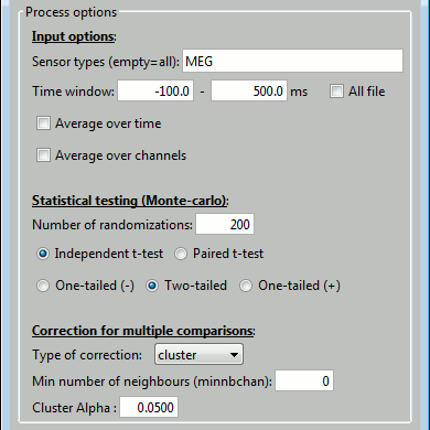
- cfg.correcttail = 'prob'
Cluster-based correction:
cfg.clusteralpha = "Cluster Alpha"
cfg.minnbchan = "Min number of neighours"
cfg.clustertail = cfg.tail (in not, FieldTrip crashes)
- cfg.clusterstatistic = 'maxsum'
Input options: All the data selection is done before, in the process code and functions out_fieldtrip_*.m.
- cfg.channel = 'all';
- cfg.latency = 'all';
- cfg.frequency = 'all';
- cfg.avgovertime = 'no';
- cfg.avgchan = 'no';
- cfg.avgoverfreq = 'no';
Example 3: Cluster-based correction
Run again the same test, but this time select the cluster correction.
- Keep the same files selected in Process2.
Run the process "Test > FieldTrip: ft_timelockstatistics", Type of correction = cluster
Note that it may require more than 5Gb of RAM and take more than 20min: check the Matlab command window for the FieldTrip progress report.
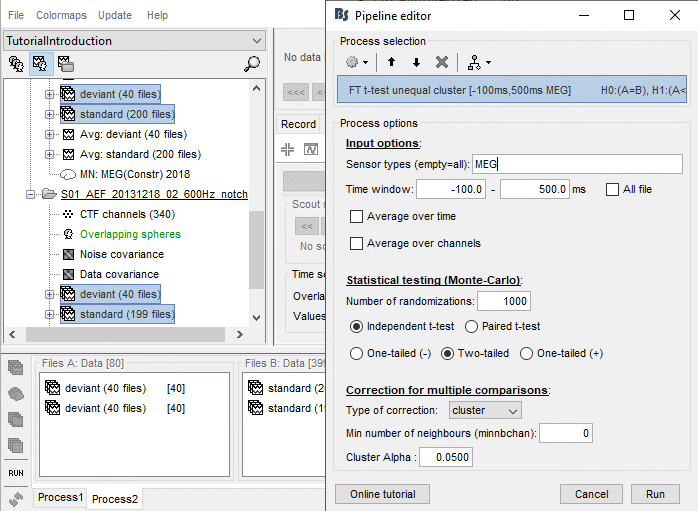
- Double-click on the new file, add a 2D topography to is (CTRL+T). Note that in the Stat tab, the options for multiple comparisons corrections are disabled, because the values saved in the file are already corrected, you can only change the significance threshold.
Instead, you get a list of significant clusters, which you can display separately if needed. The colored dots on the topography represent the clusters, blue for negative clusters and red for positive clusters. You can change these colors in the Stat tab. Note that the clusters have a spatio-temporal extent: at one time point they can be represented as two separate blobs in the 2D topography, but these blobs are connected at other time points.
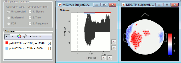
Additional options are available for exploring the clusters, try them all. Values used to represent the clusters: p=p-value, c=cluster statistic (maxsum), s=cluster size (connected data points).

Don't spend too much time exploring the clusters: In the previous cases, all the tests at each sensor and each time point were computed independently, we could report, individually, whether each of them was significant or not. On the other hand, the cluster-based approach just allows us to report that the two conditions are different, without specifying where or when, which makes the visual exploration of clusters relatively useless. Make sure you read this recommendation before reporting cluster-based results in your publications.
Example 4: Parametric test on sources
We can reproduce similar results at the source level. If you are using non-normalized and non-rectified current density maps, their distributions across trials should be normal, as illustrated earlier with the histograms. You can use a parametric t-test to compare the two conditions at the source level.
Keep the same files selected in Process2. Select the button [Process sources] on both sides.
Run the process "Test > Parametric test: Independent", Select all the data, do not average.
Use scouts: No. When this option is not selected, it uses the entire cortex instead.
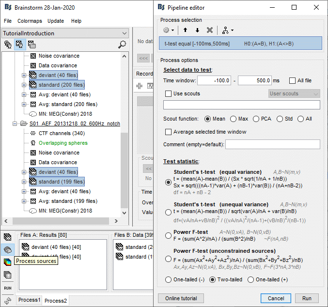
Double-click on the new file. Change the colormap definition to show only positive values (right-click > Colormap: Stat2 > Uncheck: Absolute values) and use a different colormap ("hot" or "jet"). The sign of the relative t-statistic is not meaningful, it depends mostly on the orientation of the dipoles on the cortex (see tutorial: Difference).

Scouts and statistics
From the Scout tab, you can also plot the scouts time series and get a summary of what is happening in your regions of interest. Non-zero values indicate the latencies when at least one vertex of the scout has a value that is significantly different between the two conditions. The values that are shown are the averaged t-values in the scout. The figure below shows the option "Values: Relative" to match surface display, but absolute values would make more sense in this case.

Unconstrained sources
There are some additional constraints to take into consideration when computing statistics for source models with unconstrained orientations. See the corresponding section in the tutorial Workflows.
Directionality: Difference of absolute values
The test we just computed detects correctly the time and brain regions with significant differences between the two conditions, but the sign of the t statistic is useless, we don't know where the response is stronger or weaker for the deviant stimulation.
After identifying where and when the responses are different, we can go back to the source values and compute another measure that will give us the directionality of this difference:
abs(average(deviant_trials)) - abs(average(standard_trials))
Keep the same files selected in Process2. Select the button [Process sources] on both sides.
Run process "Test > Difference of means", with the option "Absolute value of average".
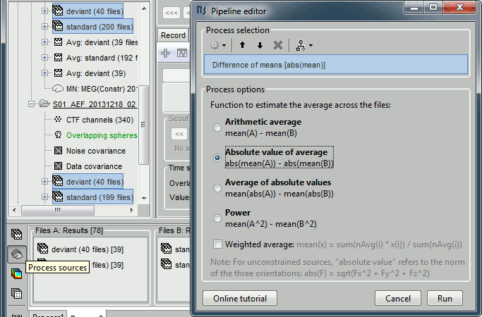
Double-click on the new file. Double-click on the colorbar to reset it to its defaults. The sign of this difference is meaningful: red values mean "higher amplitude for the deviant condition", blue values mean "higher amplitude for the standard condition", but we don't know if they are statistically significant.

The example above shows the two files at 148ms. The left figure shows the result of the t-test (significant effects but ambiguous sign) and the right figure shows the difference of absolute values (meaningful sign, but no statistical threshold). The superposition of the two information shows that there is some significant increase of activity in the frontal region for the deviant condition, but a decrease around the auditory cortex. This can be combined more formally as explained below.
- In Process2: FilesA = t-test results (sources), FilesB = difference deviant-standard (sources).
Run process: Test > Apply statistic threshold, significance level α=0.01, correction=FDR.
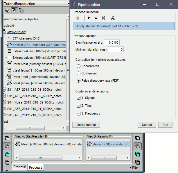
Double-click on the new file, go to 148ms. The statistic threshold from the t-test file was applied to the difference of rectified averages (deviant-standard): only the values for which there is a significant effect between the two conditions are kept, all the others are set to zero and masked. We observe areas colored in white where the two conditions have equal amplitudes but different signs. Note that for displaying this file correctly, you must keep the amplitude slider at 0% (in the Surface tab): a correct statistic threshold is already applied to the source map, you should not perform any additional random amplitude threshold on it.

Example 5: Parametric test on scouts
The previous example showed how to test for differences across the full source maps, and then to extract the significant scout activity. Another valid approach is to test directly for significant differences in specific regions of interest, after computing the scouts time series for each trial.
This alternative has many advantages: it can be a lot faster and memory-efficient and it reduces the multiple comparisons problem. Indeed, when you perform less tests at each time point (the number of scouts instead of the number of sources), the FDR and Bonferroni corrections are less conservative and lead to higher p-values. On the other hand, it requires to formulate stronger hypotheses: you need to define the regions in which you expect to observe differences, instead of screening the entire brain.
In Process2, select all the deviant trials (A) and standard trials (B). Select [Process sources].
Run process Test > Parametric test: Independent, Use scouts: A1L, IFGL, M1L.
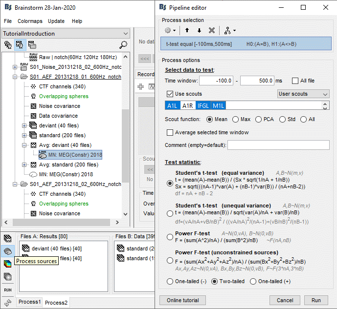
Double-click on the new file. It shows the time points where the scout signals (averaged across vertices) are significantly different in the two conditions. We cannot represent this new file over the cortex because we have restricted the test to the scouts and discarded all the spatial information. As explained in the previous examples: the significant differences are correctly detected but the sign of the t-statistic is ambiguous.

Convert statistic results to regular files
Apply statistic threshold
You can convert the results of a statistic test to a regular file. It can be useful because lots of menus and processes are not accessible for the files with the "stat" tag display on top of their icon.
- In Process1: Select the results for the test you ran on scouts time series (example #5).
Run process: "Test > Apply statistic threshold": α=0.01, correction=FDR, dim=[all].
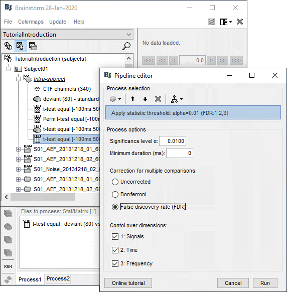
- It produces a new file with the same name but without the "stat" tag. This file is a regular matrix that you can use with any process. When you open it, the Stat tab doesn't show up.
Note that when using this process from the Process1 tab, with one single stat file in input, the values saved in the file are the t-values from the stat file, not the original physical units. In order to obtain real physical units, you need to call the process with two inputs: the stat file on the left, and the file with the values of interest on the right, as in the previous section Directionality: Difference of absolute values.
Simulate recordings from these scouts
Compute a head model for the intra-subject folder:
Right-click on the channel file > Compute head model, keep all the default options.
Note that this channel file was created during one of the processes involving the two runs, it contains an average of their respective channel files (average head positions).- In Process1, select the new thresholded matrix file.
Run process: "Simulate > Simulate recordings from scout", select option Save full sources.
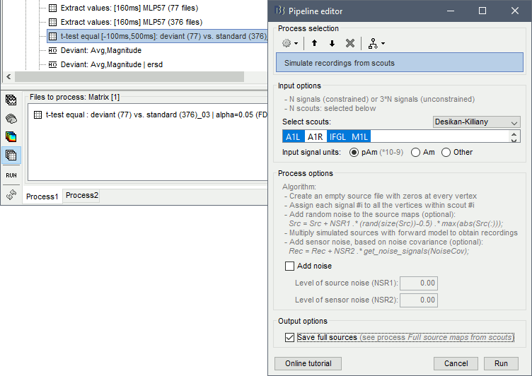
This process creates two files. First it maps the scouts time series on the cortex: it creates an empty source file with zeroes everywhere, then for each scout it maps the values of the input time times series to the sources within the ROI. Then it multiplies these artificial source maps with the forward model to simulate MEG recordings.

Note that this example is not adapted to simulate realistic MEG values. The source time series used in input for the process "Simulate recordings from scouts" are t-values, and not realistic physical units for a current source density (in pAm). The simulated MEG values localize correctly the simulated scouts, but with meaningless amplitudes. For realistic simulations, you must use input signals with amplitudes that correspond to minimum norm current density maps (in pAm). You can obtain these e.g. by computing them with process "Extract > Scout time series".
Example 6: Nonparametric test on time-frequency maps
Two run a test on time-frequency maps, we need to have all the time-frequency decompositions for each individual trial available in the database. In the time-frequency tutorial, we saved only the averaged time-frequency decompositions of all the trials.
In Process1, select all the trials from both conditions and both runs.
Run process "Frequency > Time-frequency (Morlet wavelets)". Select the options as below.
Select only one sensor (eg. MLP57) to make it faster. Save individual TF maps.
Measure=Magnitude: It is more standard to test the square root of power (amplitude).
Do not normalize the TF maps for a test within a single subject (only for group studies).
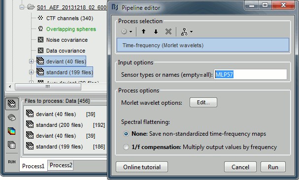
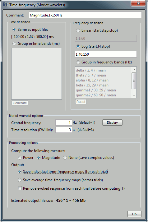
In Process2, select all the deviant trials (A) and standard trials (B). Select [Process time-freq].
Run process: Test > Permutation test: Independent, 1000 randomizations, no correction.
No need to select the option "Match signals between files" because the list of signals is the same for all the trials. If you have marked bad channels in some trials during your analysis, you would need to select this option.
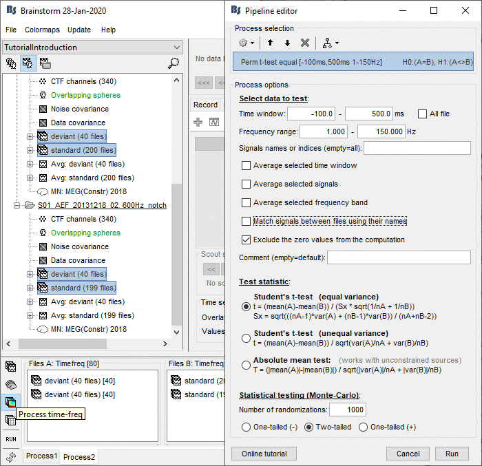
Double-click on the new file. In the Stat tab, select α=0.05 uncorrected.

If you run this test on time-frequency files where the power has been saved, you get this warning:

Now delete the TF decompositions for the individual trials:
- In Process1, select the files for which you computed the TF decomposition (all trials).
Select the [Process time-freq] button.
Run process: File > Delete files, option Delete selected files.
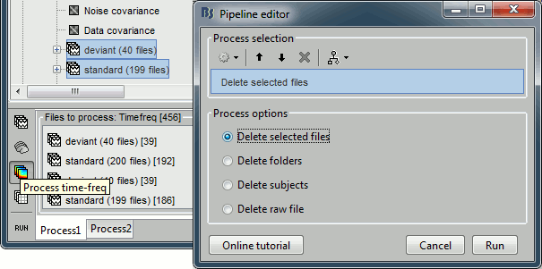
Export to SPM
An alternative to running the statistical tests in Brainstorm is to export all the data and compute the tests with an external program (R, Matlab, SPM, etc). Multiple menus exist to export files to external file formats (right-click on a file > File > Export to file).
Two tutorials explain how to export data specifically to SPM:
Export source maps to SPM8 (volume)
Export source maps to SPM12 (surface)
On the hard drive
Right click on the first test we computed in this tutorial > File > View file contents.
Description of the fields
pmap: [Nsignals x Ntime x Nfreq]: p-values for all the data points. If empty, computed from tmap:
pmap = process_test_parametric2('ComputePvalues', tmap, df, TestType, TestTail);tmap: [Nsignals x Ntime x Nfreq]: t-values for all the data points.
df: [Nsignals x Ntime x Nfreq]: Number of degrees of freedom for each test.
Correction: Correction for multiple comparison already applied ('no', 'cluster', 'fdr', ...)
Type: Initial type of the data ('data', 'results', 'timefreq', 'matrix').
Comment: String displayed in the database explorer to represent the file.
- The other fields were copied from the files that were tested, and were described previously.
Useful functions
process_test_parametric2: Two-sample independent parametric t-test
process_test_parametric2p: Two-sample paired parametric t-test
process_test_parametric1: One-sample parametric t-test (against zero)
process_ttest_baseline: One-sample parametric t-test (against baseline)
process_ft_timelockstatistics: FieldTrip tests for recordings (file type "data")
process_ft_sourcestatistics: FieldTrip tests for source maps (file type "results")
process_ft_freqstatistics: For time-frequency and scouts (file type "timefreq" and "matrix")
Conversion Brainstorm to FieldTrip: out_fieldtrip_data, out_fieldtrip_results, out_fieldtrip_timefreq, out_fieldtrip_matrix
process_extract_pthresh: Computes the pmap from the tmap, and saves thresholded files.
process_test_parametric2('ComputePvalues', t, df, TestType, TestTail)
bst_stat_thresh: Computes the Bonferroni and FDR corrections in Brainstorm.
Additional documentation
Articles
Bennett CM, Wolford GL, Miller MB, The principled control of false positives in neuroimaging
Soc Cogn Affect Neurosci (2009), 4(4):417-422.Maris E, Oostendveld R, Nonparametric statistical testing of EEG- and MEG-data
J Neurosci Methods (2007), 164(1):177-90.Maris E, Statistical testing in electrophysiological studies
Psychophysiology (2012), 49(4):549-65Bennett CM, Wolford GL, Miller MB, The principled control of false positives in neuroimaging
Soc Cogn Affect Neurosci (2009), 4(4):417-422.Pantazis D, Nichols TE, Baillet S, Leahy RM. A comparison of random field theory and permutation methods for the statistical analysis of MEG data, Neuroimage (2005), 25(2):383-94.
Kiebel SJ, Tallon-Baudry C, Friston K
Parametric analysis of oscillatory activity as measured with EEG/MEG, HBM 2005FieldTrip video: Non-parametric cluster-based statistical testing of MEG/EEG data:
https://www.youtube.com/watch?v=vOSfabsDUNg
Related tutorials
Forum discussions
Multiple comparisons: http://neuroimage.usc.edu/forums/showthread.php?1297
Cluster neighborhoods: http://neuroimage.usc.edu/forums/showthread.php?2132
Differences FieldTrip-Brainstorm: http://neuroimage.usc.edu/forums/showthread.php?2164
Statistics on sources: https://neuroimage.usc.edu/forums/t/11876
Citing the non-parametric tests in an article: https://neuroimage.usc.edu/forums/t/non-parametric-or-parametric-stats-implemented-in-brainstorm/24907/5
Conjunction inference: https://neuroimage.usc.edu/forums/t/common-source-activation-across-subjects-and-conditions/1152
Normalize PSD based on resting-state before statistical tests: https://neuroimage.usc.edu/forums/t/psd-normalization-based-on-the-resting-psd/37854
Tutorial 27: Workflows
Authors: Francois Tadel, Elizabeth Bock, Dimitrios Pantazis, John Mosher, Richard Leahy, Sylvain Baillet
This page provides some general recommendations for your event-related analysis. It is not directly related with the auditory dataset, but provides guidelines you should consider for any MEG/EEG experiment.
We do not provide standard analysis pipelines for resting or steady state recordings yet, but we will add a few examples soon in the section Other analysis scenarios of the tutorials page.
Contents
What is your question?
The most appropriate analysis pipeline for your data depends on the question you are trying to answer. Before defining what are the main steps of your analysis, you should be able to state clearly the question you want to answer with your recordings.
What dimension?
- MEG/EEG recordings
- Cortical sources
- Individual anatomy or template
- Constrained (one value per vertex) or unconstrained (three values per grid point)
- Full cortex or regions of interests
- Frequency or time-frequency maps
What kind of experiment?
Single subject: Contrast two experimental conditions across trials, for one single subject.
- Files A: Single trials for condition A.
- Files B: Single trials for condition B.
Group analysis, within subject: Contrast two conditions A and B measured for each subject.
- Files A: Subject-level averages for condition A (all the subjects).
- Files B: Subject-level averages for condition B (all the subjects).
Group analysis, between subjects: Contrast two groups of subjects for one condition.
- Files A: Subject-level averages for group #1 (G1).
- Files B: Subject-level averages for group #2 (G2).
What level of precision?
- Difference of averages
- Statistically significant differences between conditions or groups
What statistical test?
A = B
Tests the null hypothesis H0:(A=B) against the alternative hypothesis H1:(A≠B)
Correct detection: Identify correctly where and when the conditions are different.
- Ambiguous sign: We cannot say which condition is stronger.
Power(A) = Power(B)
Tests the null hypothesis H0:(Power(A)=Power(B)) against the alternative hypothesis H1:(Power(A)≠Power(B))
- Incorrect detection: Not sensitive to the cases where A and B have opposite signs.
Meaningful sign: We can identify correctly which condition has a stronger response.
Power(x) = |x|2, where |x| represents the modulus of the values:
- Absolute value for scalar values (recordings, constrained sources, time-frequency)
- Norm of the three orientations for unconstrained sources.
Multiple comparisons: FDR is a good choice for correcting p-values for multiple comparisons.
Design considerations
- Use within-subject designs whenever possible (i.e. collect two conditions A and B for each subject), then contrast data at the subject level before comparing data between subjects.
- Such designs are not only statistically optimal, but also ameliorate the between-subject sign ambiguities as contrasts can be constructed within each subject.
Common pre-processing pipeline
Most event-related studies can start with the pipeline we've introduced in these tutorials.
- Import the anatomy of the subject (or use a template for all the subjects).
- Access the recordings:
- Link the continuous recordings to the Brainstorm database.
- Prepare the channel file: co-register sensors and MRI, edit type and name of channels.
- Edit the event markers: fix the delays of the triggers, mark additional events.
- Pre-process the signals:
- Evaluate the quality of the recordings with a power spectral density plot (PSD).
- Apply frequency filters (low-pass, high-pass, notch).
- Identify bad channels and bad segments.
- Correct for artifacts with SSP or ICA.
- Import the recordings in the database: epochs around some markers of interest.
How many trials to include?
Single subject: Include all the good trials (unless you have a very low number of trials).
See the averaging tutorial.Group analysis: Use a similar numbers of trials for all the subjects (no need to be strictly equal), reject the subjects for which you have much less good trials.
EEG recordings
Average
- Average the epochs across acquisition runs: OK.
- Average the epochs across subjects: OK.
- Electrodes are in the same standard positions for all the subjects (e.g. 10-20).
- Never use an absolute value for averaging or contrasting sensor-level data.
Statistics: Single subject
A = B: Parametric or non-parametric t-test, independent, two-tailed.
Statistics: Group analysis, within subject
A = B
First-level statistic: For each subject, sensor average for conditions A and B.
Second-level statistic: Parametric or non-parametric t-test, paired, two-tailed.
Statistics: Group analysis, between subjects
G1 = G2
First-level statistic: For each subject, sensor average for the conditions to test.
Second-level statistic: Parametric/non-parametric t-test, independent, two-tailed.
MEG recordings
Average
- Average the epochs within each acquisition runs: OK.
- Average across runs: Not advised because the head of the subject may move between runs.
- Average across subjects: Strongly discouraged because the shape of the heads vary but the sensors are fixed. One sensor does not correspond to the same brain region for different subjects.
- Tolerance for data exploration: Averaging across runs and subjects can be useful for identifying time points and sensors with interesting effects but should be avoided for formal analysis.
- Note for Elekta/MaxFilter users: You can align all acquisition run to a reference run, this will allow direct channel comparisons and averaging across runs. Not recommended across subjects.
- Never use an absolute value for averaging or contrasting sensor-level data.
Statistics: Single subject
A = B: Parametric or non-parametric t-test, independent, two-tailed.
Statistics: Group analysis
- Not recommended with MEG recordings: do your analysis in source space.
Constrained cortical sources
Average: Single subject
Sensor average: Compute one sensor-level average per acquisition run and per condition.
Sources: Estimate sources for each average (constrained, no normalization).
Source average: Average the source-level run averages to get one subject average.
Compute a weighted average to balance for different numbers of trials across runs.Low-pass filter your evoked responses (optional).
If you filter the average before normalizing wrt baseline, it will lead to an underestimation of the baseline variance, and therefore to an overestimation of the Z scores computed in the next step, especially if the baseline is too short (typically less than 200 time points). The filter increases the autocorrelation of the time series, and therefore biases the estimation of the signal variance (Wikipedia).
You have to take into account the possible edge effects due to the filter. You can either extract a small time window or exclude the beginning of the baseline for the normalization.
Normalize the subject min-norm averages: Z-score wrt baseline (no absolute value).
Justification: The amplitude range of current densities may vary between subjects because of anatomical or experimental differences. This normalization helps bringing the different subjects to the same range of values.Do not rectify the cortical maps, but display them as absolute values if needed.
Average: Group analysis
Subject averages: Compute within-subject averages for all the subjects, as described above.
Rectify the cortical maps (process: Pre-process > Absolute value).
Justification: Cortical maps have ambiguous signs across subjects: reconstructed sources depend heavily on the orientation of true cortical sources. Given the folding patterns of individual cortical anatomies vary considerably, cortical maps have subject-specific amplitude and sign ambiguities. This is true even if a standard anatomy is used for reconstruction.Project the individual source maps on a template (only when using the individual brains).
For more details, see tutorial: Group analysis: Subject coregistration.Group average: Compute grand averages of all the subjects.
Do not use a weighted average: all the subjects should have the same weight in this average.Smooth spatially the source maps (optional).
You can smooth after step #3 for computing non-parametric statistics with the subject averages. For a simple group average, it is equivalent to smooth before of after computing the average.
Difference of averages: Within subject
Sensor average: Compute one sensor-level average per acquisition run and condition.
Sources: Estimate sources for each average (constrained, no normalization).
Source average: Average the source-level session averages to get one subject average.
Subject difference: Compute the difference between conditions for each subject #i: (Ai-Bi)
Low-pass filter the difference (optional)
Normalize the difference: Z-score wrt baseline (no absolute value): Z(Ai-Bi)
Rectify the difference (apply an absolute value): |Z(Ai-Bi)|
Project the individual difference on a template (only when using the individual brains).
Group average: Compute grand averages of all the subjects: avg(|Z(Ai-Bi)|).
Smooth spatially the source maps (optional).
Difference of averages: Between subjects
Grand averages: Compute averages for groups #1 and #2 as in Average:Group analysis.
Difference: Compute the difference between group-level averages: avg(|G1|)-avg(|G2|)
Limitations: Because we rectify the source maps before computing the difference, we lose the ability to detect the differences between equal values of opposite signs. And we cannot keep the sign because we are averaging across subjects. Therefore, many effects are not detected correctly.
Statistics: Single subject
A = B: Parametric or non-parametric
- Compute source maps for each trial (constrained, no normalization).
Parametric or non-parametric two-sample t-test, independent, two-tailed.
Identifies correctly where and when the conditions are different (sign not meaningful).Directionality: Additional step to know which condition has higher values.
Compute the difference of rectified averages: |avg(Ai)|-|avg(Bi)|
Combine the significance level (t-test) with the direction (difference): See details.
|mean(A)| = |mean(B)|: Non-parametric
- Compute source maps for each trial (constrained, no normalization).
Non-parametric independent two-sample "absolute mean test", two-tailed.
T = (|mean(A)|-|mean(B)|) / sqrt(|var(A)|/NA + |var(B)|/NB)- Interesting alternative that provides at the time a correct estimation of the difference (where and when) and the direction (which condition has higher values).
Statistics: Group analysis, within subject
Power(A-B) = 0: Parametric
First-level statistic: Rectified difference of normalized averages.
Proceed as in Difference of averages: Within subjects, but stop before the group average (after step #8). You obtain one measure |Ai-Bi| per subject, test these values against zero.Second-level statistic: Parametric one-sample Chi2-test.
Power = sum(|Ai-Bi|2), i=1..Nsubj ~ Chi2(Nsubj)Identifies where and when the conditions are different (sign not meaningful).
- Warning: Very sensitive test, with lots of false positive (all the brain can be "significant")
|A| = |B|: Parametric or non-parametric
First-level statistic: Rectified and normalized subject averages.
Proceed as in Average: Group analysis to obtain two averages per subject: Ai and Bi.Second-level statistic: Parametric or non-parametric two-sample t-test, paired, two-tailed.
This test does not consider the sign difference within a subject, and therefore cannot detect correctly when A and B have opposite signs. Works well and indicates which condition has higher values when A and B have the same sign within a subject.
A = B: Parametric or non-parametric [anatomy template only]
First-level statistic: Normalized subject averages (not rectified, no projection needed).
Proceed as in Average: Single subject to obtain two averages per subject: Ai and Bi.Second-level statistic: Parametric or non-parametric two-sample t-test, paired, two-tailed.
Applies only if all the subjects are sharing the same template anatomy.
Not recommended when using individual anatomies because of the sign issue between subjects (the signs might be opposed between two subjects, and the projection of non-rectified values to a template might be inaccurate).
Power(A) = 0: Parametric
First-level statistic: Rectified and normalized subject averages.
Proceed as in Average: Group analysis to obtain one average per subject #i: |Ai|.Second-level statistic: Parametric one-sample Chi2-test.
PowerA = sum(|Ai|2), i=1..Nsubj ~ Chi2(Nsubj).
Statistics: Group analysis, between subjects
|G1| = |G2|: Non-parametric
First-level statistic: Rectified and normalized subject averages.
Proceed as in Average: Group analysis to obtain one average per subject.Second-level statistic: Non-parametric two-sample t-test, independent, two-tailed.
Power(G1) = Power(G2): Parametric
First-level statistic: Rectified and normalized subject averages.
Proceed as in Average: Group analysis to obtain one average per subject: |Ai|.Second-level statistic: Parametric two-sample power F-test.
PowerG1 = sum(Ai2), i=1..N1 ~ Chi2(N1)
PowerG2 = sum(Aj2), j=1..N2 ~ Chi2(N2)
F(N1,N2) = (PowerG1 / N1) / (PowerG2 / N2)
Unconstrained cortical sources
Three values for each grid point, corresponding to the three dipoles orientations (X,Y,Z).
We want only one statistic and one p-value per grid point in output.
Averages
- Proceed as indicated above for constrained cortical sources.
Just replace the step Rectify with Flatten (process: Sources > Unconstrained to flat map).
The operator |A| has to be interpreted as "norm of the three orientations":
|A| = sqrt(Ax2 + Ay2 + Az2)
Statistics: Single subject
|mean(A)| = |mean(B)|: Non-parametric
- Compute source maps for each trial (unconstrained, no normalization).
Non-parametric independent two-sample "absolute mean test", independent, two-tailed.
T = (|mean(A)|-|mean(B)|) / sqrt(|var(A)|/NA + |var(B)|/NB)- Provides at the time a correct estimation of the difference (where and when) and the direction (which condition has higher values).
Statistics: Group analysis, within subject
Power(A-B) = 0: Parametric
First-level statistic: Flattened difference of normalized averages.
Proceed as in Difference of averages: Within subjects, but stop before the group average (after step #8). You obtain one measure |Ai-Bi| per subject, test these values against zero.Second-level statistic: Parametric one-sample Chi2-test for unconstrained sources.
Power = sum(|Ai-Bi|2), i=1..Nsubj ~ Chi2(3*Nsubj)Identifies where and when the conditions are different (sign not meaningful).
- Warning: Very sensitive test, with lots of false positive (all the brain can be "significant")
|A| = |B|: Parametric or non-parametric
First-level statistic: Flattened and normalized subject averages.
Proceed as in Average: Group analysis to obtain two averages per subject: Ai and Bi.Second-level statistic: Parametric or non-parametric two-sample t-test, paired, two-tailed.
This test does not consider the sign difference within a subject, and therefore cannot detect correctly when A and B have opposite signs. Works well and indicates which condition has higher values when A and B have the same sign within a subject.
Power(A) = 0: Parametric
First-level statistic: Flattened and normalized subject averages.
Proceed as in Average: Group analysis to obtain one average per subject #i: |Ai|.Second-level statistic: Parametric one-sample Chi2-test for unconstrained sources.
PowerA = sum(|Ai|2) = sum(Aix2+Aiy2+Aiz2), i=1..Nsubj ~ Chi2(3*Nsubj).
Statistics: Group analysis, between subjects
|G1| = |G2|: Non-parametric
First-level statistic: Flattened and normalized subject averages.
Proceed as in Average: Group analysis to obtain one average per subject.Second-level statistic: Non-parametric two-sample t-test, independent, two-tailed.
Power(G1) = Power(G2): Parametric
First-level statistic: Flattened and normalized subject averages.
Proceed as in Average: Group analysis to obtain one average per subject: |Ai|.Second-level statistic: Parametric two-sample power F-test (unconstrained sources).
PowerG1 = sum(Aix2+Aiy2+Aiz2), i=1..N1 ~ Chi2(3*N1)
PowerG2 = sum(Ajx2+Ajy2+Ajz2), j=1..N2 ~ Chi2(3*N2)
F = (PowerG1 / N1) / (PowerG2 / N2) ~ F(3*N1,3*N2)
Regions of interest (scouts)
Statistics: Single subject
- Even within-subject cortical maps have sign ambiguities. MEG/EEG source mapping has limited spatial resolution and sources in opposing sulcal/gyral areas are typically reconstructed with inverted signs (constrained orientations only). Averaging activity in cortical regions of interest (scouts) would thus lead to signal cancelation. To mitigate this issue, Brainstorm uses algorithms to change the polarity of individual source time series before averaging across a scout cortical region. Please note however that the polarity of the resulting time series remains ambiguous, as it is determined by statistical considerations, not by physiological information.
We therefore recommend that you perform subject-wise averaging/contrast before averaging scout time series. You may also consider aggregating scout source time series using PCA instead of averaging, across all files (all epochs and conditions) from a subject together, ensuring the same component is applied everywhere and therefore mitigating further some of the ambiguities concerning the polarity of the source time series.
Statistics: Group analysis, within subject
- Comparison of scout time series between subjects is tricky because there is no way to avoid sign ambiguity for different subjects. Thus there are no clear recommendations. Rectifying before comparing scout time series between subjects can be a good idea or not depending on different cases.
- Having a good understanding of the data (multiple inspections across channels/sources/subjects) can offer hints whether rectifying the scout time series is a good idea. Using unconstrained cortical maps to create the scout time series can ameliorate ambiguity concerns.
Time-frequency maps
Average: Single subject
Single trials: Compute time-frequency maps for each trial (magnitude, no normalization).
It is a more standard analysis to take the square root of power before a t-test.Subject average: Average the time-frequency maps together, separately for each condition. This can be done automatically when computing the TF decompositions (option "Save averaged time-frequency maps" in the process options).
- The values are all strictly positive, there is no sign ambiguity: you can directly subtract the averages of the two conditions and interpret the sign of the difference.
- If you average time-frequency maps computed on sensor-level data, the same limitations apply as for averaging sensor level data (see sections about MEG and EEG recordings above).
Average: Group analysis
Subject averages: Compute within-subject averages for all the subjects, as described above.
Normalize the subject averages: ERD/ERS or Z-score wrt baseline.
Group average: Compute grand averages of all the subjects.
Difference of averages: Simply compute the difference of the group averages.
Statistics: Single subject
A = B: Parametric or non-parametric
Compute time-frequency maps for each trial (magnitude, no normalization).
- Parametric or non-parametric two-sample t-test, independent, two-tailed.
Statistics: Group analysis, within subject
A = B: Parametric or non-parametric [anatomy template only]
First-level statistic: Normalized subject averages (ERS/ERD or Z-score).
Proceed as in Average: Group analysis to obtain two averages per subject: Ai and Bi.Second-level statistic: Parametric or non-parametric two-sample t-test, paired, two-tailed.
Statistics: Group analysis, between subjects
G1 = G2: Non-parametric
First-level statistic: Normalized subject averages (ERS/ERD or Z-score).
Proceed as in Average: Group analysis to obtain one average per subject.Second-level statistic: Parametric or non-parametric two-sample t-test, independent, two-tailed.
Include: Nothing found for "\<\
Tutorial 28: Scripting
Authors: Francois Tadel, Elizabeth Bock, Matthias Sure, Sylvain Baillet
The previous tutorials explained how to use Brainstorm in an interactive way to process one subject with two acquisition runs. In the context of a typical neuroimaging study, you may have tens or hundreds of subjects to process in the same way, it is unrealistic to do everything manually. Some parts of the analysis can be processed in batches with no direct supervision, others require more attention. This tutorial introduces tools and tricks that will help you assemble an efficient analysis pipeline.
Contents
- Starting a new script
- Line by line: Header
- Line by line: Body
- Line by line: Footer
- Simplify the calls
- Evaluate in Matlab
- Naming conventions
- Running the script
- Running the script again
- Starting Brainstorm
- Database requests
- File structures
- Custom processing
- Reference: File manipulation
- Reference: Display functions
- Example: Creating a new file
- Example: Editing events
- Find examples in the code
- Find interface callback functions
- Additional quality control
- Loop over subjects
- Loop over acquisition runs
- How to process an entire study
- Final scripts
- Temporary files
- Parallel processing
- Running scripts on a cluster
- Send report by email
- How to compile Brainstorm
- Additional documentation
Warning: Never call clear, clear functions, clear classes or clear all while Brainstorm is running. It will clear variables, functions and classes that are needed by Brainstorm.
Always represent text as character vectors ('like this') rather than string arrays ("like this") when writing scripts for Brainstorm as these representations are not always interchangeable.
Starting a new script
The easiest way to get started with a new Brainstorm script is to use the script generator, already introduced in the tutorial Select files and run processes. Select some files in the Process1 or Process2 tabs, select a list of processes, and use the menu Generate .m script. The example below should work with the protocol "TutorialIntroduction" created during the introduction tutorials.
- In the Process1 tab, leave the selection box empty and click on [Run]. Instead of selecting the files from the Brainstorm interface, we will select them directly from the database using a script.
Select process File > Select files: Recordings (do not execute immediately)
Subject=Subject01, Condition=[Empty], File name=Avg: deviant (the space is important).
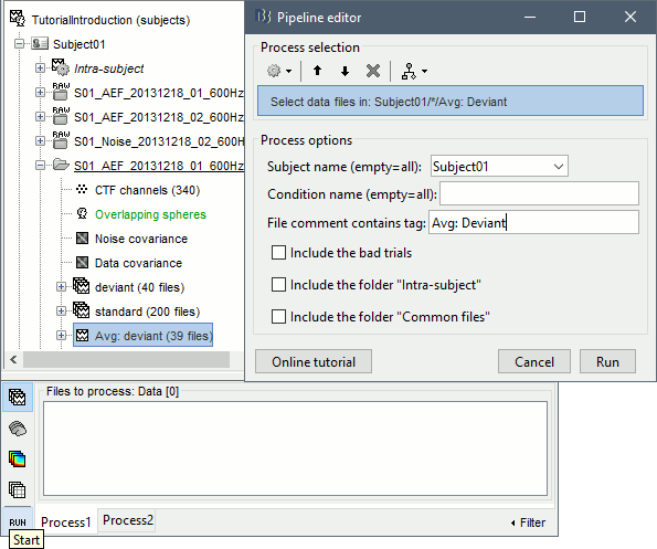
- This process selects all the recordings with a comment including the string "Avg: deviant", from all the folders in Subject01 (except for "Intra-subject" and "Common files"). We expect to get two files: the averages of the deviant condition for both runs.
Add process Pre-process > Band-pass filter: Lower cutoff=0Hz, Upper cutoff=30Hz, 60dB.
Add process File > Save snapshot: Recordings time series, Sensors=MEG.
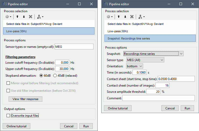
- This will apply a low-pass filter at 30Hz and save a screen capture of the signals in the report.
Do not run the pipeline, select the menu Generate .m script instead. It saves a new .m file and opens it in the Matlab editor. Close the pipeline editor window and look at the script.
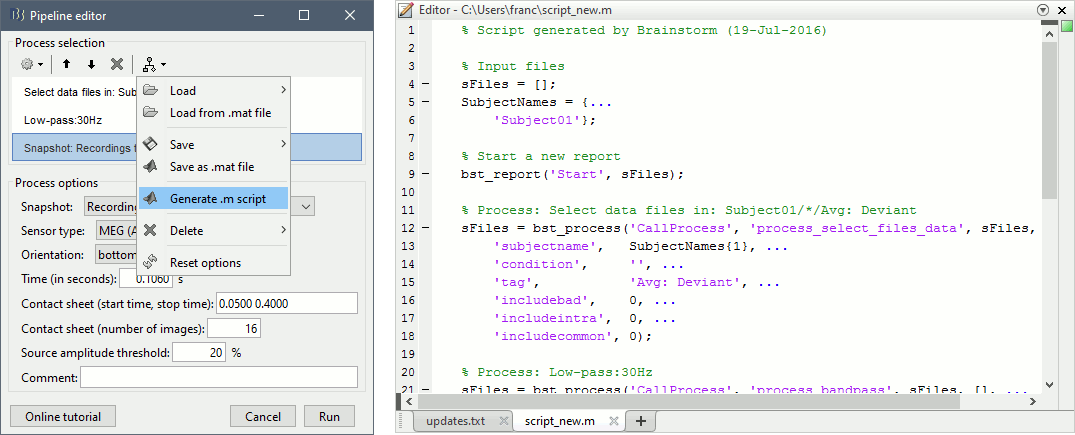
- The script you just generated can be the starting point to your own custom script. The following sections explain line by line how they work and how to edit them.
Line by line: Header
% Script generated by Brainstorm (19-Jul-2016)
All the lines starting with a "%" are comments, they are never executed.
% Input files
sFiles = [];
SubjectNames = {...
    'Subject01'};
These lines define the script inputs:
sFiles: The list of files in input. Currently empty because we did not select anything in the Process1 list. If we had selected files, it would contain a cell array of strings with relative file paths.
SubjectNames: List of subject names that are used in the script. Most of the times, the generated scripts contain only one entry, but it is written as a cell array to make it easier to extend to multiple subjects with a loop (described further in this tutorial).
% Start a new report
bst_report('Start', sFiles);
Starts a new report of activity: Clears all the previous logs and gets ready to record new messages. The report will collect all the messages that are generated during the execution of the script by the various processes. You can explicitly add screen captures and additional messages to the current report with the function bst_report. This report will remain open until the function bst_report('Start') is called again. To display the current report, use the menu File > Report viewer.
The syntax function_name('SubFunction', arguments) is used a lot in Brainstorm: it calls a subfunction available inside a .m file. This line above calls the function Start() in the file brainstorm3/toolbox/process/bst_report.m. This is made possible with the use of the short script "macro_method". Many of the Brainstorm .m files are actually libraries of functions, rather than simple "scripts" or "functions".
Line by line: Body
% Process: Select data files in: Subject01/*/Avg: deviant
sFiles = bst_process('CallProcess', 'process_select_files_data', sFiles, [], ...
    'subjectname',   SubjectNames{1}, ...
    'condition',     '', ...
    'tag',           'Avg: deviant', ...
    'includebad',    0, ...
    'includeintra',  0, ...
    'includecommon', 0);

% Process: Low-pass:30Hz
sFiles = bst_process('CallProcess', 'process_bandpass', sFiles, [], ...
    'sensortypes', 'MEG', ...
    'highpass',    0, ...
    'lowpass',     30, ...
    'attenuation', 'strict', ...  % 60dB
    'mirror',      0, ...
    'useold',      0, ...
    'overwrite',   0);

% Process: Snapshot: Recordings time series
sFiles = bst_process('CallProcess', 'process_snapshot', sFiles, [], ...
    'target',         5, ...  % Recordings time series
    'modality',       1, ...  % MEG (All)
    'orient',         4, ...  % bottom
    'time',           0.11, ...
    'contact_time',   [0, 0.1], ...
    'contact_nimage', 12, ...
    'threshold',      20, ...
    'Comment',        'Run');
You will find one block per process you selected in the pipeline editor. They all have the same syntax:
output_files = bst_process('CallProcess', process_name, input_files_A, input_files_B, options_list);
process_name: String indicating the function corresponding to the process to execute. To know from the pipeline editor what is the path to the process function: hover your mouse over the selected process, as illustrated in this tutorial.
input_files_A: List of input files in Process1, or FilesA in Process2. It can be a cell array of file names (full path, or relative path from the protocol folder), or an array of structures describing the files in the database (returned by a previous call to bst_process).
input_files_B: Empty for Process1, or FilesB in Process2. Cell array of strings, or array of struct.
options_list: Pairs of (option_name, option_values), one pair for each option of the process.
output_files: Array of structures describing the files in output of the process. If the process created new files, this variable points at them. If the process didn't create new files or was modifying exiting files, this variable points at the input files.
Line by line: Footer
% Save and display report
ReportFile = bst_report('Save', sFiles);
Closes the current report and saves it in the user report folder ($HOME/.brainstorm/reports). These reports are in .mat format and contain all the information necessary to re-run the execution exactly in the same way, but they are not easy to read.
The parameter "sFiles" is optional, it indicates what are the files that are considered as the final results of the script. You can remove it without breaking your script: ReportFile = bst_report('Save');
bst_report('Open', ReportFile);Opens the report viewer to display what happened during the execution. This is equivalent to using the menu File > Report viewer. You can comment this line (ie. add a "%" at the beginning of the line) if you don't want to show the report at the end of the execution.
% bst_report('Export', ReportFile, ExportDir);This function exports the report in readable format, as an HTML file that includes all the screen captures embedded in it. It is disabled by default. If you want to use this feature: remove the "%" at the beginning of the line, and define the variable ExportDir.
ExportDir must be a string that defines where to save the HTML report. It can be either the absolute path to a HTML file (eg. 'C:\Users\myuser\Documents\report_example.html') or just a folder (eg. 'C:\Users\myuser\Documents'). If you enter only a path to a folder, a default file name including the protocol name and a date tag is generated (report_ProtocolName_YYMMDD_HHMMSS.html).
% bst_report('Email', ReportFile, username, to, subject, isFullReport);Sends the report by email, as explained in this later section: Send report by email.
% gui_brainstorm('EmptyTempFolder');Delete all the files in the Brainstorm temporary folder.
Simplify the calls
The script you generated is like any Matlab script: you can edit it, rename the variables, add tests and loops, etc. The first important thing to understand is how to edit the options and change the inputs/outputs. The script generator uses only one variable for all the file lists (sFiles) and the output process is always the input of the following process. This is usually too restrictive to write a full analysis script: we commonly need to have multiple lists of files or to run two different operations on the same file.
Let's consider the first process call, which selects the averages for the Deviant condition in both runs.
sFiles = bst_process('CallProcess', 'process_select_files_data', sFiles, [], ...
    'subjectname',   SubjectNames{1}, ...
    'condition',     '', ...
    'tag',           'Avg: deviant', ...
    'includebad',    0, ...
    'includeintra',  0, ...
    'includecommon', 0);
There is no need to set the parameter sFiles, because there is no input, you can replace it with an empty matrix []. You can therefore remove the line "sFiles = [];". We can also rename the output variable "sAvgData", to be more specific.
sAvgData = bst_process('CallProcess', 'process_select_files_data', [], [], ...You can omit all the options that are not defined, not used, or kept to their default values:
sAvgData = bst_process('CallProcess', 'process_select_files_data', [], [], ...
    'subjectname',   SubjectNames{1}, ...
    'tag',           'Avg: deviant');
Edit the call to the low-pass filter: Change the input to sAvgData and the output to sAvgDataLow, this way you will be able to keep track of the two files if you need to use them independently later.
sAvgDataLow = bst_process('CallProcess', 'process_bandpass', sAvgData, [], ...
    'sensortypes', 'MEG', ...
    'highpass',    0, ...
    'lowpass',     30, ...
    'attenuation', 'strict');   % 60dB
Edit the call to the snapshot process: Change the input to sAvgDataLow, and remove the output parameter (we are not expecting any output file from it).
bst_process('CallProcess', 'process_snapshot', sAvgDataLow, [], ...
    'target',   5, ...  % Recordings time series
    'modality', 1);     % MEG (All)
Replace the last lines with the following code, in order to export the report instead of opening in the report viewer (edit the file path to point at your own user folder instead).
ReportFile = bst_report('Save');
bst_report('Export', ReportFile, 'C:\Users\myuser\Documents\report_test.html');
Evaluate in Matlab
Select the code for the first process in the Matlab editor, right-click > Evaluate selection (or press F9).

If you haven't executed your script yet, you will get the following error in the Matlab command window:
Undefined variable "SubjectNames" or class "SubjectNames".
The variable SubjectNames is not defined yet: Execute the first lines "SubjectNames = {'Subject01'}", then try again. You should now have a new variable in your Matlab workspace, which points at the two average files. Type "sAvgData(1)" in your command window to display the first element:
>> sAvgData(1)
ans =
          iStudy: 6
           iItem: 1
        FileName: '..._01_600Hz_notch/data_deviant_average_160513_1329.mat'
        FileType: 'data'
         Comment: 'Avg: deviant (39 files)'
       Condition: 'S01_AEF_20131218_01_600Hz_notch'
     SubjectFile: 'Subject01/brainstormsubject.mat'
     SubjectName: 'Subject01'
        DataFile: ''
     ChannelFile: 'Subject01/S01_AEF_20131218_01_600Hz_notch/channel_ctf_acc1.mat'
    ChannelTypes: {'ADC A'  'ADC V'  'DAC'  'ECG'  'EOG'  'MEG'  'MEG REF' ...}
The field "sAvgData(1).FileName" contains the relative path to the to the Deviant average in the first run. This structure sAvgData contains also a lot of information that can be helpful in your script:
iStudy / iItem: Reference of the file in the database (described later in this tutorial).
FileType: 'raw' (continuous files), 'data' (recordings), 'results' (sources), 'timefreq' (time-frequency, spectrum and connectivity), or 'matrix' (any time series extracted from other files).
Comment: Comment/Name field of the file (what is displayed in the database explorer).
Condition: Name of the condition/folder in which the file is located.
SubjectFile: Relative path to the subject file (brainstormsubject.mat).
SubjectName: Name of the subject (must be the same as the folder name).
DataFile: For types 'results' or 'timefreq', path of the parent file in the database explorer.
ChannelFile: Relative path to the channel file.
ChannelTypes: Cell array of channel types available for the input file.
Naming conventions
To help you navigate in the Brainstorm code, here are some, naming conventions (aka nomenclature):
Structures: Name starting with a "s" followed by a capital letter (eg. sFiles, sStudy, sSubject).
Indices: Either loop variables or array indices, name starting with a "i" (eg. iSubject, iStudy, iTime).
Counts: Number of elements in a group, name starting with a "n" (eg. nAvg, nTrials, nSubjects).
Graphic handles: Matlab graphic objects, name starting with a "h" (eg. hFig, hAxes, hLine, hText).
File names: Scripts and functions, only lower case, separation with "_" (eg. process_fft, bst_get).
Sub-functions: Inside a .m file, name starting with a capital, CamelCase (eg. CallProcess, Start).
Running the script
The simplified script looks like this:
% Input files
SubjectNames = {'Subject01'};
% Start a new report
bst_report('Start');

% Process: Select data files in: Subject01/*/Avg: deviant
sAvgData = bst_process('CallProcess', 'process_select_files_data', [], [], ...
    'subjectname',   SubjectNames{1}, ...
    'tag',           'Avg: deviant');
% Process: Low-pass:30Hz
sAvgDataLow = bst_process('CallProcess', 'process_bandpass', sAvgData, [], ...
    'sensortypes', 'MEG', ...
    'highpass',    0, ...
    'lowpass',     30, ...
    'attenuation', 'strict');  % 60dB
% Process: Snapshot: Recordings time series
bst_process('CallProcess', 'process_snapshot', sAvgDataLow, [], ...
    'target',   5, ...  % Recordings time series
    'modality', 1);     % MEG (All)

% Save and display report
ReportFile = bst_report('Save');
bst_report('Export', ReportFile, 'C:\Users\franc\Documents\report_test.html');
You have three ways to execute it:
- Select all the lines (Ctrl+A) and evaluate it in Matlab (F9).
- In the Editor toolbar of the Matlab environment, click on the button [Run].
- Save the file, go to this folder with Matlab (or add it to your path) and type the name of the script in the command window (without the ".m" at the end).
At the end of the execution, nothing happens, because we indicated we wanted to export the report instead of opening it. To check out the report of execution: use the menu File > Report viewer from the Brainstorm window, or open the file report_test.html that was saved somewhere on your computer.
In this page, you can review everything that happened in the script: when it was executed, how long it took, what are the processes that were executed, some additional messages (two files were selected with the first process) and the screen captures taken by process_snapshot.
Running the script again
If you execute the script again, it will not behave as expected anymore. The selection process we used assumes that there is only one file per folder with a name that includes "Avg: deviant". This is not the case anymore after the execution, because the low-pass filtered files also contain the same string. The execution of the first process of the script now returns 4 files.
>> sAvgData = bst_process('CallProcess', 'process_select_files_data', [], [], ...
    'subjectname',   SubjectNames{1}, ...
    'tag',           'Avg: deviant')

sAvgData =
1x4 struct array with fields:
    iStudy
    iItem
    ...
In order to exclude the low-pass filtered files from this selection, you can add another process that will refine the selection. Use the script generator again to create a template call for another process, then copy-paste it in your script.
- In Process1: Select any recordings file (we will not run anything, just generate a script).
Select process File > Select files: By tag: Search="low", Search the file name, Ignore the files.
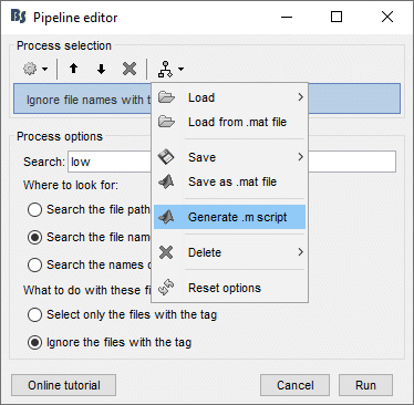
Select the menu Generate .m script (make sure you do not overwrite the script you are currently working on), then close the pipeline editor.
- Copy-paste and edit the call to process_select_tag to your main script.
Now the file selection part of your script should look like this, and should return only two files:
% Process: Select data files in: Subject01/*/Avg: Deviant
sAvgData = bst_process('CallProcess', 'process_select_files_data', [], [], ...
    'subjectname',   SubjectNames{1}, ...
    'tag',           'Avg: deviant');
% Process: Ignore file names with tag: low
sAvgData = bst_process('CallProcess', 'process_select_tag', sAvgData, [], ...
    'tag',    'low', ...
    'search', 2, ...  % Search the file names
    'select', 2);  % Ignore the files with the tag
With this last modification, your script is more robust. It can be executed multiple times without completely changing its behavior. When you are fetching files from the database using tags or file names, always pay attention to this aspect: the database grows and the further you go, the more specific your requests have to be.
A good practice can be to tag explicitly the output files your script generates if you need to fetch them later. You can use the process File > Add tag and File > Set name.
Starting Brainstorm
Brainstorm must be running in the background for these scripts to run properly. The interface doesn't have to be visible on the screen, but the database engine must be running for processing requests. At the beginning of your script, you can explicitly start or restart Brainstorm.
brainstorm: Start Brainstorm with the regular GUI.
brainstorm nogui: Start in silent mode. The Java GUI is created but hidden, the progress bar is not shown, all the processes run without user interactions, using default options instead of asking interactively. Visualization figures opened in the processing scripts are still created and made visible.
brainstorm server: Start in headless mode, for execution on a distant computation server that does not have any graphical capability or display attached to it. In this mode, none of the Java GUI elements are created, and the Matlab figures are not displayed. Whether you would be able to add screen captures to your execution reports depends mostly on the Matlab version available of your server (see section below Running scripts on a cluster).
brainstorm <script.m> <parameters>: Start Brainstorm in server mode, execute a script and quit Brainstorm. This allows executing any Matlab or Brainstorm script from the command line. This works also from the compiled version of Brainstorm, executed with the free MATLAB Runtime (see installation instructions, section "without Matlab"). Add the full path to the script and parameters to the command line:
Windows: brainstorm3.bat <script.m> <parameters>
Linux/MacOS: brainstorm3.command <MATLABROOT> <script.m> <parameters>
MATLABROOT: Matlab Runtime installation folder, eg. /usr/local/MATLAB_Runtime/v98/
brainstorm ... local: Instead of using a user defined brainstorm_db folder, it would use the default folder for the database: $HOME/.brainstorm/local_db
If you want to start Brainstorm only if it is not already running, you can use the following code:
if ~brainstorm('status')
    brainstorm nogui
end
To select a specific protocol at the beginning of your script:
ProtocolName = 'TutorialIntroduction';
% Get the protocol index
iProtocol = bst_get('Protocol', ProtocolName);
if isempty(iProtocol)
    error(['Unknown protocol: ' ProtocolName]);
end
% Select the current procotol
gui_brainstorm('SetCurrentProtocol', iProtocol);
To delete the protocol and start over:
% Delete existing protocol
gui_brainstorm('DeleteProtocol', ProtocolName);
% Create new protocol
gui_brainstorm('CreateProtocol', ProtocolName, 0, 0);
Additional command line options:
brainstorm stop      % Quit Brainstorm
brainstorm update    % Download and install latest Brainstorm update (see bst_update)
brainstorm reset     % Re-initialize Brainstorm database and preferences
brainstorm digitize  % Digitize electrodes positions and head shape using a Polhemus
brainstorm setpath   % Add Brainstorm subdirectories to current path
brainstorm info      % Open Brainstorm website
brainstorm forum     % Open Brainstorm forum
brainstorm license   % Display license
Database requests
The functions bst_get and bst_set allow you to query the database, access the configuration of the software and modify some display parameters. The complete reference documentation of these functions is included directly in their code (brainstorm3/toolbox/core/bst_get.m and bst_set.m).
Let's start with a few simple examples:
>> ProtocolInfo = bst_get('ProtocolInfo')  % Configuration of the current protocol
ProtocolInfo =
              Comment: 'TutorialIntroduction'
              STUDIES: 'C:\Work\Protocols\TutorialIntroduction\data'
             SUBJECTS: 'C:\Work\Protocols\TutorialIntroduction\anat'
               iStudy: 6
       UseDefaultAnat: 0
    UseDefaultChannel: 0

>> isGUI = bst_get('isGUI')   % Is the Brainstorm interface displayed (0=no, 1=yes)

>> bst_set('FlipYAxis', 1)                 % New figures will have the Y axis flipped
>> bst_set('TSDisplayMode', 'butterfly')   % New figures will use a "butterfly" view
To reference the files in the database, each protocol is subdivided in Subjects (the "anat" folder, containing the MRI, surfaces and atlases) and Studies (the "data" folder, including the recordings, channel files and all the analyses). Each Study corresponds to a sub-folder (eg. protocol/data/subject01/run01/), and is attached to only one subject.
Subjects and Studies are referenced in the protocol with a unique index, most of the time kept in variables named iSubject and iStudy. The files available in them are also referenced with indices, with variables such as iAnatomy, iSurface, iData, iHeadModel, iResults or iTimefreq. You can see the indices in the database explorer by hovering your mouse over the nodes files and folders:

Example: Getting the study structure from the variable sAvgData, defined in the script:
>> sAvgData(1)
ans =
          iStudy: 6
           iItem: 1
           ...

>> sStudy = bst_get('Study', sAvgData(1).iStudy)   % Get study struct with its index
sStudy =
                 Name: 'S01_AEF_20131218_01_600Hz_notch'
             FileName: 'Subject01/S01_AEF_20131218_01_600Hz_notch/brainstormstudy.mat'
          DateOfStudy: '13-May-2016'
    BrainStormSubject: 'Subject01/brainstormsubject.mat'   % Subject filename
            Condition: {'S01_AEF_20131218_01_600Hz_notch'} % Name of the folder
              Channel: [1x1 struct]       % Channel file
             iChannel: []                 % Not used anymore
                 Data: [1x242 struct]     % List of "data" files in the folder
            HeadModel: [1x1 struct]       % List of head models in the folder
           iHeadModel: 1                  % Default head model (file in green)
               Result: [1x244 struct]     % List of source files and links
                 Stat: [1x0 struct]       % List of statistical results
                Image: [0x0 struct]       % List of images
             NoiseCov: [1x2 struct]       % Noise(1) and data(2) covariance files
              Dipoles: [0x0 struct]       % List of dipole files in the folder
             Timefreq: [1x247 struct]     % List of time-frequency files
               Matrix: [0x0 struct]       % List of "matrix" files in the folder
Example: Getting the data structure.
% Get the structure representing the file from sStudy
>> sData = sStudy.Data(sAvgData(1).iItem)
sData =
    FileName: '..._01_600Hz_notch/data_deviant_average_160513_1329.mat'
     Comment: 'Avg: deviant (39 files)'    % File name
    DataType: 'recordings'                 % Type of data in the file
    BadTrial: 0                            % If 1, the trial is marked as bad
Example: Getting the subject structure.
% Get subject structure from filename (lists the files in the subject folder)
>> sSubject = bst_get('Subject', sStudy.BrainStormSubject)
sSubject =
                 Name: 'Subject01'    % Subject name, same as folder name
             Comments: ''             % Not used much
             FileName: 'Subject01/brainstormsubject.mat'
    DateOfAcquisition: ''             % Not used anymore
              Anatomy: [1x1 struct]   % List of MRI volumes
              Surface: [1x9 struct]   % List of surfaces
             iAnatomy: 1              % Index of default MRI
               iScalp: 9              % Index of default head surface
              iCortex: 4              % Index of default cortex surface
          iInnerSkull: []             % Index of default inner skull surface
          iOuterSkull: []             % Index of default outer skull surface
               iOther: []             % Not used anymore
       UseDefaultAnat: 0        % If 1: Use the default anatomy
    UseDefaultChannel: 0        % 0=one/folder, 1=one/subject, 2=one global
Example: Getting the study structure and data index from a file name.
>> DataFile = sAvgData(1).FileName
DataFile =
Subject01/..._01_600Hz_notch/data_deviant_average_160513_1329.mat

>> [sStudy, iStudy, iData] = bst_get('DataFile', DataFile)
sStudy =
                 Name: 'S01_AEF_20131218_01_600Hz_notch'
             FileName: '..._01_600Hz_notch/brainstormstudy.mat'
          DateOfStudy: '13-May-2016'
    BrainStormSubject: 'Subject01/brainstormsubject.mat'
            Condition: {'S01_AEF_20131218_01_600Hz_notch'}
              Channel: [1x1 struct]
             iChannel: []
                 Data: [1x242 struct]
            HeadModel: [1x1 struct]
           iHeadModel: 1
               Result: [1x244 struct]
                 Stat: [1x0 struct]
                Image: [0x0 struct]
             NoiseCov: [1x2 struct]
              Dipoles: [0x0 struct]
             Timefreq: [1x247 struct]
               Matrix: [0x0 struct]
iStudy =
     6
iData =
     1
Many other options are available for searching files in the database with bst_get. We cannot list them all in this page, but you can refer to the code of bst_get.m for more information.
To change parameters or database structures: bst_set.m.
File structures
The structures of the different types of files were described in the sections "On the hard drive" of the introduction tutorials. Here is a summary of all these sections:
Continuous recordings: File type "raw", Event markers.
Imported recordings: File type "data", Import epochs and Average response.
Power spectrum: File type "timefreq", Power spectrum and frequency filters.
Channel files: File type "channel", Channel file / MEG-MRI coregistration.
SSP/ICA projectors: Saved in the channel files, Artifact cleaning with SSP.
Head models: File type "headmodel", Head model.
Noise covariance: File types "noisecov" and "ndatacov", Noise and data covariance matrices.
Source files: File types "results" and "link", Source estimation.
Time-frequency: File type "timefreq", Time-frequency.
Statistics: File types "pdata", "presults", "ptimefreq" and "pmatrix", Statistics.
MRI volumes: File type "subjectimage", Display the anatomy.
Surfaces: File type "tess", Display the anatomy.
Scouts and atlases: Saved in the surface files, Scouts.
Custom processing
In many situations, you will find useful to read the files available in the database, and maybe modify them. The easiest approaches do not require any scripting, we will start by reviewing them quickly.
Process: Run Matlab command
If you want to modify the values saved in a file (eg. the field "F" from a "data" file), the easiest way is probably to use the process1 File > Run Matlab command. It is also available from Process2 in the category "Other".
It loads the files in input and run them through a piece of Matlab code that you can edit freely. It can extend a lot the flexibility of the Brainstorm pipeline manager, providing an easy access to any Matlab function or script.
The corresponding script looks like this:
sFiles = bst_process('CallProcess', 'process_matlab_eval', sFiles, [], ...
    'matlab',      'Data = Data.^2;', ...
    'sensortypes', 'MEG', ...
    'overwrite',   0);
Export/Import with the database explorer
Matlab
Right-click on the Deviant average in the database explorer > File > Export to Matlab > "DataMat".
Data exported as "DataMat"
>> DataMat
DataMat =
     ChannelFlag: [340x1 double]
    ColormapType: []
         Comment: 'Avg: deviant (39 files)'
        DataType: 'recordings'
          Device: 'CTF'
    DisplayUnits: []
               F: [340x361 double]
         History: {45x3 cell}
             Std: []
            Time: [1x361 double]
            nAvg: 39
          Events: [1x1 struct]
DataMat is the exact content of the corresponding .mat file, as loaded with Matlab's load() function. Edit some of the fields of this structure from the Matlab command window:
>> DataMat.Comment = 'Test square';
>> DataMat.F = DataMat.F .^ 2;
Now right-click on the folder containing the original file > File > Import from Matlab > DataMat:

If instead, you right-click on the original file and select the menu File > Import from Matlab, it overwrites the selected file instead of creating a new one with the selected structure.
Files
In addtion to export to Matlab, files in the database explorer can be exported as files. Right-click on the Deviant average in the database explorer > File > Export to File. Indicate the filename of the file format for the destination folder. The available file formats depend on the type of file to export.
Also, 'data' (raw and imported/trial recordings), 'results' (sources), 'timefreq' (time-frequency, spectrum and connectivity), or 'matrix' (any time series extracted from other files) files can be also exported to files using the process: File > Export to file .
Reference: File manipulation
Useful functions for manipulating file names and paths (read the code of the functions for help):
file_fullpath: Converts a relative file path to an absolute path.
file_short: Converts an absolute file path to a short path, relative to the current protocol folder.
file_gettype: Returns the type of a file.
Reading files from a script (all the functions take relative paths in input):
in_tess_bst(TessFile): Read a surface file.
in_mri_bst(MriFile): Read a MRI/volume file.
in_bst_data(DataFile): Read an imported epoch.
in_bst_timefreq(TimefreqFile): Read a power spectrum, time-frequency or connectivity file.
in_bst_channel(ChannelFile): Read a channel file.
in_bst_headmodel(HeadmodelFile, ApplyOrient): Read a head model file and apply orientations.
in_bst_results(ResultsFile, LoadFull): Load a source file and optionally reconstruct the full source time series on the fly (ImagingKernel * recordings).
in_bst_matrix(MatrixFile): Read a file with the type "matrix".
in_bst(FileName, TimeWindow): Read any Brainstorm data file with the possibility to load only a specific part of the file. "TimeWindow" is a range of time values in seconds: [tStart, tStop].
bst_process('LoadInputFile', FileName, Target, TimeWindow): The most high-level function for reading data files. "Target" is a string with the list of signal names or types to load.
bst_memory('GetConnectMatrix', TimefreqMat): Rebuild a full connectivity matrix.
in_fopen(DataFile, FileFormat, ImportOptions): Low-level function for opening continuous files.
in_fread(sFile, ChannelMat, iEpoch, SamplesBounds, iChannels, ImportOptions): Low-level function for reading blocks from continuous files. Requires a call to in_fopen first to get the sFile structure.
Saving files:
bst_save(FileName, FileMat, Version, isAppend): Save a file but does not register it in the database.
FileName: Absolute path to a .mat file, use in combination with file_fullpath for relative paths.
FileMat: Valid Brainstorm structure, corresponding to the file type.
Version: Defines which version of the Matlab .mat format is used to store the data:
- 'v6': Fastest option, bigger files, no compression, no files >2Gb
- 'v7': Slower option, compressed, no files >2Gb
- 'v7.3': Much slower than the others, compressed, but only way to save files > 2Gb.isAppend: If set to 1, updates only the fields defined in FileMat, keep the others untouched.
file_unique: Produces a unique file name by adding a number tag to it.
bst_process('GetNewFilename', OutputFolder, BaseFilename): Generate a new unique file name based on the beginning of the file name (eg. BaseFilename='data_average_test_').
Registering new files in the database:
db_add(iStudy/iSubject, FileMat): Add a new file in an anatomy folder or a functional data folder. This function saves the file and then reloads the folder. FileMat must be a structure, not a filename. You should not save the file manually before calling this function.
db_add_data(iStudy, FileName, FileMat): Register in the database a structure FileMat that has already been saved in file FileName. You should call bst_save manually before calling this function.
db_add_data(iStudy, FileName, FileMat, iItem): Overwrites the existing file #iItem.
Reload folders (if you saved or deleted files without registering correctly the modification in the database):
db_reload_studies(iStudies): Reload only the select data folders (aka "studies").
db_reload_conditions(iSubjects): Reload all the data folders for a subject.
db_reload_subjects(iSubjects): Reload the anatomy of the selected subjects.
db_reload_database('current'): Reload the entire protocol (anatomy and functional data).
Other useful database functions:
db_add_condition: Create a new folder in a subject.
db_add_subject: Create a new subject.
db_delete_studies: Delete a list of folders.
db_delete_subjects: Delete a list of subjects.
db_group_conditions: Merge two folders from the same subject.
db_rename_condition: Rename a folder.
db_rename_subject: Rename a subject.
db_set_channel: Set the channel file for a folder.
db_set_headmodel: Copy a head model to other folders
db_set_noisecov: Set the noise/data covariance for a folder, or copy to other folders/subjects.
db_set_template: Copy an anatomy template to a subject or use it as the default anatomy.
Export a file from the database to other file formats (read the comments in the functions for help):
- export_channel
- export_data
- export_events
- export_result
- export_timefreq
- export_matrix
- export_mri
- export_surfaces
- export_protocol: Export a subject or an entire protocol as a .zip file.
Convert Brainstorm structures to FieldTrip structures:
- out_fieldtrip_channel
- out_fieldtrip_data
- out_fieldtrip_timefreq
- out_fieldtrip_headmodel
- out_fieldtrip_results
- out_fieldtrip_matrix
Reference: Display functions
Create new visualization figures:
view_channels: Display sensors in a 3D figure.
view_helmet: Display the inner surface of the MEG helmet in a 3D figure.
view_timeseries: Display a data file as time series.
view_timeseries_matrix: Display a custom matrix as time series.
view_topography: Display a data file as a spatial topography.
view_erpimage: Display multiple data files as an image, signal by signal.
view_timefreq: Open a time-frequency file (various display modes available).
view_spectrum: Display a power spectrum (PSD or time-frequency files).
view_connect: Open a connectivity matrix (various display modes available).
view_matrix: Open a "matrix" file (various display modes available).
view_contactsheet: Create a contact sheet in time or across a volume from an existing figure.
view_noisecov: Display a noise or data covariance file.
view_dipoles: Open a dipoles file (various display modes available).
view_pac: Open PAC results (various display modes available).
view_mri: View a MRI file in the MRI viewer (with or without a functional overlay from a source file).
view_mri_3d: View a MRI file in a 3D figure (with or without a functional overlay from a source file).
view_surface: View a surface.
view_surface_data: View a surface file with a source file as its texture.
view_surface_matrix: View a custom surface (user defines vertices, faces, color, transparency).
view_image_reg: Display a 3D or 4D matrix as an image with time and/or frequency dimensions.
view_struct: Display a structure as with the popup menu "File > View file contents".
script_view_sources: Shortcut script to display source files.
bst_memory('UnloadAll', 'Forced'): Close all the existing figures.
Configure time-series figures:
panel_time('SetCurrentTime', t): Set current time.
panel_record('SetTimeLength', duration): Set the length of the current display page, in seconds.
panel_record('SetStartTime', t): Set the start of the current page, in seconds.
panel_record('SetDisplayMode', hFig, DisplayMode): 'column' or 'butterfly'.
panel_filter('SetFilters', isLowPass, LowPass, isHighPass, HighPass, isSinRem, SinRem, isMirror)
panel_montage('SetCurrentMontage', hFig, MontageName): Change the montage of channels.
bst_figures('SetSelectedRows', SelectedChannels): Set selected channels (cell array of strings).
figure_timeseries('SetTimeSelectionManual', hFig, TimeWindow): Select a time segment.
Configure 3D figures:
figure_3d('SetStandardView', hFig, 'left'): Change camera view (top,bottom,left,right,front,back).
figure_3d('ViewSensors', hFig, isMarkers, isLabels): Enable the view of sensor markers and labels.
panel_surface('SetShowSulci', hFig, iTess, 1): Show/hide the sulci (darker color for deeper areas).
panel_surface('SetSurfaceColor', hFig, iTess, [1 0 0]): Set the surface color.
panel_surface('SetSurfaceSmooth', hFig, iTess, Smooth, 0): Set the amount of smoothing (0-1).
panel_surface('SetSurfaceTransparency', hFig, iTess, Transp): Set the surface transparency (0-1).
panel_surface('SetDataThreshold', hFig, iTess, Thresh): Set the amplitude threshold.
panel_surface('SetSizeThreshold', hFig, iTess, MinSize): Set size threshold (min size slider).
panel_surface('SelectHemispheres', target): Equivalent to clicking on the buttons in the Resect panel of the Surface tab. Possible target values: 'left', 'right', 'struct', 'none'
figure_mri('SetLocation', CsName, hFig, [], xyz): CsName=voxel/mri/scs/mni, xyz=[x,y,z]
Configure time-frequency figures:
panel_freq('SetCurrentFreq', iFreq, 1): Set the current frequency index (from the Freqs vector)
panel_freq('SetCurrentFreq', Freq, 0): Set the current frequency (in Hz).
sOptions = panel_display('GetDisplayOptions'): Get display options selected in the Display tab.
panel_display('SetDisplayOptions', sOptions): Change the options selected in the Display tab.
sOptions.HideEdgeEffects: Controls the checkbox "Hide edge effects" (0 or 1).
sOptions.HighResolution: Controls the checkbox "Smooth display" (0 or 1).
sOptions.RowName: Controls the signal that is currently displayed (for 'SingleSensor' display mode).
sOptions.Function: Controls the display function (magnitude, power, log, phase).
Configure colormaps:
bst_colormaps('SetColormapName', ColormapType, ColormapName): 'jet', 'parula', 'cmap_rbw', ...
bst_colormaps('SetMaxMode', ColormapType, MaxMode): Colorbar range ('global', 'local', 'custom').
bst_colormaps('SetMaxCustom', ColormapType, [], Min, Max): Set a custom colorbar range.
bst_colormaps('SetColormapAbsolute', ColormapType, isAbsolute): Show positive or relative values
bst_colormaps('SetDisplayColorbar', ColormapType, isDisplay): Show colorbar in the figures.
bst_colormaps('RestoreDefaults', ColormapType): Restore the default configuration for a colormap.
ColormapType: anatomy, meg, eeg, sources, stat1, stat2, time, timefreq, connect1, connectn, image
Configure statistical thresholding:
StatThreshOptions = bst_get('StatThreshOptions'): Get display options selected in the Stat tab.
bst_set('StatThreshOptions', StatThreshOptions): Change the options selected in the Stat tab.
StatThreshOptions.pThreshold: Current significance level α (ie. p-value threshold)
StatThreshOptions.Correction: Correction for multiple comparisons ('none', 'fdr', 'bonferroni')
StatThreshOptions.Control: List of dimensions to correct for multiple comparisons (default = [1 2 3])
Export the contents of a figure to a file:
out_figure_image: Screen capture of any Brainstorm figure.
out_figure_movie: Save a movie from one or multiple Brainstorm figures.
out_figure_timefreq: Extract some of the data displayed in a time-frequency figure.
out_figure_timeseries: Extract some of the data displayed in a time series figure.
Example: Creating a new file
This section illustrates how to add new files to the database. We will create a sinusoidal signal and save it in a "matrix" file, in a new folder of the subject "Test".
% Time: 1 second with a sampling frequency of 1000Hz
t = 0:0.001:1;
% Generate two sinsuoidal signals (20Hz,30Hz)
F = [sin(20*2*pi*t); 0.5*sin(30*2*pi*t)];

% Initialize an empty "matrix" structure
sMat = db_template('matrixmat');
% Fill the required fields of the structure
sMat.Value       = F;
sMat.Comment     = 'Test sinusoids';
sMat.Description = {'Signal #1: 20Hz'; 'Signal #2: 30Hz'};
sMat.Time        = t;

% Create a new folder "Script" in subject "Test"
iStudy = db_add_condition('Test', 'Script');
% Get the corresponding study structure
sStudy = bst_get('Study', iStudy);
There are many options to add a new file to the database, with various levels of requirements. You can call the db_add function (reloads the destination folder, therefore slow if you save many files), save the file in the corresponding folder and reload the protocol (slow as well), or register the file in the database manually (more complicated but faster).
Option #1: db_add
OutputFile = db_add(iStudy, sMat);
Option #2: bst_save / db_reload_studies
% Get the full path to the new folder
% (same folder as the brainstormstudy.mat file for this study)
OutputFolder = bst_fileparts(file_fullpath(sStudy.FileName));
% Get a new unique filename (including a timestamp)
MatrixFile = bst_process('GetNewFilename', OutputFolder, 'matrix_test');
% Save file
bst_save(MatrixFile, sMat, 'v6');
% Reload the folder in which the new file was saved
db_reload_studies(iStudy);
Option #3: bst_save / db_add_data
% Another way to generate a unique filename (without a timestamp)
MatrixFile = file_unique(bst_fullfile(OutputFolder, 'matrix_test.mat'));
% Save file
bst_save(MatrixFile, sMat, 'v6');
% Reference saved file in the database
db_add_data(iStudy, MatrixFile, sMat);
% Update the database explorer display
panel_protocols('UpdateNode', 'Study', iStudy);
Example: Editing events
A step that commonly requires manual changes is the definition of the event markers. For example, we have to combine external triggers or behavioral information with the existing events. This example illustrates how to load the events, modify them and save them back.
For the continuous recordings, the events are saved in the .mat file corresponding to the "Link to raw file". These structures contain only meta-data and information created with Brainstorm, the EEG/MEG recordings are available in a separate binary file. First, we need to load this link.
% Right-click on a "Link to raw file" in the database explorer
%  > File > Copy file path to clipboard
RawFile = '/.../@rawS01.../data_0raw_S01_..._01_600Hz_notch.mat'

% Load the "sFile" structure, contained in the .F structure
% of the link file (data_0raw...mat)
sRaw = in_bst_data(RawFile, 'F');

>> sRaw.F.events
ans =
1x7 struct array with fields:
    label
    color
    epochs
    times
    reactTimes
    select
    channels
    notes
For example, let's say we want to add 30ms to all the events in the category "button" in order to compensate for some hardware delay, and create a new event category with the modified timing. We need first to identify what is the index of the category "button", in this array of 7 event structures.
% Find the index of the event category "button"
iEvtButton = find(strcmpi({sRaw.F.events.label}, 'button'));

>> iEvtButton
iEvtButton =
     3
In the code above, note this special Matlab syntax that allows the concatenation of the values of one field across multiple structures, in an array of structures:
>> {sRaw.F.events.label}
ans =
    'standard'    'deviant'    'button'    'cardiac'
    'blink'    'bad_1-7Hz'    'bad_40-240Hz'
If you want to search instead all the events containing a specific tag, for example "bad", you can use the cellfun function (applies the same function sequentially to all the elements in a cell array and concatenates the results) in combination with the strfind function (search for a substring). The final call to the find function returns at which indices the list of tags found in the event label is not empty.
>> iEvtBad = find( ~cellfun( @(c)isempty(strfind(c,'bad')), ...
                             {sRaw.F.events.label}))
iEvtBad =
     6     7
The code below copies the existing event category "button", renames it and add a 30ms offset. If you add or remove events, you must adjust the size of the other fields: epochs (always 1 for most file formats), channels and notes (cell array of empty matrices in most cases).
% Copy the event category "button" to a new category
iEvtNew = length(sRaw.F.events) + 1;
sRaw.F.events(iEvtNew) = sRaw.F.events(iEvtButton);
% Rename the new event to "button_offset"
sRaw.F.events(iEvtNew).label = 'button_offset';

% How many samples in 30ms (0.030s * 600Hz = 18 samples)
offsetSample = round(0.030 .* sRaw.F.prop.sfreq);
% Apply offset to the events in the "button_offset" category
sRaw.F.events(iEvtNew).times = sRaw.F.events(iEvtNew).times + 0.03
% Round new time values to the nearest sample
sRaw.F.events(iEvtNew).times = ...
    round(sRaw.F.events(iEvtNew).times .* sRaw.F.prop.sfreq) ./ sRaw.F.prop.sfreq;
% Re-generate an epochs field with only ones, and empty notes and channels fields
% (optional here, as we didn't change the number of evt)
nTimes = size(sRaw.F.events(iEvtNew).times, 2);
sRaw.F.events(iEvtNew).epochs = ones(1, nTimes);
sRaw.F.events(iEvtNew).channels = cell(1, nTimes);
sRaw.F.events(iEvtNew).notes = cell(1, nTimes);
% Change the event color to yellow (red=1, green=1, blue=0)
sRaw.F.events(iEvtNew).color = [1 1 0];

>> sRaw.F.events(iEvtNew)
ans =
         label: 'button_offset'
         color: [1 1 0]
        epochs: [1x40 double]
         times: [1x40 double]
    reactTimes: []
        select: 1
      channels: {1x40 cell}
         notes: {1x40 cell}
The last step is to save the modifications back to the "Link to raw file". Here the call to file_fullpath is optional because the variable RawFile already contains the absolute path to the file.
% Update the sRaw structure to the RawFile file (the last parameter appends to the existing struct)
bst_save(file_fullpath(RawFile), sRaw, 'v6', 1);
Open the recordings to make sure your transformation worked the way you expected.
Find examples in the code
The easier way to understand how to use a function is to search the code with the "Find files" interface in Matlab. Go to the brainstorm3 folder, click on "Find files" (or Ctrl+Shift+F), enter the name of a function in "Find files containing text", Include subfolders, Match case. It will return all the lines that include the string you entered across all the files in the Brainstorm distribution. Just double-click on a line to jump to the code in the Matlab editor.
You can use the same interface to find what function is called when you click on a button or menu in the interface. Search for the label or the tooltip of the interface element in the same way. The example below shows how to track what happens when you click on the headmodel popup menu "Check spheres".

If you have trouble understanding how to set some input parameters, you can use the Matlab's debugger to explore a real use case. Place a breakpoint at the begging of your function of interest (watch this tutorial if you don't know how to do this), for example in view_timeseries.m. Then click on the corresponding menus in the Brainstorm interface (eg. double-click on a data file). When the execution reaches the line you selected, it stops and gives you back the commands. You can explore the values in all the variables, modify them, and execute the code step by step (many options available in the Editor tab of Matlab).
Find interface callback functions
If you are looking for the function called by a menu or a button in the interface:
- In Matlab, go to the "brainstorm3" folder
- Click on the button "Find file" in the ribbon "Editor" of Matlab interface (Ctrl+Shift+F)
- Select the option "Include subfolders"
- Search for the text of the menu or button you are looking for (eg. 'Set as default'); you can do a case-sensitive or a case-insensitive search (option "Match case")
It gives you the list of all the places where this text appears in the Brainstorm code. In the previous example, in tree_callbacks.m, you’d find a call to function SetDefaultSurf.
- Double-click on the corresponding line to jump to the code
Right-click on "SetDefaultSurf" > Open "SetDefaultSurf"
The editor should jump to the code of function SetDefaultSurf(), and there you’d find your call to "db_surface_default"
Right-click on it > Open "db_surface_default" to open the function and read the header that should explain its usage (this example is not very detailed, sorry)
Sometimes it helps to look at other examples of calls to this function: Use the window "Find files" again to search for text "db_surface_default"
Additional quality control
You can add in the reports all the information that may help you control the quality of the analysis, or figures you want to include in publications or clinical reports. The process "File > Save snapshot" lets you save some predefined views, but you can also custom screen captures. The example below shows how to add a "raster plot" for all the deviant trials from Run#01 in the report.
% Get all the deviant trials in Run#01  (the list includes the deviant average)
sDeviant = bst_process('CallProcess', 'process_select_files_data', [], [], ...
    'subjectname',   'Subject01', ...
    'condition',     'S01_AEF_20131218_01_600Hz_notch', ...
    'tag',           'deviant');

% Open raster plot
hFig = view_erpimage({sDeviant.FileName}, 'erpimage', 'MEG');
% Select the channel MRT34
sOptions = panel_display('GetDisplayOptions');
sOptions.RowName = 'MRT34';
panel_display('SetDisplayOptions', sOptions);

% Screen capture of this figure
% bst_report('Snapshot', hFig, FileName, Comment, WindowPosition);
bst_report('Snapshot', hFig, [], 'ERP image: MRT34', [300 100 600 400]);
% Close figure
close(hFig);
You can also add messages in the reports (information, warning or errors).
% Function call: bst_report(MsgType, sProcess, sInputs, Message)
bst_report('Info',    [], sDeviant, 'This is an information message.');
bst_report('Warning', [], sDeviant, 'This is a warning.');
bst_report('Error',   [], sDeviant, 'This is an error.');

% Open the report viewer to show the current report (not saved yet)
bst_report('Open', 'Current');
Report generated with the code above:
Loop over subjects
Creating loops is not supported yet by the script generator, but relatively easy to do from a script without knowing too much about Matlab programming. The example below shows how to create a loop over subjects to import their anatomy. The dataset used here is from the tutorial MEG visual: single subject.
With the Process1 box empty, select the process "Import > Import anatomy > Import anatomy folder" and generate a script. Simplify if using the guidelines presented in the previous sections:
% Input files
SubjectNames = {'sub001'};
RawFiles = {...
    '/.../Tutorials/sample_group/freesurfer/sub001'};

% Process: Import anatomy folder
bst_process('CallProcess', 'process_import_anatomy', [], [], ...
    'subjectname', SubjectNames{1}, ...
    'mrifile',     {RawFiles{1}, 'FreeSurfer'}, ...
    'nvertices',   15000);
Add the other subject names and corresponding FreeSurfer folders in the script header:
SubjectNames = {'sub001', 'sub002', 'sub003', 'sub004'};
RawFiles = {...
    '/.../Tutorials/sample_group/freesurfer/sub001', ...
    '/.../Tutorials/sample_group/freesurfer/sub002', ...
    '/.../Tutorials/sample_group/freesurfer/sub003', ...
    '/.../Tutorials/sample_group/freesurfer/sub004'};
Add a for loop around all the steps to repeat on each subject ("for" before, and "end" after the code), and replace the indices "1" with the loop variable:
% Loop on subjects
for iSubject = 1:length(SubjectNames)
    % Process: Import anatomy folder
    bst_process('CallProcess', 'process_import_anatomy', [], [], ...
        'subjectname', SubjectNames{iSubject}, ...
        'mrifile',     {RawFiles{iSubject}, 'FreeSurfer'}, ...
        'nvertices',   15000);
end
Loop over acquisition runs
If you have multiple subjects for which the anatomy is already imported, and multiple runs to process for each subject, you can add two nested for loops to link all the runs to the database in the same script. The dataset used here is from the tutorial MEG visual: single subject.
With the Process1 box empty, select the process "Import > Import recordings > Create link to raw file" and generate a script. Simplify if using the guidelines presented in the previous sections:
% Input files
SubjectNames = {'sub001'};
RawFiles = {...
    '/.../sample_group/ds117/sub001/MEG/run_01_sss.fif'};

% Process: Create link to raw file
sFileRaw = bst_process('CallProcess', 'process_import_data_raw', [], [], ...
    'subjectname',    SubjectNames{1}, ...
    'datafile',       {RawFiles{1}, 'FIF'}, ...
    'channelreplace', 0, ...
    'channelalign',   0, ...
    'evtmode',        'value');
Add the other subject names and all the runs for all the subjects (array of cell arrays) in the script header:
SubjectNames = {'sub001', 'sub002'};
RawFiles = {...
    {'/.../sample_group/ds117/sub001/MEG/run_01_sss.fif', ...
     '/.../sample_group/ds117/sub001/MEG/run_02_sss.fif', ...
     '/.../sample_group/ds117/sub001/MEG/run_03_sss.fif'}, ...
    {'/.../sample_group/ds117/sub002/MEG/run_01_sss.fif', ...
     '/.../sample_group/ds117/sub002/MEG/run_02_sss.fif', ...
     '/.../sample_group/ds117/sub002/MEG/run_03_sss.fif'}};
Add two for loops around the code to repeat on all the runs:
% Loop on subjects
for iSubject = 1:length(SubjectNames)
  % Loop on runs for each subject
  for iRun = 1:length(RawFiles{iSubject})
    % Process: Create link to raw file
    sFileRaw = bst_process('CallProcess', 'process_import_data_raw', [], [], ...
        'subjectname',    SubjectNames{iSubject}, ...
        'datafile',       {RawFiles{iSubjects}{iRun}, 'FIF'}, ...
        'channelreplace', 0, ...
        'channelalign',   0, ...
        'evtmode',        'value');
  end
end
How to process an entire study
This section proposes a standard workflow for processing a full group study with Brainstorm. It contains the same steps of analysis as the introduction tutorials, but separating what can be done automatically from what should be done manually. This workflow can be adapted to most ERP studies (stimulus-based).
Prototype: Start by processing one or two subjects completely interactively (exactly like in the introduction tutorials). Use the few pilot subjects that you have for your study to prototype the analysis pipeline and check manually all the intermediate stages. Take notes of what you're doing along the way, so that you can later write a script that reproduces the same operations.
Anatomical fiducials: Set NAS/LPA/RPA and compute the MNI normalization for each subject.
Segmentation: Run FreeSurfer/BrainSuite to get surfaces and atlases for all the subjects.
File > Batch MRI fiducials: This menu prompts for the selection of the fiducials for all the subjects and saves a file fiducials.m in each segmentation folder. You will not have to redo this even if you have to start over your analysis from the beginning.
Script: Write a loop that calls the process "Import anatomy folder" for all the subjects.
Alternatives: Create and import the subjects one by one and set the fiducials at the import time. Or use the default anatomy for all the subjects (or use warped templates).
Script #1: Pre-processing: Loop on the subjects and the acquisition runs.
Create link to raw files: Link the subject and noise recordings to the database.
Event markers: Read and group triggers from digital and analog channel, fix stimulation delays
Evaluation: Power spectrum density of the recordings to evaluate their quality.
Pre-processing: Notch filter, sinusoid removal, band-pass filter.
Evaluation: Power spectrum density of the recordings to make sure the filters worked well.
Cleanup: Delete the links to the original files (the filtered ones are copied in the database).
Detect artifacts: Detect heartbeats, Detect eye blinks, Remove simultaneous.
Compute SSP: Heartbeats, Blinks (this selects the first component of each decomposition)
Compute ICA: If you have some artifacts you'd like to remove with ICA (no default selection).
Screenshots: Check the MRI/sensors registration, PSD before and after corrections, SSP.
Export the report: One report per subject, or one report for all the subjects, saved in HTML.
Manual inspection #1:
Check the reports: Information messages (number of events, errors and warnings) and screen captures (registration problems, obvious noisy channels, incorrect SSP topographies).
Mark bad channels: Open the recordings, select the channels and mark them as bad. Or use the process "Set bad channels" to mark the same bad channels in multiple files.
Fix the SSP/ICA: For the suspicious runs: Open the file, adjust the list of blink and cardiac events, remove and recompute the SSP decompositions, manually select the components.
Detect other artifacts: Run the process on all the runs of all the subjects at once (select all the files in Process1 and run the process, or generate the equivalent script).
Mark bad segments: Review the artifacts detected in 1-7Hz and 40-240Hz, keep only the ones you really want to remove, then mark the event categories as bad. Review quickly the rest of the file and check that there are no other important artifacts.
Additional SSP: If you find one type of artifact that repeats (typically saccades and SQUID jumps), you can create additional SSP projectors, either with the process "SSP: Generic" or directly from a topography figure (right-click on the figure > Snapshot> Use as SSP projector).
Script #2: Subject-level analysis: Epoching, averaging, sources, time-frequency.
Importing: Process "Import MEG/EEG: Events" and "Pre-process > Remove DC offset".
Averaging: Average trials by run, average runs by subject (registration problem in MEG).
Noise covariance: Compute from empty room or resting recordings, copy to other folders.
Head model: Compute for each run, or compute once and copy if the runs are co-registered.
Sources: Compute for each run, average across runs and subjects in source space for MEG.
Time-frequency: Computation with Hilbert transform or Morlet wavelets, then normalize.
Screenshots: Check the quality of all the averages (time series, topographies, sources).
Export the report: One report per subject, or one report for all the subjects, saved in HTML.
Manual inspection #2:
Check the reports: Check the number of epochs imported and averaged in each condition, check the screen capture of the averages (all the primary responses should be clearly visible).
Regions of interest: If not using predefined regions from an atlas, define the scouts on the anatomy of each subject (or on the template and then project them to the subjects).
Script #3: Group analysis, ROI-based analysis, etc.
Averaging: Group averages for the sensor data, the sources and the time-frequency maps.
Statistics: Contrast between conditions or groups of subjects.
Regions of interest: Any operation that involve scouts.
Final scripts
The following script from the Brainstorm distribution reproduces the introduction tutorials ("Get started"): brainstorm3/toolbox/script/tutorial_introduction.m - Report: report_TutorialIntroduction.html
For an example of a script illustrating how to create loops, look at the tutorial MEG visual: single subject. brainstorm3/toolbox/script/tutorial_visual_single.m - Report: report_TutorialVisual_sub001.html
Temporary files
Some processes need to create temporary files on the hard drive. For example, when epoching MEG/EEG recordings, Brainstorm would first create a temporary folder import_yymmdd_hhmmss, store all the epochs in it, then move them to the database when the epoching process is completed. The name of the temporary folder indicates its creation time (year/month/day_hour_minutes_seconds).
The default folder where Brainstorm stores its temporary files is located in the user folder ($HOME/.brainstorm/tmp/). This can be changed as explained in the introduction tutorial Create protocol.
At the end of each process, all the temporary files should be deleted automatically. However, in some cases, the process crashes or is killed before it can delete its temporary files. When starting the Brainstorm interface, users gets offered to delete the remaining temporary files. However, when running Brainstorm only from scripts, these files may never be deleted or made explicitly visible. To avoid these leftover temporary files to pile up indefinitely, it can be useful to add an explicit call to the function below, which deletes all of them.
gui_brainstorm('EmptyTempFolder');Warning: Do not call this function in scripts that are supposed to be executed in parallel from the same user, as it might delete the temporary files from another session of Brainstorm.
Parallel processing
At the moment, Brainstorm is not capable of safely handling multiple sessions executed on the same computer, from the same user or on the same database folder. We are working on a new version of the databasing system that will support concurrent accesses. Until this is released, you should not have multiple people working at the same time with the same database, or multiple Matlab/Brainstorm instances running in parallel.
In some specific cases, however, it is possible to start multiple long processes simultaneously without much risk. For example, starting the BrainSuite MRI segmentation for multiple subjects within the same protocol can make sense. Some recommendations to run this safely:
- The current protocol should never be changed
- The temporary files from the other processes should not be deleted
- Each instance of Matlab/Brainstorm must process a different subject
- Reload the database after all the executions are completed
Note that parallel processing does not always improve global performances. Many Matlab functions are already optimized to distribute their computation load over multiple CPUs. Running these in parallel from multiple instances of Matlab could be slower and less efficient in terms of memory usage, than running them sequentially from the same instance. Before deciding on running tasks in parallel, unless they are clearly not optimized to work on multiple cores (e.g. FreeSurfer segmentation), you should always run some tests to make sure it improves the global computation time.
Running scripts on a cluster
With Matlab
Matlab, including the toolboxes you need, needs to be installed on the server and a Brainstorm version needs to be located on the server. Start Brainstorm with the command "brainstorm server".
For the database: the folder "brainstorm_db" needs to be registered at the beginning of the script. You can either upload a protocol folder from your local computer, or create an empty brainstorm_db folder and a new protocol on the distance server. At the end of this initialization phase, you need to have something like the structure below:
/home/user/brainstorm3
/home/user/brainstorm_db/ProtocolName/anat
/home/user/brainstorm_db/ProtocolName/data
Your processing script could start with some of the elements below, depending on what you need:
% Start Brainstorm
cd /home/user/brainstorm3;
if ~brainstorm('status')
    brainstorm server
end

% Path to a Brainstorm database (= a folder that contains one or more Brainstorm protocols)
BrainstormDbDir = '/home/user/brainstorm_db';

% Load a new uploaded database (sets BrainstormDbDir and load all the protocols it contains)
db_import(BrainstormDbDir);

% Alternative: Set the Brainstorm DB folder
% (defines where the new protocols are going to be created, but does not load anything)
bst_set('BrainstormDbDir', BrainstormDbDir);

% Get the protocol index of an existing protocol (already loaded previously in Brainstorm)
iProtocol = bst_get('Protocol', ProtocolName);

% Create a new protocol if needed
if isempty(iProtocol)
    UseDefaultAnat = 0;
    UseDefaultChannel = 0;
    gui_brainstorm('CreateProtocol', ProtocolName, UseDefaultAnat, UseDefaultChannel);
end

% Delete an existing protocol
gui_brainstorm('DeleteProtocol', ProtocolName);
Execution: You should check that there is a Matlab license available on the server, and that RAM and disk quotas are large enough for the data you will create while processing. The Matlab version might differ from the version installed on your local computer or toolboxes might be missing, causing some errors.
A Brainstorm script can be executed either directly (it needs to start Brainstorm itself, like in the example script above), or started using the syntax brainstorm <script.m> <parameters> (starts Brainstorm in server mode, executes the script and quit Brainstorm). See sections Starting Brainstorm and Parameters.
External Matlab call
To call a Brainstorm script directly from the command line of a terminal and avoid the graphical environment of Matlab to get started, on Linux or MacOS, you can use the syntax:
matlab -nosplash -nodesktop -r "run('/path/to/script.m');"
Without Matlab
Brainstorm scripts can also be executed from the compiled version of Brainstorm, therefore not requiring a Matlab license, only the installation of the free MATLAB Runtime (see installation instructions, section "without Matlab"). Add the full path to the script and the parameters to the command line:
Windows: brainstorm3.bat <script.m> <parameters>
Linux/MacOS: brainstorm3.command <MATLABROOT> <script.m> <parameters>
MATLABROOT: Matlab Runtime installation folder, eg. /usr/local/MATLAB_Runtime/v98/To avoid being asked for "brainstorm_db", add the argument: local
Example: brainstorm3.command /usr/local/MATLAB/MATLAB_Runtime/v98 main.m local
In this configuration, Brainstorm is started using the command brainstorm server and then the script is executed. Therefore, your script should not start brainstorm again: remove the line "brainstorm server" from the example script in the section above.
In this configuration, the Matlab Runtime is not allowed to compile and execute .m scripts as a regular Matlab installation would. To work around this limitation, Brainstorm reads the script.m file and executes its contents with the Matlab eval function. Therefore this approach does not support the definition of functions or classes within the script.m. The compiled version of Brainstorm can only run code that can be executed from the Matlab Command Window. If you need more flexibility, you need to recompile a modified version of Brainstorm including your custom code (see below).
Parameters
The syntax of the script changes depending on the input parameters it accepts from the command line.
No extra parameters
The .m file must have the structure of a simple script, with no additional function definition.
Example script.m:
disp(['SCRIPT> Script start.']);
sStudy = bst_get('Study');
disp(['SCRIPT> Current study path: ' sStudy.FileName 10]);
Execution from the command line:
>> brainstorm 'C:\Users\franc\Downloads\GetStudyPath.m'

BST> Starting Brainstorm:
BST> =================================
BST> Version: 15-Jun-2022
BST> Deleting old process reports...
BST> Loading configuration file...
BST> Reading process folder...
BST> Loading current protocol...
BST> =================================

SCRIPT> Script start.
SCRIPT> Current study path: Subject01/S01_AEF_20131218_01_600Hz_notch/brainstormstudy.mat

BST> Emptying temporary directory...
BST> Brainstorm stopped.
Extra command line parameters
The .m file must declare a function on its first line. The number and names of parameters are parsed by Brainstorm from this first line, matched with the parameters passed from the command line, then the first line is removed and the rest of the code is executed with eval. Avoid including the "end" statement for the function, as it would result in more work to identify and remove it from the code. No other functions, sub-functions or classes can be declared in the same .m file.
Note that parameters are received as char arrays in the code: if you are expecting to pass numerical values, then the values must be parsed from the string (eg. with str2num).
Example script.m:
function GetStudyPath(iStudy)

disp([10 'SCRIPT> Script start.']);
sStudy = bst_get('Study', str2num(iStudy));
disp(['SCRIPT> Study path: ' sStudy.FileName 10]);
Execution from the command line:
>> brainstorm 'C:\Users\franc\Downloads\GetStudyPath.m' 1

BST> Starting Brainstorm:
BST> =================================
BST> Version: 15-Jun-2022
BST> Deleting old process reports...
BST> Loading configuration file...
BST> Reading process folder...
BST> Loading current protocol...
BST> =================================

WARNING: This file is a function, trying to convert to a script...

SCRIPT> Script start.
SCRIPT> Study path: Test/@default_study/brainstormstudy.mat

BST> Emptying temporary directory...
BST> Brainstorm stopped.
Send report by email
When running some long computation on a distant server, it can be convenient to receive an email when the processing is over. Two solutions for sending yourself an email from Brainstorm: from the pipeline editor, or directly from a script.
Use the process File > Send report by email to send the current execution report:
Brainstorm username: The user name you use to download Brainstorm from the website, or to post messages on the user forum. The email associated with this account is the primary recipient of the email.
Send copy to: Optional, sends a copy to an additional email address. Use this to notify collaborator, or receive the notification on an email address that is not registered on the Brainstorm website.
Subject: Subject of the email.
Send full report: If selected, sends the full HTML execution report as displayed by the Report viewer. Be careful when working with sensitive patient data, as it would send with no encryption the full file names of all the files. If not selected, only the name of the processes and execution times are sent, in plain text.
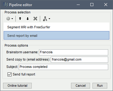
Alternatively, use one of the following options (isFullReport can be set to 0 or 1):
% At the end of your script
ReportFile = bst_report('Save', sFiles);
bst_report('Email', ReportFile, username, to, subject, isFullReport);

% Anywhere in your script
bst_report('Email', 'current', username, to, subject, isFullReport);
How to compile Brainstorm
Brainstorm can be compiled as a JAR application using the function bst_compile.m. You would need this in order to execute without Matlab a modified version of Brainstorm.
Software requirements:
MATLAB >= 2020a
- MATLAB Compiler toolbox
- MATLAB Compiler SDK toolbox
- OpenJDK 8:
- Install Ubuntu package: sudo apt install openjdk-8-jdk
Set the environment variable JAVA_HOME to the installation folder of the JDK.
Windows 10: Right-click on "This PC" > Advanced system settings > Environment variables
Linux & MacOS: The syntax depends on your shell, look it up on Google.
- From Matlab: setenv('JAVA_HOME', '/path/to/jdk-8.0.../')
- Check the environment variable from Matlab: getenv('JAVA_HOME')
- The Matlab "bin" folder must be in the system path. Open a terminal and run "mcc", if you get an error message ("command not found"), you should add to the system path the "bin" folder located in the Matlab installation folder before starting Matlab.
To compile Brainstorm, run from the command line:
brainstorm compile: Compiles Brainstorm together with many plugins: SPM12, FieldTrip, Brain2mesh, Iso2mesh, BrainEntropy, LibSVM, NIRSTORM... At the moment, this works only from a Windows 10 computer (but will be extended later to other OS).
brainstorm compile noplugs: Compile Brainstorm without the extra plugins. This should work on all the operating systems.
Additional documentation
Tutorial: How to write your own process
Tutorial: Java in Brainstorm
Forum: Memory management
Forum: How to compile Brainstorm (outdated, see compilation section above instead)

